New methods for multiple testing in permutation inference for the general linear model
Tomas Mrkvicka, Mari Myllymaki, Mikko Kuronen, Naveen Naidu Narisetty

TL;DR
This paper introduces new multiple testing methods for permutation inference in GLMs, enhancing power and robustness in neuroimaging data analysis, and provides an R package for implementation.
Contribution
It proposes novel multiple testing procedures based on rank measures, improving over traditional maximum statistic methods in permutation tests for neuroimaging.
Findings
Improved statistical power in permutation tests.
Enhanced robustness to test statistic inhomogeneity.
Validated methods through simulations and brain imaging data.
Abstract
Permutation methods are commonly used to test significance of regressors of interest in general linear models (GLMs) for functional (image) data sets, in particular for neuroimaging applications as they rely on mild assumptions. Permutation inference for GLMs typically consists of three parts: choosing a relevant test statistic, computing pointwise permutation tests and applying a multiple testing correction. We propose new multiple testing methods as an alternative to the commonly used maximum value of test statistics across the image. The new methods improve power and robustness against inhomogeneity of the test statistic across its domain. The methods rely on sorting the permuted functional test statistics based on pointwise rank measures; still they can be implemented even for large brain data. The performance of the methods is demonstrated through a designed simulation experiment,…
Click any figure to enlarge with its caption.
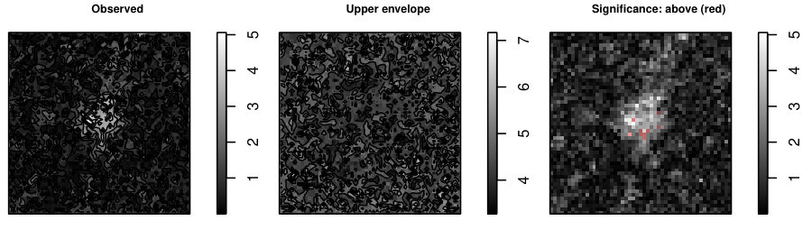 Figure 1
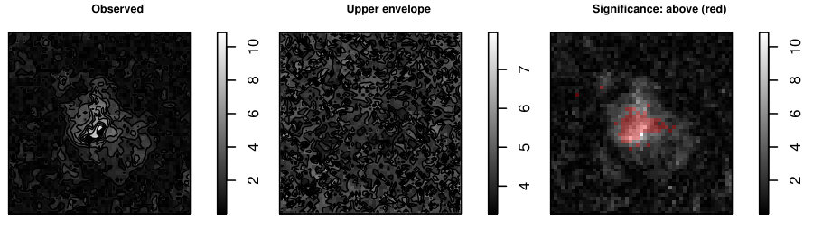 Figure 2
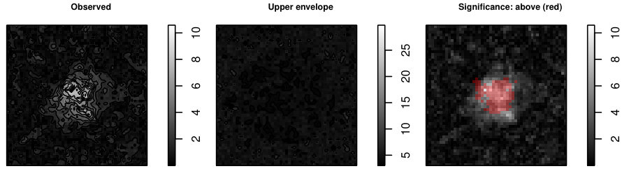 Figure 3
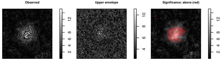 Figure 4
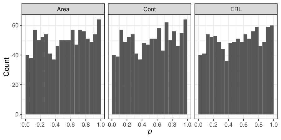 Figure 5
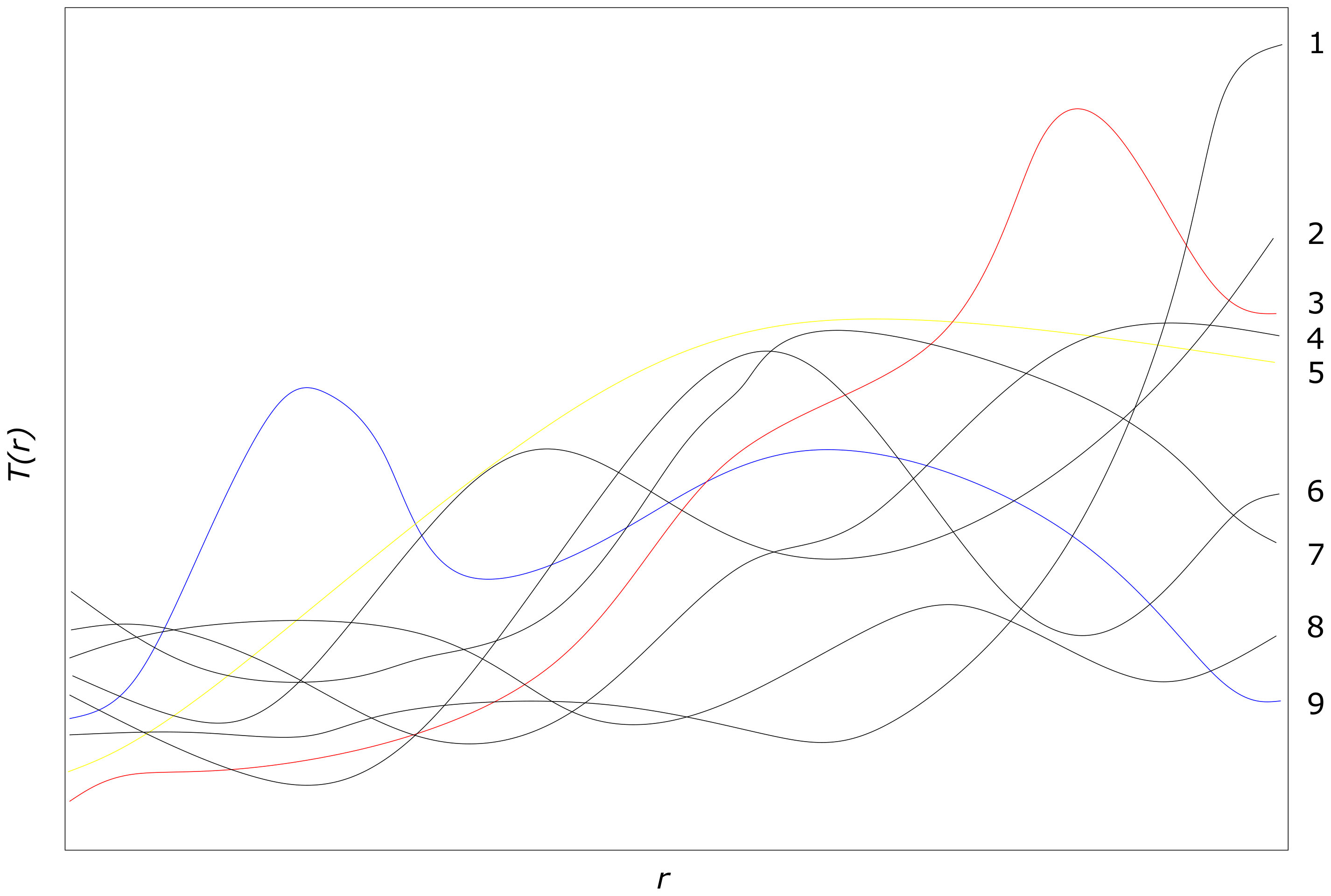 Figure 6
 Figure 7
 Figure 8
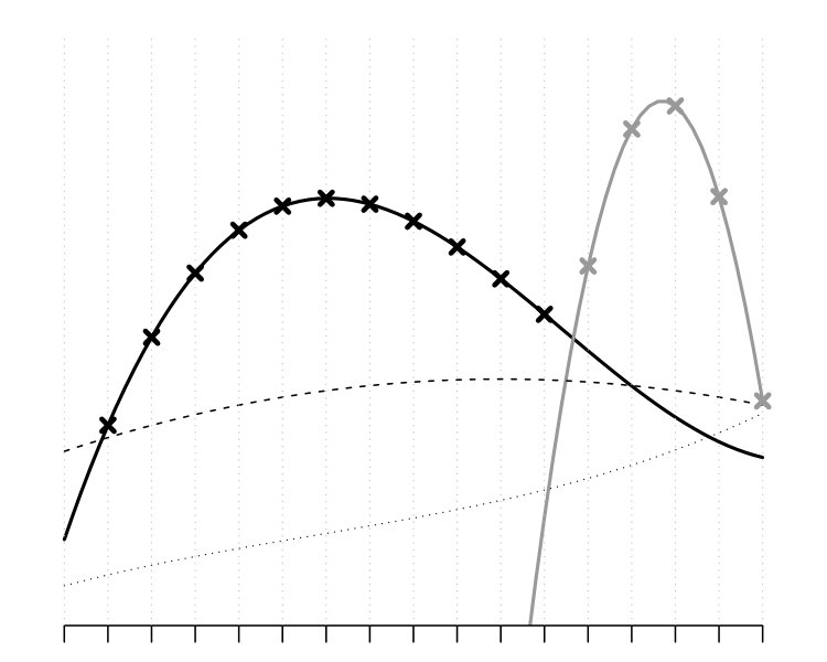 Figure 9
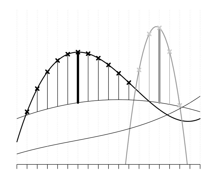 Figure 10
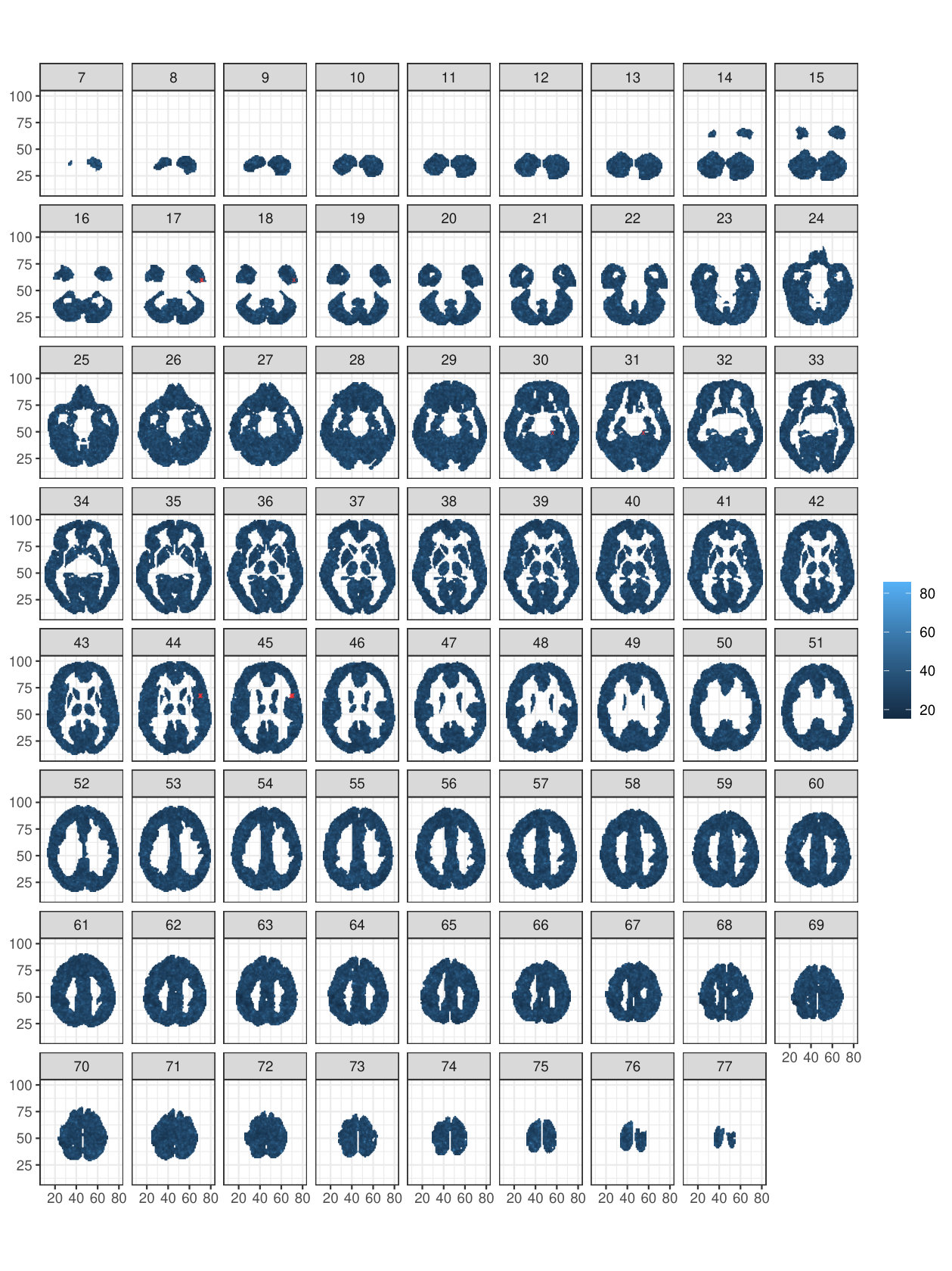 Figure 11
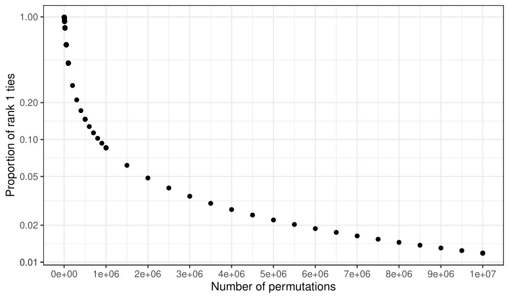 Figure 12
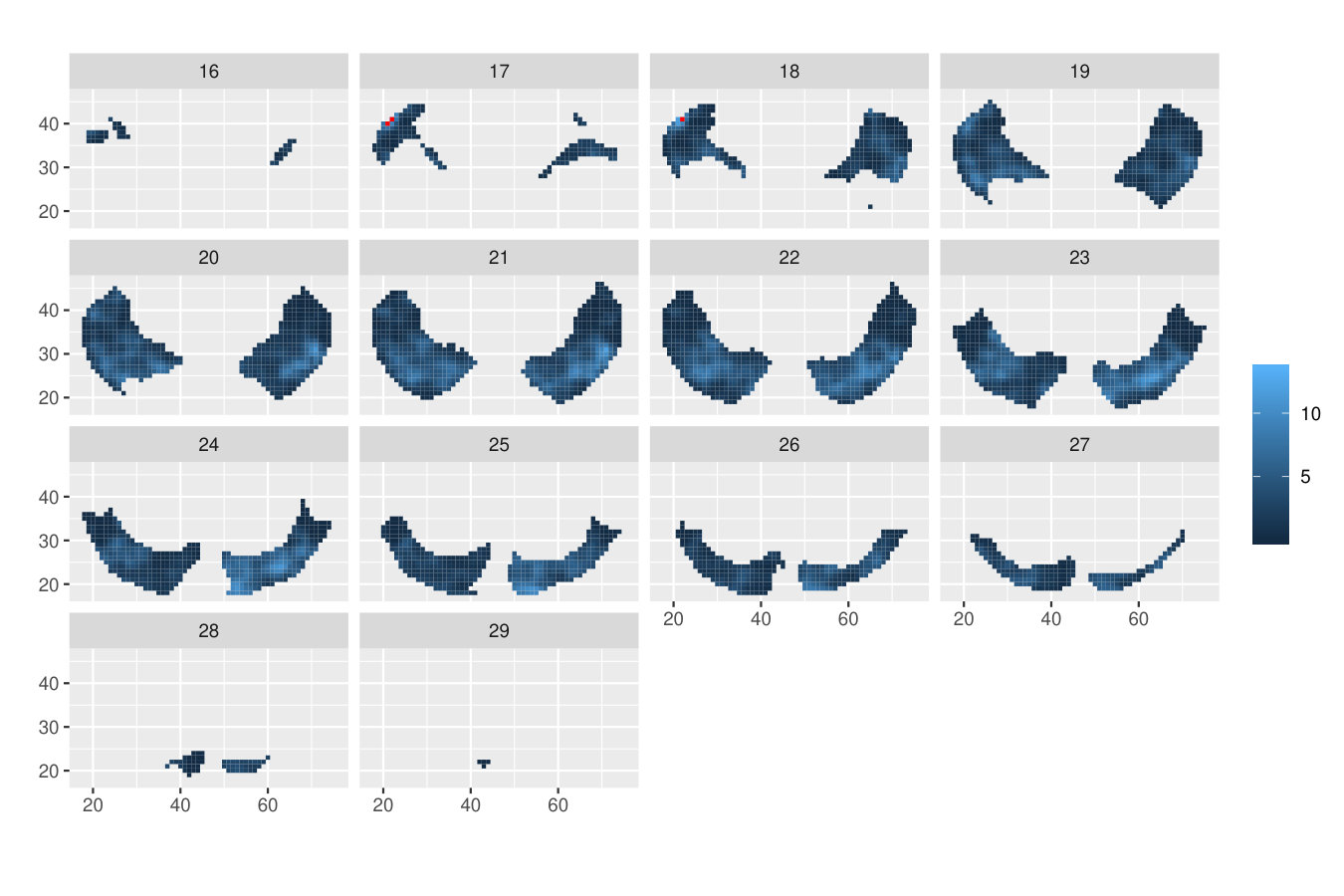 Figure 13
 Figure 14
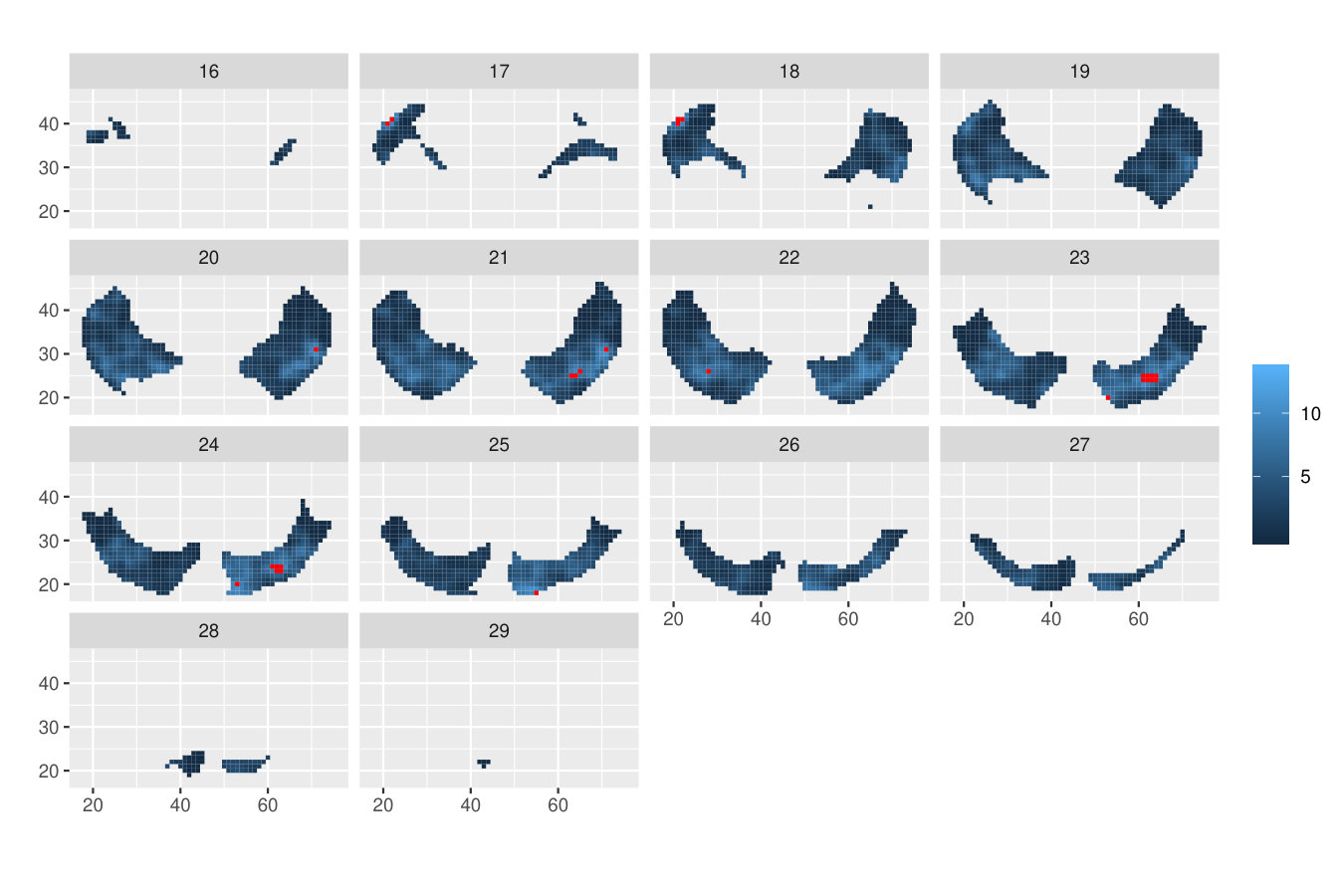 Figure 15
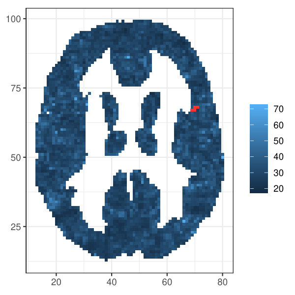 Figure 16
| Number of permutations | -max | -min | ERL | Cont | Area |
|---|---|---|---|---|---|
| 50000 | 0.058 | 0.592 | 0.032 | 0.105 | 0.040 |
| 100000 | 0.058 | 0.420 | 0.041 | 0.053 | 0.040 |
| Domain with | Value | ||
|---|---|---|---|
| -max | No | No | Yes |
| -min | Yes | No | No |
| ERL | Yes | Yes | No |
| Cont | Yes | No | Yes |
| Area | Yes | Yes | Yes |
| M0a- | M0b- | M0c- | M0d- | M0e- | M0f- | M0g- | |
|---|---|---|---|---|---|---|---|
| F-max | 0.054 | 0.056 | 0.040 | 0.046 | 0.053 | 0.058 | 0.043 |
| -min | 0.000 | 0.000 | 0.000 | 0.000 | 0.000 | 0.000 | 0.000 |
| ERL | 0.060 | 0.052 | 0.045 | 0.043 | 0.047 | 0.057 | 0.045 |
| Cont | 0.058 | 0.056 | 0.031 | 0.043 | 0.045 | 0.049 | 0.053 |
| Area | 0.058 | 0.047 | 0.040 | 0.040 | 0.043 | 0.061 | 0.045 |
| M1a- | M1b- | M1c- | M1d- | M1e- | M1f- | M1g- | |
|---|---|---|---|---|---|---|---|
| F-max | 0.395 | 0.464 | 0.267 | 0.334 | 0.294 | 0.632 | 0.421 |
| -min | 0.000 | 0.000 | 0.000 | 0.000 | 0.000 | 0.000 | 0.000 |
| ERL | 0.606 | 0.594 | 0.948 | 0.943 | 0.751 | 0.776 | 0.984 |
| Cont | 0.378 | 0.399 | 0.228 | 0.363 | 0.335 | 0.522 | 0.358 |
| Area | 0.544 | 0.568 | 0.879 | 0.909 | 0.577 | 0.749 | 0.979 |
| M1’a- | M1’b- | M1’c- | M1’d- | M1’e- | M1’f- | M1’g- | |
|---|---|---|---|---|---|---|---|
| F-max | 0.917 | 0.562 | 0.377 | 0.549 | 0.190 | 0.963 | 0.412 |
| -min | 0.000 | 0.000 | 0.000 | 0.000 | 0.000 | 0.000 | 0.000 |
| ERL | 0.732 | 0.365 | 0.972 | 0.752 | 0.235 | 0.720 | 0.894 |
| Cont | 0.799 | 0.461 | 0.339 | 0.445 | 0.221 | 0.899 | 0.408 |
| Area | 0.825 | 0.500 | 0.915 | 0.800 | 0.259 | 0.924 | 0.924 |
| Ties | Inhomogeneity and | Inhomogeneity of correlation | |
|---|---|---|---|
| non-normality of | structure of | ||
| -max | No | Yes | No |
| -min | Yes | No | No |
| ERL | No | No | Yes |
| Cont | No | Yes | No |
| Area | No | Partial | Partial |
| F-max | 0.054 | 0.048 | 0.043 | 0.051 | 0.044 | 0.045 | 0.047 |
| -min | 0.000 | 0.000 | 0.000 | 0.000 | 0.000 | 0.000 | 0.000 |
| ERL | 0.060 | 0.036 | 0.042 | 0.048 | 0.052 | 0.046 | 0.040 |
| Cont | 0.058 | 0.060 | 0.047 | 0.042 | 0.052 | 0.055 | 0.047 |
| Area | 0.058 | 0.040 | 0.041 | 0.053 | 0.047 | 0.050 | 0.040 |
| F-max | 1.000 | 1.000 | 1.000 | 0.863 | 0.395 | 0.184 | 0.106 |
| -min | 0.000 | 0.000 | 0.000 | 0.000 | 0.000 | 0.000 | 0.000 |
| ERL | 0.979 | 0.975 | 0.980 | 0.943 | 0.606 | 0.292 | 0.188 |
| Cont | 0.979 | 0.975 | 0.980 | 0.824 | 0.378 | 0.170 | 0.105 |
| Area | 0.979 | 0.975 | 0.980 | 0.929 | 0.544 | 0.257 | 0.150 |
| F-max | 1.000 | 1.000 | 1.000 | 0.886 | 0.464 | 0.242 | 0.151 |
| -min | 0.000 | 0.000 | 0.000 | 0.000 | 0.000 | 0.000 | 0.000 |
| ERL | 0.973 | 0.980 | 0.978 | 0.942 | 0.594 | 0.325 | 0.233 |
| Cont | 0.973 | 0.980 | 0.978 | 0.844 | 0.399 | 0.215 | 0.163 |
| Area | 0.973 | 0.980 | 0.978 | 0.927 | 0.568 | 0.303 | 0.215 |
| F-max | 1.000 | 1.000 | 0.959 | 0.267 | 0.097 | 0.067 | 0.058 |
| p-min | 0.000 | 0.000 | 0.000 | 0.000 | 0.000 | 0.000 | 0.000 |
| ERL | 0.986 | 0.976 | 0.979 | 0.948 | 0.520 | 0.269 | 0.175 |
| Cont | 0.986 | 0.976 | 0.945 | 0.228 | 0.090 | 0.065 | 0.050 |
| Area | 0.986 | 0.976 | 0.979 | 0.879 | 0.395 | 0.191 | 0.121 |
| F-max | 1.000 | 1.000 | 0.989 | 0.334 | 0.080 | 0.054 | 0.048 |
| p-min | 0.000 | 0.000 | 0.000 | 0.000 | 0.000 | 0.000 | 0.000 |
| ERL | 0.980 | 0.986 | 0.982 | 0.943 | 0.617 | 0.299 | 0.199 |
| Cont | 0.980 | 0.986 | 0.958 | 0.363 | 0.097 | 0.058 | 0.054 |
| Area | 0.980 | 0.986 | 0.982 | 0.909 | 0.492 | 0.229 | 0.157 |
| F-max | 1.000 | 0.997 | 0.979 | 0.857 | 0.609 | 0.410 | 0.294 |
| p-min | 0.000 | 0.000 | 0.000 | 0.000 | 0.000 | 0.000 | 0.000 |
| ERL | 0.980 | 0.970 | 0.977 | 0.967 | 0.930 | 0.844 | 0.751 |
| Cont | 0.980 | 0.968 | 0.960 | 0.865 | 0.662 | 0.491 | 0.335 |
| Area | 0.980 | 0.970 | 0.975 | 0.947 | 0.867 | 0.714 | 0.577 |
| F-max | 1.000 | 1.000 | 1.000 | 0.998 | 0.632 | 0.296 | 0.143 |
| -min | 0.000 | 0.000 | 0.000 | 0.000 | 0.000 | 0.000 | 0.000 |
| ERL | 0.981 | 0.980 | 0.985 | 0.985 | 0.776 | 0.325 | 0.126 |
| Cont | 0.981 | 0.980 | 0.985 | 0.971 | 0.522 | 0.249 | 0.129 |
| Area | 0.981 | 0.980 | 0.985 | 0.984 | 0.749 | 0.340 | 0.141 |
| F-max | 0.999 | 0.950 | 0.841 | 0.658 | 0.522 | 0.421 | 0.352 |
| -min | 0.000 | 0.000 | 0.000 | 0.000 | 0.000 | 0.000 | 0.000 |
| ERL | 0.986 | 0.980 | 0.977 | 0.979 | 0.981 | 0.984 | 0.978 |
| Cont | 0.985 | 0.917 | 0.790 | 0.604 | 0.448 | 0.358 | 0.300 |
| Area | 0.986 | 0.980 | 0.977 | 0.979 | 0.981 | 0.979 | 0.970 |
| F-max | 1.000 | 1.000 | 0.917 | 0.277 | 0.089 | 0.068 | 0.045 |
| -min | 0.000 | 0.000 | 0.000 | 0.000 | 0.000 | 0.000 | 0.000 |
| ERL | 0.975 | 0.976 | 0.732 | 0.201 | 0.071 | 0.064 | 0.052 |
| Cont | 0.975 | 0.975 | 0.799 | 0.230 | 0.077 | 0.058 | 0.048 |
| Area | 0.975 | 0.980 | 0.825 | 0.254 | 0.085 | 0.068 | 0.049 |
| F-max | 1.000 | 1.000 | 0.906 | 0.280 | 0.107 | 0.076 | 0.060 |
| -min | 0.000 | 0.000 | 0.000 | 0.000 | 0.000 | 0.000 | 0.000 |
| ERL | 0.980 | 0.962 | 0.705 | 0.193 | 0.076 | 0.071 | 0.053 |
| Cont | 0.980 | 0.962 | 0.811 | 0.232 | 0.099 | 0.068 | 0.070 |
| Area | 0.980 | 0.968 | 0.830 | 0.243 | 0.100 | 0.076 | 0.061 |
| F-max | 1.000 | 1.000 | 1.000 | 1.000 | 1.000 | 0.965 | 0.377 |
| p-min | 0.000 | 0.000 | 0.000 | 0.000 | 0.000 | 0.000 | 0.000 |
| ERL | 0.982 | 0.976 | 0.984 | 0.975 | 0.978 | 0.978 | 0.972 |
| Cont | 0.982 | 0.976 | 0.984 | 0.975 | 0.978 | 0.686 | 0.339 |
| Area | 0.982 | 0.976 | 0.984 | 0.975 | 0.978 | 0.978 | 0.915 |
| F-max | 1.000 | 0.993 | 0.549 | 0.060 | 0.066 | 0.062 | 0.048 |
| p-min | 0.000 | 0.000 | 0.000 | 0.000 | 0.000 | 0.000 | 0.000 |
| ERL | 0.979 | 0.973 | 0.752 | 0.188 | 0.097 | 0.074 | 0.056 |
| Cont | 0.979 | 0.907 | 0.445 | 0.080 | 0.053 | 0.054 | 0.047 |
| Area | 0.979 | 0.974 | 0.800 | 0.194 | 0.085 | 0.072 | 0.048 |
| F-max | 0.782 | 0.496 | 0.351 | 0.190 | 0.113 | 0.086 | 0.065 |
| p-min | 0.000 | 0.000 | 0.000 | 0.000 | 0.000 | 0.000 | 0.000 |
| ERL | 0.752 | 0.505 | 0.384 | 0.235 | 0.167 | 0.084 | 0.093 |
| Cont | 0.791 | 0.526 | 0.371 | 0.221 | 0.134 | 0.089 | 0.072 |
| Area | 0.826 | 0.583 | 0.422 | 0.259 | 0.163 | 0.093 | 0.087 |
| F-max | 1.000 | 1.000 | 0.963 | 0.358 | 0.089 | 0.058 | 0.057 |
| -min | 0.000 | 0.000 | 0.000 | 0.000 | 0.000 | 0.000 | 0.000 |
| ERL | 0.975 | 0.978 | 0.720 | 0.110 | 0.059 | 0.051 | 0.045 |
| Cont | 0.975 | 0.979 | 0.899 | 0.275 | 0.083 | 0.062 | 0.047 |
| Area | 0.975 | 0.979 | 0.924 | 0.258 | 0.077 | 0.056 | 0.048 |
| F-max | 0.412 | 0.228 | 0.146 | 0.101 | 0.084 | 0.073 | 0.067 |
| -min | 0.000 | 0.000 | 0.000 | 0.000 | 0.000 | 0.000 | 0.000 |
| ERL | 0.894 | 0.589 | 0.311 | 0.193 | 0.186 | 0.132 | 0.120 |
| Cont | 0.408 | 0.189 | 0.124 | 0.094 | 0.081 | 0.063 | 0.073 |
| Area | 0.924 | 0.612 | 0.424 | 0.292 | 0.208 | 0.154 | 0.134 |
Peer Reviews
No public reviews on file for this paper yet. If you reviewed it on a platform where reviews are public (OpenReview, ICLR, NeurIPS, ICML), you can paste yours below so the community can read it here.
Videos
No videos yet. Explain this paper in a talk, walkthrough, or lecture? Add one.
New methods for multiple testing in permutation inference for the general linear model
Tomáš Mrkvička1,2
Faculty of Economics, University of South Bohemia, Czech Republic
Mari Myllymäki
Natural Resources Institute Finland (Luke), Helsinki, Finland
Mikko Kuronen
Natural Resources Institute Finland (Luke), Helsinki, Finland
Naveen Naidu Narisetty
University of Illinois, Urbana-Champaign, USA
Abstract
Permutation methods are commonly used to test significance of regressors of interest in general linear models (GLMs) for functional (image) data sets, in particular for neuroimaging applications as they rely on mild assumptions. Permutation inference for GLMs typically consists of three parts: choosing a relevant test statistic, computing pointwise permutation tests and applying a multiple testing correction. We propose new multiple testing methods as an alternative to the commonly used maximum value of test statistics across the image. The new methods improve power and robustness against inhomogeneity of the test statistic across its domain. The methods rely on sorting the permuted functional test statistics based on pointwise rank measures; still they can be implemented even for large brain data. The performance of the methods is demonstrated through a designed simulation experiment, and an example of brain imaging data. We developed the R package GET which can be used for computation of the proposed procedures.
keywords:
Function-on-scalar regression, General linear model , Global envelope test , Graphical method , Multiple testing correction , Permutation inference
myfootnotemyfootnotefootnotetext: Corresponding author: [email protected]: Dpt. of Applied Mathematics and Informatics, Faculty of Economics, University of South Bohemia, Studentská 13, 37005 České Budějovice, Czech Republic
1 Introduction
General linear models (GLMs) are among the most commonly used statistical tools in the field of neuroimaging for analyzing imaging data [Christensen, 2002]. To perform statistical inference based on GLMs, one approach is to use parametric methods which rely on stringent assumptions, such as the normality of the random errors in the GLM, homogeneity and independence of the random errors across the image. Alternatively, one can use non-parametric methods with weaker assumptions about the data [see e.g. Winkler et al., 2014, Table 1].
Permutation tests are a class of non-parametric methods, which have a long history going back to Fisher [1935]. Fisher demonstrated that the null hypothesis could be tested by observing, how often the test statistic computed from permuted observations would be more extreme than the same statistic computed without permutation. Even though the data in neuroimaging applications are commonly images, the same principle still holds; a detailed introduction to the permutation inference for the GLMs for neuroimage data can be found in Winkler et al. [2014]. Another advantage of the non-parametric methods is that they do not suffer from the false positive rates reported by Eklund et al. [2016] for parametric approaches.
Analysis based on permutation tests consists of several crucial steps. First, a suitable test statistic that is computed for each single location (spatial point, voxel, vertex or face) of an image has to be chosen such that it is informative about the studied null and alternative hypotheses and homogeneous across the image. Second, the appropriate permutation scheme has to be used to generate the permutations from the studied null hypothesis. The permutations are performed between subjects, thus throughout the whole paper we discuss the second-level analysis. Finally, an appropriate multiple testing correction has to be applied to significance results obtained for all spatial locations by the permutation test.
Commonly used test statistics include the - and -statistics, or the statistic defined in Winkler et al. [2014] which generalises the classical statistics into various cases with heteroscedasticity. However, a serious limitation of the or statistics is that they are not pivotal across different locations of the image in terms of the entire distribution, but only in terms of the first and second moments when the errors are not normally distributed. Therefore, if the error distribution is non-normal and inhomogeneous across the image, the distribution of these test statistics varies across the image causing the desired quantiles of the test statistics to vary as well. For example, if the error term has lognormal distribution with parameters 1 and 2 on one side of the image and with parameters 1 and 0.5 on another part of the image, then the ratio of 95% quantiles of the -statistic computed from 20 observations is equal to 1.37. The ratio of 99% quantiles is 1.64. (These ratios were computed from simulated sample of 10000 -statistics under the null hypothesis.) If this heterogeneity is ignored, e.g. by taking the maximum -statistic across the spatial points as the test statistic, some or all spatial points where the null model is broken may be overlooked. In quantitative manner, this can bring a substantial loss of power as we demonstrate in our simulation study.
Due to the non-pivotal nature of the and statistics, a more suitable choice is the permutation -value, which is automatically a pivotal statistic, i.e. its distribution does not change across the image. Therefore, it would be convenient to perform the multiple testing correction by taking the minimum -value across the image as the test statistic. However, the permutation -value has another serious disadvantage: due to its discreteness, the (minimum) -values obtained from permutations contain ties and the resulting test tends to be conservative, leading to loss of power as well [Pantazis et al., 2005]. This disadvantage is enormous especially in the case of high resolution images where the number of permutations can not be large due to computational limitations. This is further demonstrated in the introductory example below.
Another problem arises for test statistics which accumulate the data from the surrounding area of a single spatial location, e.g. the local area above a given threshold around a spatial location. Namely, if the spatial autocorrelation of the data is inhomogeneous across the image, then the sizes of the areas above the thresholds in different parts of the image are not comparable. This problem was recently treated for the special case of cluster size permutation tests in Hayasaka et al. [2004] and Salimi-Khorshidi et al. [2011]. In this paper we discuss solutions for the case of inhomogeneous spatial autocorrelation and also for the case of inhomogeneous distribution of the test statistic.
The classical multiple testing procedures, computing the maximum (-max) or the minimum -value (-min) statistic across all spatial points, control the family wise error rate (FWER) [see e.g. Winkler et al., 2014]. This paper introduces three new multiple testing corrections for the permutation inference for the GLMs, controlling the FWER in a similar manner.
The new methods are alternative solutions to the ties problem of -values. The first correction is based on the extreme rank length (ERL) measure that was originally proposed by Myllymäki et al. [2017] and Narisetty and Nair [2016] for spatial and functional data analysis. The other two corrections rely on the continuous rank measure (Cont) introduced in the technical report of Hahn [2015] and the area rank measure (Area) presented in this work first time. We carefully describe the homogeneity assumptions of the -max, -min and new methods and further their sensitivity to different types of extremeness of the test statistic. By a simulation study, we illustrate the power of the new and existing tests under different scenarios, both when the homogeneity assumptions of the multiple correction methods are met and when not. A further asset of the methods, namely a graphical interpretation of the test results in a similar manner as in global envelope testing [Myllymäki et al., 2017, Mrkvička et al., 2016, 2018], is illustrated by a real data example of autism brain imaging data [Di Martino et al., 2014]. We conclude that the choice of the measure for multiple correction should be done on the basis of reasonable assumptions of different types of homogeneity, and the expected type of extremeness of the test statistic.
The proposed tests are implemented in the R library GET [Myllymäki et al., 2017, Myllymäki and Mrkvička, 2020].
1.1 Introductory example
To illustrate the proposed methods, we studied the autism brain imaging data collected by resting state functional magnetic resonance imaging (R-fMRI) [Di Martino et al., 2014]. The raw fMRI data contains measurements from 539 individuals with the autism spectrum disorder (ASD) and 573 typical controls (TC). When the number of individuals in the analysis is large, the test statistics can be well approximated by the limiting distribution. Therefore, in order to show the differences between the methods, we have chosen a small number of individuals, namely the patients measured in Oregon Health and Science University with 13 subjects with Autism Spectrum Disorders (ASD), 15 Typical Controls (TC) and homogeneity in sex. In fact, when the whole dataset of 1112 patients was used in our analysis, the -max procedure worked equally to our proposed methods. The imaging measurement for local brain activity at resting state was fractional amplitude of low frequency fluctuations [Zou et al., 2008]. The whole brain was analyzed consisting of 175 493 voxels. The difference between the groups was studied while age was taken as a nuisance factor. The -max, -min and new tests were performed using the same 50 000 and 100 000 permutations. The experiment was run using the R package GET [Myllymäki and Mrkvička, 2020] and took 10 hours using two cores and 10 Gb memory of an ordinary laptop. Most of this time was allocated to calculating the -statistics for each permutation and each voxel, which were needed for all tests.
Table 1 shows the -values of all the investigated methods. While the differences in the -values are small between the -max and new methods, only the ERL and Area tests rejected the null hypothesis of no group effect at the strict significance level 0.05. An essential difference between the -max and new methods is in their critical bounds: Figure 1 shows the 95% global upper envelope of the global Area test for one slice of the brain; Appendix B presents the results for the whole brain. This upper envelope is adjusted to the variability of the 95% global quantile of the -statistics, ranging from 20 to 70 for the given slice. If the empirical -statistic crosses the 95% global quantile, the null hypothesis is rejected. On the other hand, the critical bound of the -max test is constant (48.4), therefore the -max procedure can overlook significant voxels where the variability of the -statistics is smaller.
The -min procedure, which is also adjusted to the variability of the statistics across the image, was highly conservative for 50 000 or 100 000 permutations (Table 1). Figure 2 further shows the proportion of permutations which achieved the most extreme -statistic at least for one voxel for different numbers of permutations. This value corresponds to the minimal -value that the -min procedure can achieve. This example with the total of 10 000 000 permutations was run on a computing server with hundreds of cores. Thus if one needs the -min procedure to give an answer for the test of the whole brain, 6 000 000 of permutations has to be used in minimum to achieve the minimal -value 0.02 (which is still not very precise procedure), and this is typically too much.
The aim of this paper is to give three solutions for breaking the ties of the -min procedure which can be used with reasonable number of permutations, i.e. in the time comparable to the time required by the -max procedure. The proposed methods also provide the correct significance level as it is shown by simulation study in Section 3 and also by an experiment similar to one proposed in Eklund et al. [2016], which we report in Appendix A.
2 Multiple testing correction for permutation methods
Let us consider the GLM
[TABLE]
where the argument determines a spatial point of the image or, generally, a location where the -dimensional functions, , are observed. The number of locations will be denoted by . For every location , we consider a one-dimensional GLM with being a matrix of regressors of interest, being a matrix of nuisance regressors, being a vector of observed data and being a vector of random errors with mean zero and finite variance for every . Further assumptions about the error structure will be given along the definitions of the multiple correction methods below. Further, and are the regression coefficient vectors of dimensions and , respectively. Often factors are given for the whole image, as in our examples as well. In this case the regressors do not depend on the index and so the matrices and are identical for every . However, this simplification is not necessary. The null hypothesis to be tested is
[TABLE]
where is a matrix of contrasts of interest.
The GLM setup includes a wide range of applications in neuroimaging, see Winkler et al. [2014] for worked examples. Under various setups, a nonparametric pointwise permutation test can be applied to obtain a set of -values, . We refer to the detailed description of pointwise permutation tests in Winkler et al. [2014]. Shortly, first a test statistic is chosen from a vast number of possibilities, reflecting the tested null model and heteroscedasticity. A common choice is the -statistic [Christensen, 2002], but in principle any statistic where extreme values reflect evidence against the null hypothesis could be used. Then permutations are used to obtain the distribution of under the null hypothesis . The choice of the permutation scheme is important for the performance of the method. We chose the permutation of the residuals under the null model [Freedman and Lane, 1983], which is approximate, but according to Anderson and Ter Braak [2003] it is the most precise permutation method in the case of nuisance effects [see also Winkler et al., 2014]. If there are no nuisance regressors, except the constant, permutation of raw data can be used instead; it is however equivalent to performing the Freedman-Lane algorithm since the fit of the null model is constant in this case. In this case, the test is exact. The last step is to apply a multiple testing correction.
Following sections describe various multiple testing corrections in these permutation procedures. We assume that the same permutations have been applied for every location . We denote the test statistic calculated for the original data by and the corresponding test statistics calculated for each permutation , , by . Further, , , denotes the set of pointwise -values for the test statistic of the original data, and by the corresponding -values for each permutation , .
2.1 The -min approach
In the -min approach, the minimum of the pointwise -values,
[TABLE]
are calculated for all , and the Monte Carlo -value is obtained as
[TABLE]
Here denotes the indicator function.
The pointwise -values are pivotal, therefore the -min approach needs no further assumptions about the random error . However, since the -values of the permutation test can achieve only values , many ties can appear among , especially for large , leading to a conservative test.
2.2 Refinements of the -min approach
The -min approach is in fact equivalent to the global rank envelope test defined by Myllymäki et al. [2017] for spatial processes. I.e., the is after a simple normalization equivalent to the extreme rank measure :
[TABLE]
where is the pointwise rank of the test statistic among such that the smallest value obtains the rank 1. The measures and the corresponding global envelopes are defined here as one-sided since the extremeness of the test statistic used in the GLM is usually realized only for high values. This one-sided alternative also leads to in the right hand side of the formula (3).
In the sequel, we propose the following three methods for breaking the ties between the values:
The extreme rank length (ERL) approach takes into account the number of pointwise -values equalling the minimal -value ,
- 2.
the continuous rank (Cont) approach measures the maximal size of extremeness of that is associated with , and
- 3.
the area rank (Area) accumulates the extremeness of across the spatial points where is obtained.
2.2.1 Extreme rank length (ERL)
The ERL measure refines the -min approach in the sense that not only the minimal -value , but also the size of the domain where are equal to is taken into account. Typically, based on our experience, the ties are already broken by considering the counts of the smallest pointwise -values among . However, to define the ERL measure [Myllymäki et al., 2017, Narisetty and Nair, 2016, Mrkvička et al., 2018] formally, the complete vectors of pointwise ordered -values , where the pointwise -values observed at are arranged from smallest to largest such that whenever , are considered and ordered by reverse lexical ordering: The ERL measure is equal to
[TABLE]
where
[TABLE]
and scales the values to the interval from 0 to 1. Thus, the ERL measure uses in fact all the pointwise -values to order the test statistics from most extreme to the least extreme one, while the -min procedure utilizes only .
Since the probability of having a tie in the ERL measure is rather small, the application of Monte Carlo test on the ERL solves the ties problem [see also Myllymäki et al., 2017]. Thus the final -value is .
Because often even the counts of the most extreme -values break the ties, the measure can be efficiently implemented utilizing the counts of a certain number (e.g. six) of smallest pointwise -values (see Section 4).
2.2.2 Continuous rank (Cont)
Another refinement of is the continuous rank measure
[TABLE]
where is the continuous pointwise rank that is a refinement of the ordinary rank based on the relative magnitude of the test statistic with respect to the other , . The continuous rank is defined such that the smallest value of obtains the smallest continuous rank: Let denote the ordered set of values . Then the continuous rank of is
[TABLE]
and
[TABLE]
If the probability to have ties among , is zero, then the probability of ties among is zero as well. If ties appear among , i.e. , then the continuous rank is defined as for . The continuous ranks were first suggested by Hahn [2015], and are defined here with a slight modification in the scaling of and .
Finally, the univariate Monte Carlo test is performed based on . Thus the final -value is .
2.2.3 Area rank
The last refinement is the area rank measure defined as:
[TABLE]
where is equal to the number of . Thus, the area measure refines the extreme rank by reducing from it the scaled sum of the differences between and across the spatial points where the minimal -values (or ranks) are obtained. Thus, the larger the amount of those critical and the smaller the pointwise continuous ranks at those critical are, the smaller is the value of the area measure, i.e. the more extreme the corresponding test statistic . The univariate Monte Carlo test is performed based on with .
2.3 Illustration of the new measures
Figure 3 shows a small set of one-dimensional functions (test statistics) for description of the behaviour of the new measures. Only large values of are considered significant. In this set of functions, the variance of the distribution of increases along (from left to right). According to the -max method the most extreme test statistic is the function 1 reaching the overall highest value across the locations . On the other hand, the -min method gives the minimal -value to six functions (1, 3, 4, 5, 7 and 9). The refinement measures decide the extremeness of these functions by different rules.
The most extreme function according to the ERL measure is the function 5 (yellow), because it obtains the largest value, i.e. the minimal -value, over the largest domain. On the other hand, according to the continuous and area rank measures, the most extreme function is the function 9 (blue): The deviation of the functions 3 (red) and 9 (blue) from the second most extreme functions is of the same size at those locations where these functions reach the minimal -value. However, the scaling of the continuous rank by the overall variation (see Eq. (6)) leads to smaller pointwise continuous ranks for the function 9, therefore also to a smaller overall continuous rank. Because the two functions reach the minimal -values approximately at domains of the same size, also the area measure deduces the function 9 as the most extreme function.
This example illustrated two issues:
- The fact that the ERL, continuous and area measures are all refinements of the -min method allows them to regard as most extreme also functions which reach their minimal -value, , at locations where the variation of the functions is small.
- The refinement measures break the ties by different rules as summarized in Table 2.
2.3.1 Graphical interpretation - % global envelope
Consider any of the three measures we defined and denote them using a common notation . Let be the index set of the test statistics, where the threshold is chosen to be the largest value in for which
[TABLE]
i.e. the set contains the indices of the % of the least extreme test statistics . The global envelope is defined to be
[TABLE]
As a consequence, the probability that falls outside this global envelope in any of the points is less or equal to ,
[TABLE]
The following theorem states that inference based on the -value (where stands for and ) and on the global envelope specified by and with respect to the appropriate measure are equivalent. Therefore, we can refer to these envelopes as the % global extreme rank length envelope, continuous rank envelope and area rank envelope. Figure 1 shows an example of the extreme rank length upper envelope together with red points indicating the area where the test function crossed this envelope. Thus the graphical interpretation identifies the voxels which cause the rejection.
Theorem 2.1**.**
Assume that there are no pointwise ties with probability among . Then
* for some iff , in which case the null hypothesis is rejected;* 2. 2.
* for all iff , and thus the null hypothesis is not rejected;*
Proof.
Since 1. holds iff 2. holds, it’s enough to show 1. According to the definition of , iff number of smaller or equal to is smaller or equal to . That is equivalent, according to the definition of to . This holds iff , which is equivalent to for some according to the definition of the measure .
∎
2.4 -max approach
Usually the statistic is one of the statistics used in the parametric general linear models, i.e. -statistic, -statistic, or variance weighted -statistic. In these cases, an immediate solution to the problem of ties is to replace statistic in the Monte Carlo test directly by the statistic, but with the price of loosing the pivotality and, consequently also the power. See the next section for details.
3 Simulation experiment
To compare the power and robustness of the proposed methods and the existing multiple comparison methods under different scenarios, we generated synthetic imaging data mimicking real data from neuroimaging studies. We considered a categorical factor taking the values 1 or 2 according the group to which the image belongs to, and a continuous factor that was generated from the uniform distribution on . We simulated images in the square window on a grid of pixel resolution from the following GLM models:
[TABLE]
[TABLE]
and
[TABLE]
The image resolution is obviously small in comparison the brain data (see Section 1.1), but was regarded as sufficient for the designed experiment to show differences between the measures. Here denotes the Euclidean distance of the pixel to the origin and is a zero-mean correlated error. The model M0 has no factors and generates purely noisy images, the models M1 and M1’ generate two groups of images depending on the categorical factor and the model M2 generates images which depend on both the categorical and continuous factors. The models M1 and M1’ correspond to simple comparison of two groups of images, where the ”bump” at the center of the image is two times higher for second group than for the first group. The area where the two groups differ is about hundred times smaller in the model M1’ than in M1. Because in M1 the departures from the null model occur for many pixels and the ERL and Area methods accumulate information across the pixels, the ERL and Area methods are expected to have advantage over the other methods in this model. On the other hand, the departures from the null model are expected only for a few pixels in M1’ and, thus, such advantage does not occur in this model.
The model M0 is a null model where the images in the two groups are from the same model (no factors) and it was used for estimating the significance levels of the different tests. The model M2 is similar to M1, but the groups are disturbed by the continuous factor . The models M1, M1’ and M2 were used for power estimation. The permutation of raw data was used in models M1 and M1’. The Freedman and Lane permutation scheme was used in M2. Because the model M2 revealed consistent results with model M1, the results are not presented.
For both models M1 and M1’, seven different correlated error structures were considered:
- (a)
Gaussian error , where is a Gaussian random field with the exponential correlation structure with scale parameter and standard deviation which will take several values,
- (b)
skewed error ,
- (c)
shape inhomogeneous distribution with increasing bimodality
,
- (d)
, i.e. inhomogeneous distribution over with the bimodal and normal errors in the periphery and in the middle of the image, respectively,
- (e)
, i.e. inhomogeneous distribution over with the skewed and normal errors in the middle and periphery of the image, respectively,
- (f)
, i.e. Gaussian distribution with inhomogeneity in the correlation structure (scale parameters 0.05 and 0.3 in the middle and periphery of the image),
- (g)
, i.e. bimodal distribution with inhomogeneity in the correlation structure.
The homogeneous error distributions (a) and (b) represent cases where all methods should perform well in identifying alternative hypothesis. The skewed error (b) represents a situation where the permutation inference is necessary because the assumptions needed for parametric methods are not met. Further, the errors (c), (d) and (e) are inhomogeneous across the image and illustrate cases where the variability of the test statistic in the periphery of the image mask the signal from the center of the image. The error (c) is rather normal in the center of the image while the increasing bimodality appears closer to the periphery. The bimodal error corresponds to the sharp changes in the images, whereas Gaussian error corresponds to the smooth changes in the images. The errors (d) and (e) have normal error at different places, in order to have bigger quantiles of the test statistic at the periphery of the image. On the other hand, the errors (f) and (g) are used to investigate the effect of inhomogeneity in the correlation structure on the results.
All the images in the simulation study had the resolution pixels. The number of permutations used throughout the whole simulation study was set to 2000. The estimated significance levels and powers were recorded for various cases for all studied multiple comparison methods, i.e. for -max, -min and the proposed ERL, continuous and area rank methods.
To capture the behavior of the methods for various levels of significance, seven different standard deviations , , , , , and were used in all studied cases. Each model was simulated with ten images per group and each experiment was repeated 1000 times in order to obtain estimated significance levels and powers.
Tables 3, 4 and 5 show the results for models M0, M1 and M1’ in a shorted way. The detailed results are presented in Appendix C.
The estimated significance levels revealed the same structure for all errors (a)-(g) (Table 3): The -min was enourmously conservative. The -max and all our proposed methods achieved the preset significance level in all cases. (The 95% confidence interval for 1000 simulations with success probability 0.05 is (0.037, 0.063).) The only exception was the error (c), where Cont was slightly conservative.
The conservative -min method had no power (Tables 4 and 5). The ERL and Area methods had uniformly higher power than -max for all errors in case of the model M1. This is caused by the fact that ERL and Area summarize the extremeness of the test statistic from all spatial points. This advantage led to higher power even in the cases (f)-(g) with inhomogeneous autocorrelation.
The situation is more complicated for model M1’, where the area of extremeness is rather small: the ERL and Area can not benefit from their feature of collecting information from all spatial points. For the homogeneous cases with normal error (a) and skewed error (b), the -max is slightly more powerful than our proposed methods. When the inhomogeneity of errors is set in such a way that the values of the test statistic quantiles are larger at periphery where no differences are present – cases (c), (d) and (e) – the ERL and Area methods are significantly more powerful than -max (Table 5). Finally, when the range of correlation is larger at the periphery where no differences are present, the methods accumulating information from neighborhood should be affected by this fact. Really, in case (f) ERL appears to be less powerful than -max, but the Area method which uses different sources of information (see Table 2) is affected by this fact only little. This decrease of power is not further seen in case (g) where the normal distribution is replaced by the bimodal distribution. At last, we observe that Cont and -max methods were rather equivalent in our study with 2601 spatial points and 2000 permutations.
4 Computational details: how to implement the methods for large brain data
The -min, ERL, Cont and Area measures are based either on ordinary or continuous pointwise ranks of the test statistics , , among each other. A naive algorithm would first calculate all the ranks and save them in the memory in order to calculate the measures thereafter. However, the space complexity of the naive algorithm is , and for large data all the ranks may not fit comfortably to the memory of an ordinary computer. However, for all the proposed measures, it is possible to split the task by the locations (voxels) . In this case, the space complexity is just , where is the number of subjects. We note that the space complexity can be even further reduced to if the permutations are not saved. This can be achieved by resetting the seed of the pseudo random number generator for each split. This is typically not necessary.
There is some extra computational complexity of the rank based multiple comparison in comparison to the -max method because the test statistics need to be ranked. Namely, letting denote the time complexity of the test statistic to be computed, the complexity of computing rank based multiple comparison correction is , while for -max it is . Thus, asymptotically the rank based corrections are slower than -max. This is the same whether the naive or location-wise calculations are used.
Algorithm 1 presents the algorithm for location-wise (voxel by voxel) calculation of the rank-based measures. The update rules and calculation of the final measures are described thereafter for the different measures in Sections 4.1, 4.2 and 4.3. The implementation is obvious for the -min and Cont measures, while for ERL and Area, some more complicated calculations are needed. The computations are implemented in the function partial_forder of the R package GET [Myllymäki and Mrkvička, 2020]. Section 4.4 explains how the global envelope can be calculated given the measures.
4.1 Update rule for -min and Cont
For the -min and Cont measures, the update rule is simple:
[TABLE]
When all locations have been handled, the final measure, either or , is obtained by dividing the by .
4.2 Update rule for Area
For the Area and ERL measures, it is necessary to augment the measure with some auxiliary information during the computation. Namely, for the Area measure, the extreme rank and the difference between the extreme rank and the pointwise continuous rank has to be saved and updated for data and each permutation . Let denote the difference. Initially . For the update there are three possibilities:
[TABLE]
The final measure is
[TABLE]
4.3 Update rules for ERL
For ERL, the augmented measure is a vector of the chosen number of most extreme pointwise ranks of and their counts among . We record the six most extreme ranks, thus let
[TABLE]
be the initilized vector. Then the updates are obtained by the following rules:
If for some , then .
- 2.
If for some , then
[TABLE]
and .
The final measure for ERL is the ranking of the augmented measures according to a special ordering that is defined as follows. Let and be the augmented measures for two functions 1 and 2.
Start with the most extreme rank 2. 2.
if then function 1 is more extreme. 3. 3.
if then function 2 is more extreme. 4. 4.
if and then function 2 is more extreme. 5. 5.
if and then function 1 is more extreme. 6. 6.
if and then set and go to step 2.
The final normalized ERL measures (4) are obtained by dividing by .
4.4 Computation of the global envelopes
After the final measures have been calculated and the -value of the test is less than the chosen significance level, it is possible to construct the envelope to detect which parts of the domain have led to the rejection of the null hypothesis. Algorithm 2 describes the computation.
5 Discussion
All the permutation based multiple testing procedures reach the prescribed significance level, if the permutation strategy leads to exchangeable test statistics. They even reach the prescribed level approximately in the presence of nuisance factors, if the Freedman and Lane permutation strategy is used. This fact was demonstrated here by a simulation study and the Eklund et al. [2016] type of experiment presented in Appendix A.
The measures used in the permutation test are different in two ways, their sensitiveness towards different types of extremeness and their robustness against different types of inhomogeneities of the error term across . The sensitivities can be understood from the sources of information which are gathered by the different measures (see Table 2): The integral type of extremeness is detected by those measures (ERL, Area) that gather information across the locations with the minimal -values, while the measures based on the value of extremes (Cont, Area) are sensitive to maximum type of extremeness. The categorization is given by the construction of the measures, and it was further supported by the simulation study results for cases M1 and M1’.
Table 6 summarizes the investigated measures and their problems with identification of the alternative hypothesis, i.e. with ties and various inhomogeneities of the error term. The inhomogeneities can decrease the power of the procedures as stated in the table. As it was stated already in the introduction, the inhomogeneity and non normality of error term across together lead to inhomogeneous quantiles of the -statistic. Therefore, the -max procedure can be blind to the departures where the quantiles of are less variable. This was demonstrated in Section 1.1 and in the simulation study by cases c), d) and e). Since the Cont measure depends also on the values of and not only ranks, the Cont measure has the same problem as -max with inhomogeneity of . However, the problem of Cont depends on the number of ties to break: the bigger their number is, the less sensitive Cont is expected to be to inhomogeneity.
On the other hand, in the presence of the inhomogeneity of the correlation structure of across , the ERL measure can be blind to the departures from the null that occur in areas where the range of correlation of is smaller. This was demonstrated by the simulation study cases f) and g).
The Area rank measure is a combination of Cont and ERL, and thus it should be sensitive to both inhomogeneities but as the simulation study shows the decrease of power in cases c), d), e), f) and g) was not as apparent as for the -max, ERL or Cont procedures. Thus the Area measure appears to be the most robust method with respect to inhomogeneity of the error term .
Further, the simulation study case g) showed that the rank based measures are much more robust with respect to extreme non normality than the -max test as the decrease of power between cases f) and g) is apparent only for -max procedure.
6 Conclusions
We presented three new multiple comparison methods for the permutation inference for the GLM. We showed by a designed experiment that the proposed methods have the desired significance level unlike the -min method that was highly conservative, unless enormous amount of permutations was used. The choice of the method from -max, ERL, Cont and Area rank measures should depend on the assumptions about error term that can be made and the expected type of extremeness of the test statistic. Both homogeneity of the distribution of (HD) and homogeneity of the correlation structure of (HCS) across the image play a role (see Table 6). When we assume
both HD and HCS, then all methods can be applied. The ERL or Area methods should be preferred when the test statistic is expected to be extreme over a large area of the image ; -max, Cont or Area when extremeness is expected only on a small area. The same recommendations hold, if the assumption of homogeneity of is replaced by the assumption of the normality of the error .
- 2.
HCS but not HD, then only ERL can be applied without worry of loosing power to identify alternative hypotheses. However, in our designed experiment, Area showed good robustness with respect to inhomogeneity of the distribution of , whereas -max and Cont did not.
- 3.
HD but not HCS, then -max and Cont can be applied without worry of loosing power to identify alternative hypotheses. Again Area showed good robustness with respect to inhomogeneity of the correlation structure of , whereas ERL did not.
- 4.
neither HD nor HCS, then none of the methods can be applied without worry of loosing power to identify alternative hypotheses, but Area showed good robustness with respect to both types of inhomogeneities.
Thus, our experience suggests that the Area method can be used in a general situation without worry of loosing much power. Its dual nature of being based both on extremeness of the test statistic as well as on summarizing this extremeness across spatial points makes it sensitive to different departures from the null model and robust to different kinds of inhomogeneity. This was demonstrated by a designed experiment as well as an example of a real data study, where the Area method detected significant differences between groups while -max did not. From these reasons, we believe that the ERL and Area methods can help to find further understanding of the phenomena and brain function and, thus, prove to be useful for the neuroimaging practice.
Acknowledgements
T. Mrkvička has been financially supported by the Grant Agency of Czech Republic (Project No. 19-04412S), and M. Myllymäki and M. Kuronen by the Academy of Finland (project numbers 295100, 306875, 327211). The authors wish to acknowledge CSC – IT Center for Science, Finland, for computational resources.
Data availability
We confirm that the used data of autism brain imaging from ABIDE are freely available at http://fcon_1000.projects.nitrc.org/indi/abide/abide_I.html.
References
- Anderson and Ter Braak [2003]
Anderson, M., Ter Braak, C., 2003.
Permutation tests for multi-factorial analysis of variance.
Journal of Statistical Computation and Simulation 73, 85 – 113.
- Christensen [2002]
Christensen, R., 2002.
Plane Answers to Complex Questions.
Springer.
- Di Martino et al. [2014]
Di Martino, A., Yan, C., Li, Q., Denio, E., Castellanos, F., Alaerts, K., Anderson, J., Assaf, M., Bookheimer, S., Dapretto, M., et al., 2014.
The autism brain imaging data exchange: towards a large-scale evaluation of the intrinsic brain architecture in autism.
Molecular psychiatry 19, 659––667.
- Eklund et al. [2016]
Eklund, A., Nichols, T.E., Knutsson, H., 2016.
Cluster failure: Why fmri inferences for spatial extent have inflated false-positive rates.
Proceedings of the National Academy of Sciences 113, 7900–7905.
URL: https://www.pnas.org/content/113/28/7900, doi:10.1073/pnas.1602413113, arXiv:https://www.pnas.org/content/113/28/7900.full.pdf.
- Fisher [1935]
Fisher, R.A., 1935.
The design of experiments.
Oliver & Boyd.
- Freedman and Lane [1983]
Freedman, D., Lane, D., 1983.
A nonstochastic interpretation of reported significance levels.
Journal of Business and Economic Statistics 1, 292--298.
- Hahn [2015]
Hahn, U., 2015.
A note on simultaneous Monte Carlo tests.
Technical Report. Centre for Stochastic Geometry and advanced Bioimaging, Aarhus University.
- Hayasaka et al. [2004]
Hayasaka, S., Phan, K., Liberzon, I., Worsley, K.J., Nichols, T.E., 2004.
Nonstationary cluster-size inference with random field and permutation methods.
NeuroImage 22, 676--687.
URL: http://www.sciencedirect.com/science/article/pii/S1053811904000862, doi:https://doi.org/10.1016/j.neuroimage.2004.01.041.
- Mrkvička et al. [2016]
Mrkvička, T., Myllymäki, M., Hahn, U., 2016.
Multiple monte carlo testing, with applications in spatial point processes.
Statistics and Computing , Doi: 10.1007/s11222--016--9683--9URL: http://dx.doi.org/10.1007/s11222-016-9683-9, doi:10.1007/s11222-016-9683-9, arXiv:arXiv:1307.0239 [stat.ME].
- Mrkvička et al. [2018]
Mrkvička, T., Myllymäki, M., Jílek, M., Hahn, U., 2018.
A one-way anova test for functional data with graphical interpretation URL: https://arxiv.org/abs/1612.03608, arXiv:arXiv:1612.03608 [stat.ME].
- Myllymäki and Mrkvička [2020]
Myllymäki, M., Mrkvička, T., 2020.
GET: Global envelopes in R.
arXiv:1911.06583 [stat.ME] .
- Myllymäki et al. [2017]
Myllymäki, M., Mrkvička, T., Grabarnik, P., Seijo, H., Hahn, U., 2017.
Global envelope tests for spatial processes.
J. R. Statist. Soc. B 79, 381 -- 404.
doi:10.1111/rssb.12172, arXiv:arXiv:1307.0239 [stat.ME].
- Narisetty and Nair [2016]
Narisetty, N.N., Nair, V.N., 2016.
Extremal depth for functional data and applications.
Journal of American Statistical Association 111, 1705--1714.
- Pantazis et al. [2005]
Pantazis, D., Nichols, T.E., Baillet, S., Leahya, R.M., 2005.
A comparison of random field theory and permutation methods for the statistical analysis of meg data.
Neuroimage 25, 383--394.
- Salimi-Khorshidi et al. [2011]
Salimi-Khorshidi, G., Smith, S.M., Nichols, T.E., 2011.
Adjusting the effect of nonstationarity in cluster-based and tfce inference.
NeuroImage 54, 2006--2019.
URL: http://www.sciencedirect.com/science/article/pii/S1053811910012917, doi:https://doi.org/10.1016/j.neuroimage.2010.09.088.
- Winkler et al. [2014]
Winkler, A., Ridgway, G., Webster, M., Smith, S., Nichols, T., 2014.
Permutation inference for the general linear model.
Neuroimage 92, 381--97.
- Zou et al. [2008]
Zou, Q.H., Zhu, C.Z., Yang, Y., Zuo, X.N., Long, X.Y., Cao, Q.J., Wang, Y.F., Zang, Y.F., 2008.
An improved approach to detection of amplitude of low-frequency fluctuation (alff) for resting-state fmri: fractional alff.
Journal of neuroscience methods 172, 137–--141.
Appendix A: Study on false discoveries
To study the significant levels of the ERL, Cont and Area tests by an experiment similar to those proposed by Eklund et al. [2016], we used the measurements of the 573 typical controls of the autism brain imaging data of Section 1.1. For this experiment, we chose the left and right Crus Cerebelum 1 regions of the brain containing 4783 voxels. We took 1000 samples of 20 control subjects and each sample was randomly split in two equally sized groups. For each sample, we tested the effect of the group in the model (1) where age was a nuisance factor, using 2499 permutations by the Freedman-Lane algorithm [Freedman and Lane, 1983]. This number of permutations was chosen to have the number of permutations about half of the number of voxels as in the illustrative example of Section 1.1. All the empirical significance levels were .
Appendix B: The global envelope for the brain data example
Figure 4 shows the 95% global Area envelope and the significant voxels for the whole brain data for the example discussed in Section 1.1. The number of simulations was 100000 and -value 0.040 for the test of the effect of the group.
Appendix C: Further results for the simulation study
The following tables contain all results of the simulation study for M1 and M1’.
The reference list from the paper itself. Each links out to its DOI / PubMed record.
- 1Anderson and Ter Braak [2003] Anderson, M., Ter Braak, C., 2003. Permutation tests for multi-factorial analysis of variance. Journal of Statistical Computation and Simulation 73, 85 – 113.
- 2Christensen [2002] Christensen, R., 2002. Plane Answers to Complex Questions. Springer.
- 3Di Martino et al. [2014] Di Martino, A., Yan, C., Li, Q., Denio, E., Castellanos, F., Alaerts, K., Anderson, J., Assaf, M., Bookheimer, S., Dapretto, M., et al., 2014. The autism brain imaging data exchange: towards a large-scale evaluation of the intrinsic brain architecture in autism. Molecular psychiatry 19, 659––667.
- 4Eklund et al. [2016] Eklund, A., Nichols, T.E., Knutsson, H., 2016. Cluster failure: Why fmri inferences for spatial extent have inflated false-positive rates. Proceedings of the National Academy of Sciences 113, 7900–7905. URL: https://www.pnas.org/content/113/28/7900 , doi: 10.1073/pnas.1602413113 , ar Xiv:https://www.pnas.org/content/113/28/7900.full.pdf . · doi ↗
- 5Fisher [1935] Fisher, R.A., 1935. The design of experiments. Oliver & Boyd.
- 6Freedman and Lane [1983] Freedman, D., Lane, D., 1983. A nonstochastic interpretation of reported significance levels. Journal of Business and Economic Statistics 1, 292--298.
- 7Hahn [2015] Hahn, U., 2015. A note on simultaneous Monte Carlo tests. Technical Report. Centre for Stochastic Geometry and advanced Bioimaging, Aarhus University.
- 8Hayasaka et al. [2004] Hayasaka, S., Phan, K., Liberzon, I., Worsley, K.J., Nichols, T.E., 2004. Nonstationary cluster-size inference with random field and permutation methods. Neuro Image 22, 676--687. URL: http://www.sciencedirect.com/science/article/pii/S 1053811904000862 , doi: https://doi.org/10.1016/j.neuroimage.2004.01.041 . · doi ↗