A nearly optimal and robust protocol for nonlinear phase estimation using coherent states
Jian-Dong Zhang, Zi-Jing Zhang, Jun-Yan Hu, Long-Zhu Cen, Yi-Fei Sun,, Chen-Fei Jin, and Yuan Zhao

TL;DR
This paper introduces a nearly optimal, robust protocol for nonlinear phase estimation using coherent states, achieving sub-Heisenberg sensitivity and analyzing its performance under photon loss.
Contribution
The authors present a new protocol for nonlinear phase estimation with coherent states that surpasses standard limits and demonstrate its robustness against photon loss.
Findings
Sensitivity scales as N^{-3/2} with photon number N
Protocol is nearly optimal compared to fundamental limits
Robustness against photon loss demonstrated
Abstract
We propose a protocol for the second-order nonlinear phase estimation with a coherent state as input and balanced homodyne detection as measurement strategy. The sensitivity is sub-Heisenberg limit, which scales as for photons on average. By ruling out hidden resources in quantum Fisher information, the fundamental sensitivity limit is recalculated and compared to the optimal sensitivity of our protocol. In addition, we investigate the effect of photon loss on sensitivity, and discuss the robustness of measurement strategy. The results indicate that our protocol is nearly optimal and robust.
Click any figure to enlarge with its caption.
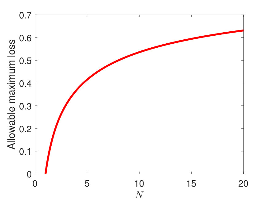 Figure 1
 Figure 2
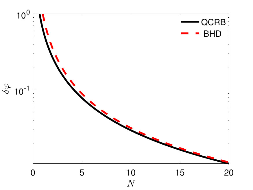 Figure 3
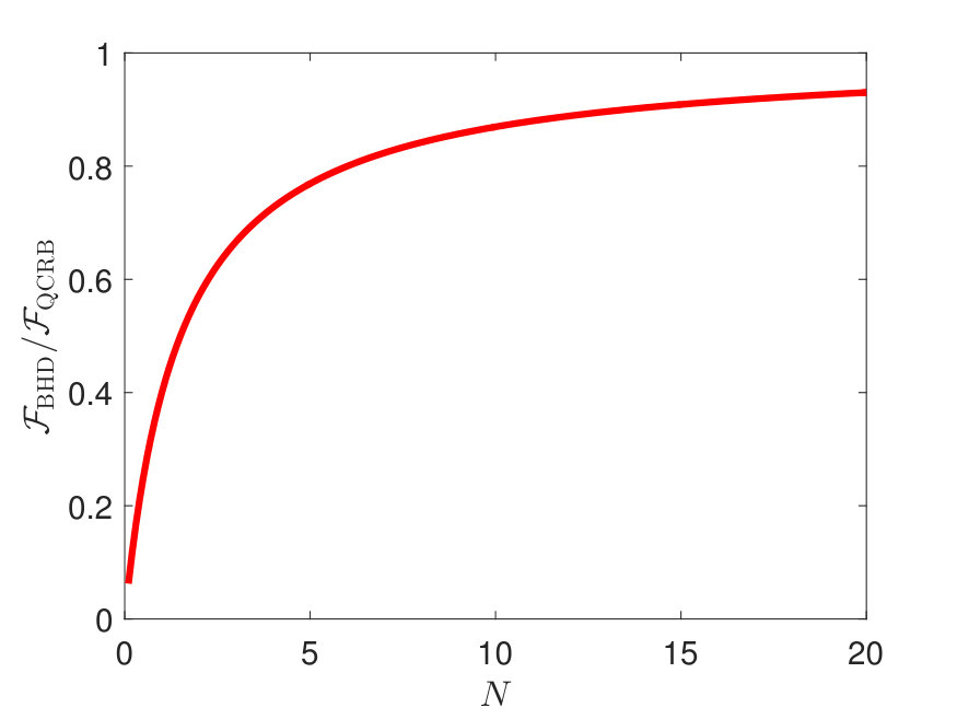 Figure 4
 Figure 5
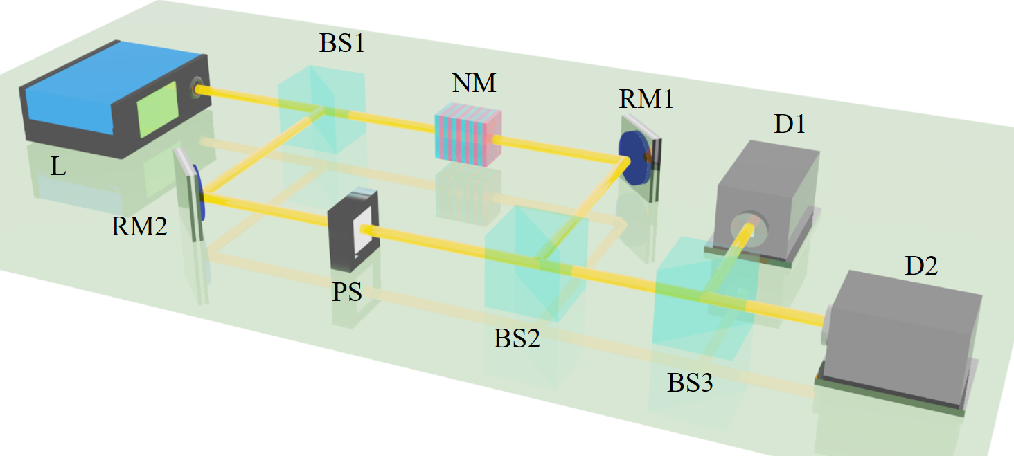 Figure 6
 Figure 7
 Figure 8
 Figure 9
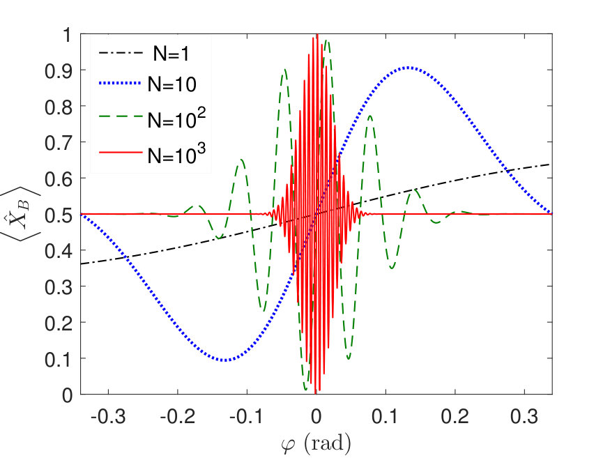 Figure 10
 Figure 11
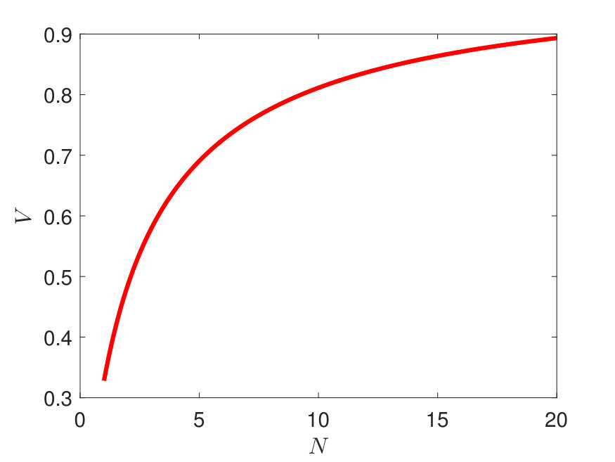 Figure 12
Peer Reviews
No public reviews on file for this paper yet. If you reviewed it on a platform where reviews are public (OpenReview, ICLR, NeurIPS, ICML), you can paste yours below so the community can read it here.
Videos
No videos yet. Explain this paper in a talk, walkthrough, or lecture? Add one.
Taxonomy
TopicsQuantum Information and Cryptography · Quantum Mechanics and Applications · Mechanical and Optical Resonators
A nearly optimal and robust protocol for nonlinear phase estimation using coherent states
Jian-Dong Zhang
School of Physics, Harbin Institute of Technology, Harbin 150001, China
Zi-Jing Zhang
School of Physics, Harbin Institute of Technology, Harbin 150001, China
Jun-Yan Hu
School of Physics, Harbin Institute of Technology, Harbin 150001, China
Long-Zhu Cen
School of Physics, Harbin Institute of Technology, Harbin 150001, China
Yi-Fei Sun
School of Physics, Harbin Institute of Technology, Harbin 150001, China
Chen-Fei Jin
School of Physics, Harbin Institute of Technology, Harbin 150001, China
Yuan Zhao
School of Physics, Harbin Institute of Technology, Harbin 150001, China
Abstract
We propose a protocol for the second-order nonlinear phase estimation with a coherent state as input and balanced homodyne detection as measurement strategy. The sensitivity is sub-Heisenberg limit, which scales as for photons on average. By ruling out hidden resources in quantum Fisher information, the fundamental sensitivity limit is recalculated and compared to the optimal sensitivity of our protocol. In addition, we investigate the effect of photon loss on sensitivity, and discuss the robustness of measurement strategy. The results indicate that our protocol is nearly optimal and robust.
I Introduction
Within the past two decades, quantum technologies have developed at an unheard-of rate. There are a great deal of revolutionary progresses in proof-of-principle experiments, offering an insight into world from microscopic view. As a momentous component of quantum technologies, quantum metrology Giovannetti et al. (2006); Taylor and Bowen (2016) is a science that exploits exotic quantum resources to enhance estimation precision of physical quantities. In this regard, quantum-enhanced interferometers come across as a suitable tool and play a paramount role. They work by mapping a small variation of interest onto an unknown relative phase shift between the two arms and by estimating this phase.
In recent years, linear phase estimation has received a boost with an influx of demands from the rapidly developing field of quantum information processing. Exotic input states and novel measurement strategies have aroused wide interests, so long as they are capable of breaking the shot-noise limit or Rayleigh diffraction limit. Among these inputs, two-mode squeezed vacuum and entangled coherent states are probably the greatest candidates, which can even surpass the Heisenberg limit. Regarding measurement strategies, parity, on-off, and projective measurements have shown extraordinary performances—optimal or robust or both—in different scenarios.
As another important element, nonlinear processes also are of vital significance. Many of the exotic quantum resources are produced during nonlinear light-matter interactions, e.g., preparations for squeezed and superposition states Eckstein et al. (2011); Takahashi et al. (2008). Related to this, nonlinear phase estimation has also gained lots of attention Rivas and Luis (2010); Cheng (2014); Joo et al. (2012); Gerry et al. (2002); Kitagawa and Yamamoto (1986); Berrada (2013); Luis and Rivas (2015). However, most of these protocols only provide the sensitivity limits calculated from the quantum Fisher information (QFI). That is, the optimal measurement strategy saturating the QFI is not provided. Furthermore, the QFI-only calculation may be a loosen lower bound, since it is on the cards that some hidden resources dilute the tightness. Hence, there are some gaps to be filled in this respect, and one needs to study those protocols containing specific measurement strategy. To this end, here we propose a estimation protocol for nonlinear phase shifts through the use of coherent states and balanced homodyne detection. The QFI is recalculated via the phase-averaging approach, in which any hidden resources are eliminated Jarzyna and Demkowicz-Dobrzański (2012); Takeoka et al. (2017); You et al. (2019).
II Estimation protocol
We start off with the introduction of our estimation protocol. Consider a Mach-Zehnder interferometer as depicted in Fig. 1, a nonlinear medium and a phase shifter are inserted into its two paths. The clockwise and counterclockwise paths are labeled as spatial modes and , respectively. Throughout this paper, () and () stand for the creation and annihilation operators in mode (). The phase shifter is used to offset the linear phase induced by the nonlinear medium. The first input port is fed by a coherent state generated by a laser, and the second one is empty. Thus, the input state can be delineated as . Upon leaving the first 50-50 beam splitter, this state goes to .
Without loss of generality, the th-order nonlinear phase operator can be described as with respect to nonlinear phase . The linear phase is phase difference between the two modes after compensation by the phase shifter. For simplicity, we consider the scenario that the linear phase is only in mode ; accordingly, the state after experiencing phase shift becomes
[TABLE]
Finally, this state is incident on the second 50-50 beam splitter, and balanced homodyne detection is performed at the output.
III Measurement and estimation in a lossless scenario
Balanced homodyne detection was originally developed by Yuen and Chan Yuen and Chan (1983). It is a process, by which the output state is mixed with a phase-tunable local oscillator, which itself is a coherent state of the same frequency as the input. In Fig. 1, the local oscillator is injected into the third 50-50 beam splitter, and is not shown for simplicity. This measurement strategy is a standard technique for quantum noise detection by detecting quadrature-phase or quadrature-amplitude. For Gaussian inputs, even without a photon-number-resolving detector, one can utilize this strategy to measure the parity of the output Plick et al. (2010).
Consider the quadrature of path , the measurement operator can be expressed as , and the expectation value of this operator is equal to
[TABLE]
Where the sequitur derived from the Baker-Hausdorff lemma is used, and the operator of 50-50 beam splitter is given by .
The expectation value of the first term in Eq. (2) is found to be
[TABLE]
here we assume that the parameter is a positive real number. Regarding the second term, it can be calculated through the use of the lemma Louisell (1973). We decompose the nonlinear phase term into
[TABLE]
where the term is ignored since it denotes a linear phase shift. By means of the above lemma, we have
[TABLE]
with operator . Further, using the lemma Louisell (1973), we can obtain the expectation value of the second term in Eq. (2),
[TABLE]
with being the mean photon number inside the interferometer. Substituting Eq. (2) by Eqs. (3) and (6), the expectation value of quadrature is obtained
[TABLE]
and that of the square of quadrature turns out to be
[TABLE]
Based on Eqs. (7) and (8), the optimal sensitivity of phase is given by
[TABLE]
Equation (9) manifests that the sensitivity gets its optimal value when the conditions and are satisfied. It should be noted that here is the solution of equation . The relationship between and is given by Eq. (7) Zhang et al. (2018).
To observe the behavior of the expectation value, in Fig. 2(a) we plot the normalized expectation value as a function of the nonlinear phase shift. Figure 2(a) suggests that the full width at half maximum gets narrow with the increase of the mean photon number; meanwhile, there exist multi-fold oscillating fringes in an envelope. These narrow fringes originate mainly from the exponential term . The envelope is modulated by the sine term , and the oscillation corresponds to the term in the sine function. According to the definition of visibility Dowling (2008)
[TABLE]
in Fig. 2(b) we give dependence of the visibility of our protocol on the mean photon number. With increasing the photon number, the visibility increases at a quick rate. We can get the expectation value of which the visibility is in exceed of 90% so long as the number of photons is greater than 20.
IV Fundamental sensitivity limit
In the last section, we have calculated the sensitivity of our protocol. For evaluating the optimality of measurement strategy, in this section, we give the QFI and compare it with our sensitivity. Of the linear phase estimation, the QFI-only calculation may loosen the tightness of sensitivity limit. For SU(2) interferometers, using operators and to describe the estimated phase , one may get two different QFI with respect to the same inputs. Consider a coherent state and a vacuum as inputs, the QFI of the former is and that of the latter is Jarzyna and Demkowicz-Dobrzański (2012); Takeoka et al. (2017). Regarding SU(1,1) interferometers, there exist a large number of similar situations. With the same input states, two different QFI may be obtained if one uses operators and to describe the phase shift You et al. (2019). That is, two different sensitivity limits may be obtained from the same physical configurations. To circumvent this overestimation, some studies capitalize on the phase-averaging approach to calculate the QFI; accordingly, this problem is partially resolved by this approach in both SU(2) and SU(1,1) interferometers. The detailed discussions can be found in Refs. Jarzyna and Demkowicz-Dobrzański (2012); Takeoka et al. (2017); You et al. (2019).
Due to the above reasons, here we deploy the phase-averaging approach to calculate the QFI. For our protocol, the density matrix for the input state can be written as
[TABLE]
in twin Fock basis, where . According to the phase-averaging approach, we need to erase the phase reference information, and then the input turns to a mixed state from a pure state,
[TABLE]
After the first beam splitter, this density matrix evolves into
[TABLE]
with the state
[TABLE]
The above state is a pure state and obeys the orthogonality . Related to this, the relationship between total QFI and the QFI of the state in Eq. (14) is given by
[TABLE]
In order to calculate , we give normal order of the estimator and that of its square . For the state , the expectation value of normal order can be calculated by
[TABLE]
Further, the QFI of the state is equal to
[TABLE]
Combining Eqs. (15) and (17), the total QFI can be expressed as
[TABLE]
The corresponding sensitivity limit is calculated via the equation .
Figure 3(a) demonstrates the quantum Cramér-Rao (QCR) bound—inverse square root of the QFI—and the optimal sensitivity obtained by our protocol, respectively. For the region of small photon number, the sensitivity is slightly inferior to the bound. With further increasing the number of photons, the sensitivity approaches the QCR bound. This reveals that balanced homodyne detection is a nearly optimal strategy. In Fig. 3(b), we present the normalized available Fisher information, . This quotient describes the degree of optimality, only when the optimal strategy is performed does the quotient sit at 1. From the figure we can find that balanced homodyne detection continuously approaches the optimal strategy with increasing the mean photon number.
V Lossy effect on estimation protocol
In general, realistic interferometers need to deal with a trade-off among the optimality, robustness, and complexity. For our protocol, there is needless to excessively anxious about the complexity, since a conventional interferometer can be competent. Regarding the optimality, we have proved that balanced homodyne detection is a nearly optimal measurement strategy, which approaches the QCR bound. Thus, in this section we briefly discuss the robustness of our protocol, the effect of photon loss on the optimal sensitivity is considered.
For simplicity, we merely discuss the same losses in the two paths. Photon loss is usually modeled by inserting a fictitious beam splitter with transmissivity and reflectivity . For a single-mode state, the reflected photons enter the surrounding thermal bath, known as photon loss. The first scenario we consider is the photon loss before the nonlinear phase shift, at this point the amplitude of the coherent state becomes . As a consequence, the expectation value of quadrature reduces to
[TABLE]
and that of its square is expressed as
[TABLE]
with . Based on above calculation results, we have the optimal sensitivity, , which equals the sensitivity of a lossless interferometer fed by a coherent state with the mean photon number .
Similarly, for the second scenario—photon loss after the nonlinear phase shift—we get the expectation values,
[TABLE]
Using Eqs. (21), (22) and error propagation, the optimal sensitivity is obtained. An interesting phenomenon is that the optimal sensitivities of the two scenarios are the same, although the sensitivities are not equal for . Therefore, with respect to the optimal sensitivity, the places where the photon loss occurs are unimportant, .
Under the scenario of photon loss, only if the lossy ratio is less than can the sensitivity break the Heisenberg limit, and here is called as the allowable maximum loss. In Fig. 4, we describe the relationship between the allowable maximum loss and mean photon number. It can be seen that the allowable maximum loss increases rapidly with the increase of mean photon number. The protocol can achieve sub-Heisenberg-limited sensitivity and withstand the photon loss in exceed of 60% for . This implies that our protocol is robust, and the robustness can be improved by increasing the photon number.
VI Conclusion
This paper focuses on an estimation protocol for the second-order nonlinear phase shifts. The input is a coherent state combined with a vacuum, and balanced homodyne detection is performed onto one of the two outputs. In a lossless scenario, we get sub-Heisenberg-limited sensitivity scaling of , and the output visibility is superior to 90% with . By taking advantage of the phase-averaging approach, we rule out the virtual component of the QFI brought by hidden resources, and ascertain the fundamental sensitivity limit. Compared with this fundamental limit, the sensitivity of our protocol is approximately saturated. As a realistic consideration, photon loss is discussed in two scenarios, before and after the nonlinear phase shift. The results point out that the optimal sensitivities of these two scenarios are the same; furthermore, the effect of photon loss on the sensitivity is not serious. For the region of , our protocol stands up to the photon loss in exceed of 60% and, meanwhile, achieves the Heisenberg limit. Overall, our protocol is of approximate optimality and robustness for nonlinear phase estimation.
The reference list from the paper itself. Each links out to its DOI / PubMed record.
- 1Giovannetti et al. (2006) V. Giovannetti, S. Lloyd, and L. Maccone, Phys. Rev. Lett. 96 , 010401 (2006) . · doi ↗
- 2Taylor and Bowen (2016) M. A. Taylor and W. P. Bowen, Phys. Rep. 615 , 1 (2016) .
- 3Eckstein et al. (2011) A. Eckstein, A. Christ, P. J. Mosley, and C. Silberhorn, Phys. Rev. Lett. 106 , 013603 (2011) . · doi ↗
- 4Takahashi et al. (2008) H. Takahashi, K. Wakui, S. Suzuki, M. Takeoka, K. Hayasaka, A. Furusawa, and M. Sasaki, Phys. Rev. Lett. 101 , 233605 (2008) . · doi ↗
- 5Rivas and Luis (2010) A. Rivas and A. Luis, Phys. Rev. Lett. 105 , 010403 (2010) . · doi ↗
- 6Cheng (2014) J. Cheng, Phys. Rev. A 90 , 063838 (2014) . · doi ↗
- 7Joo et al. (2012) J. Joo, K. Park, H. Jeong, W. J. Munro, K. Nemoto, and T. P. Spiller, Phys. Rev. A 86 , 043828 (2012) . · doi ↗
- 8Gerry et al. (2002) C. C. Gerry, A. Benmoussa, and R. A. Campos, Phys. Rev. A 66 , 013804 (2002) . · doi ↗