This paper introduces a new Bernstein likelihood estimation method for proportional hazard models with interval-censored data, providing smoother survival estimates and improved regression coefficient accuracy.
Contribution
It proposes a maximum approximate Bernstein likelihood approach that enhances estimation of baseline density and regression coefficients in interval-censored survival analysis.
Findings
01
Faster convergence rate for survival function estimates
02
Better finite sample performance than existing methods
03
Effective real data application demonstration
Abstract
Maximum approximate Bernstein likelihood estimates of the baseline density function and the regression coefficients in the proportional hazard regression models based on interval-censored event time data are proposed. This results in not only a smooth estimate of the survival function which enjoys faster convergence rate but also improved estimates of the regression coefficients. Simulation shows that the finite sample performance of the proposed method is better than the existing ones. The proposed method is illustrated by real data applications.
Figures4
Click any figure to enlarge with its caption.
Figure 1
Figure 2
Figure 3
Figure 4
Tables1
Table 1. Table 1: Mean squared errors of estimates of the regression coefficients using semiparametric method (SP), the proposed method using m = m ~ 𝑚 ~ 𝑚 m=\tilde{m} (B1), the proposed method using m = m ^ 𝑚 ^ 𝑚 m=\hat{m} (B2), and the parametric method (P).
No public reviews on file for this paper yet. If you reviewed it on a platform where reviews are public (OpenReview, ICLR, NeurIPS, ICML), you can paste yours below so the community can read it here.
Videos
No videos yet. Explain this paper in a talk, walkthrough, or lecture? Add one.
Taxonomy
TopicsStatistical Methods and Inference · Control Systems and Identification · Fuzzy Systems and Optimization
Full text
Maximum Approximate Bernstein Likelihood Estimation in Proportional Hazard Model for Interval-Censored Data
Maximum approximate Bernstein likelihood
estimates of the baseline density function and the regression coefficients in the
proportional hazard regression models based on interval-censored
event time data are proposed. This results in not only a smooth estimate of the
survival function which enjoys faster convergence rate but also improved estimates of
the regression coefficients. Simulation shows that the finite sample performance of the proposed
method is better than the existing ones. The proposed method is illustrated by real data
applications.
Key Words and Phrases: Approximate Likelihood, Bernstein Polynomial Model, Cox’s Proportional Hazard Regression Model, Density Estimation,
Interval Censoring, Survival Curve.
1 Introduction
Traditionally in semi- and nonparametric statistics we approximate an unknown smooth distribution function by a step function and parameterize this infinite-dimensional parameter by the jump sizes of the step function at the observed values. Therefore, the working model is actually of finite but varying dimension.
The resulting estimate is a step function and does not deserve a density. This approach works fine when the infinite-dimensional parameter is nuisance. However, in the situation when such parameters such as survival, hazard, and density functions are our concerns the traditional approach which results in a jagged step-function estimation is not satisfactory especially when sample size is small which is usually the case for survival analysis of rare diseases. Besides the roughness of the estimation when data are incompletely observed it is difficult to parameterize the unknown survival function and not easy to find the nonparametric maximum likelihood estimate due to the complication of assigning probabilities and the large number of parameters (usually the same as the sample size) to be estimated. Moreover, the roughness of the estimate of nonparametric component could reduce the accuracy of the estimates of parameters in semiparametric models. Turnbull, (1976) presented an EM algorithm (Dempster et al.,, 1977) to compute the discrete nonparametric maximum likelihood estimate (NPMLE) of the distribution function from grouped, censored, and truncated data without covariates (see also Groeneboom and Wellner,, 1992). The method is generalized to obtain semiparametric maximum likelihood estimate (SPMLE) of the survival function to models including Cox’s proportional hazards (PH) model by Finkelstein, (1986), Huang, (1996), Huang and Wellner, (1997), and Pan, (1999). Finkelstein and Wolfe, (1985) proposed some semiparametric models for interval censored data. Asymptotic results about some semiparametric models can be found in Huang and Wellner, (1997), and Schick and Yu, (2000), etc. With interval censored data the assignment of the probabilities within the Turnbull interval cannot be uniquely determined (Anderson-Bergman, 2017b, ). Groeneboom and Wellner, (1992) suggested an iterative convex minorant (ICM) algorithm, which was improved or generalized by
Wellner and Zhan, (1997), Pan, (1999), and Anderson-Bergman, 2017a . Grouped failure time data have been studied by, among others, Prentice and Gloeckler, (1978) and Pierce et al., (1979). Unfortunately, the NPMLE or SPMLE of the survival function
is a step-function and may be not unique. Parametric models and Kernel smoothing methods (Parzen,, 1962; Rosenblatt,, 1956) have been applied to obtain smooth estimator of survival function (Lindsey,, 1998; Lindsey and Ryan,, 1998; Betensky et al.,, 1999).
Another continuous estimation was due to Becker and Melbye, (1991) who assumed piecewise
constant intensity model.
Carstensen, (1996) generalized this method to regression models by assuming piecewise constant baseline rate.
Goetghebeur and Ryan, (2000) indicated that many of the EM-like methods have the relatively ad hoc nature of the procedure used to impute missing data and proposed a method using approximate likelihood to avoid such problem that retains some of the appealing features of the nonparametric smoothing methods such as the regression spline smoothing of Kooperberg and Clarkson, (1998) and the local likelihood kernel smoothing of Betensky et al., (1999).
Nonparametric density estimation is rather difficult due the lack of information contained in sample about it (Bickel et al.,, 1998; Ibragimov and Khasminskii,, 1983). Kernel method is usually unsatisfactory when sample size is small
even for complete data. Some authors have studied the estimation of density function based on censored data (see for example Braun et al.,, 2005; Harlass,, 2016, and the refereces therein) without covariate.
A useful working statistical model must be finite-dimensional and approximates (see page 1 of Bickel et al.,, 1998) the true underlying distribution. Instead of approximating the underlying continuous distribution function by a step-function which is a multinomial probability model, Guan, (2016) suggested a Bernstein polynomial approximation (Bernstein,, 1912; Lorentz,, 1963) which is actually a mixture of some specific beta distributions. This Bernstein polynomial model performs much better than the classical kernel method for estimating density even from grouped data (Guan,, 2017). The maximum approximate Bernstein likelihood estimate can be viewed as a continuous version of the NPMLE or SPMLE.
In this paper such estimates of the conditional survival and density functions given covariate are proposed by fitting interval censored data with Cox’s proportional hazards model.
2 Methodology
2.1 Proportional Hazards Model
Let T be an event time and X be an associated d-dimensional covariate with distribution H(x) on X. We denote the marginal and the conditional survival functions of T, respectively, by
S(t)=Fˉ(t)=1−F(t)=P(T>t) and S(t∣x)=Fˉ(t∣x)=1−F(t∣x)=P(T>t∣X=x).
Let f(t∣x) denote the conditional density of a continuous T given X=x. The conditional cumulative hazard function, odds ratio, and hazard rate are, respectively,
[TABLE]
Consider the Cox’s proportional hazard (PH) regression model (Cox,, 1972)
[TABLE]
where γ∈Γ⊂Rd, x~=x−x0, x0 is any fixed covariate value, f0(⋅)=f(⋅∣x0) is the unknown baseline density and S(⋅∣x0)=∫⋅∞f(t∣x0)dt is the corresponding survival function.
This is equivalent to
[TABLE]
It is clear that (1) and (2) are also true if we change the “baseline” covariate x0 to any x0∗∈X with the same γ but x~ being replaced by x~∗=x−x0∗.
For a given γ∈Γ, define a γ-related “baseline” as an xγ∈argminx∈Xγ⊤x and denote x~γ=x−xγ.
Define τ=inf{t:F(t∣x0)=1}.
It is true that τ is independent of x0, 0<τ≤∞, and f(t∣x) have the same support [0,τ] for all x∈X.
It is obvious that for any strictly increasing continuous function ψ, P(ψ(T)>t∣x)=P(ψ(T)>t∣x0)exp(γ⊤x~).
Thus the transformed event time ψ(T) also satisfies the Cox model (1).
We will consider the general situation where the event time is subject to interval censoring. The observed data are Z=(Y,X,Δ), where Y=(Y1,Y2] and Δ is the censoring indicator, i.e., T=Y=Y1=Y2 is uncensored if Δ=0 and T∈Y=(Y1,Y2], 0≤Y1<Y2≤∞, is interval censored if Δ=1.
The reader is referred to Huang and Wellner, (1997) for a review and more references about interval censoring.
The right-censoring Y2=∞
and left-censoring Y1=0 are included as special cases.
For any individual observation z=(y,x,δ), where if δ=0 then y=y=t else if δ=1 then y=(y1,y2]∋t, 0≤y1<y2≤∞, the full loglikelihood, up to an additive term independent of (γ,f0), is
[TABLE]
Let (yi,xi,δi), i∈I1n be independent observations of (Y,X,Δ), here and in what follows Imn={m,…,n} for any integers m≤n≤∞. If τ is either unknown or τ=∞ and τn is at least the last finite observed time, i.e., τn≥y(n)=max{yi1,yj2:yj2<∞;i,j∈I1n} then [τn,∞) is contained in the last Turnbull interval (Turnbull,, 1976). It is well known that if the last event time is right censored then the distribution of T is not “nonparametrically estimable” on [τn,∞). Thus all finite observed times are in [0,τn] and we can only estimate the truncated version of f(t∣x) on [0,τn], fˉ(t∣x)=f(t∣T∈[0,τn],x)=f(t∣x)/F(τn∣x), t∈[0,τn]. In many applications with right censored last observation fˉ(t∣x) does not approximate f(t∣x) because F(τn∣x) may be not close to one.
2.2 Approximate Bernstein Polynomial Model
The full likelihood (3) cannot be maximized without specifying S(t∣x0) using a finite dimensional model.
Traditional method approximates S(t∣x0) by step-function and treats the jumps at observations as unknown parameters. For censored or other types of incompletely observed data this parametrization is difficult and complicated. However the Bernstein polynomial approximation makes the parametrization simple and much easy (Guan,, 2016, 2017).
Given any x0, we approximate the truncated density fˉ(t∣x0)=f(t∣x0)/F(τn∣x0) by
fˉm(t∣x0;pˉ)=τn−1∑i=0mpˉiβmi(t/τn), a mixture of beta densities βmi with shape parameters (i+1,m−i+1), i∈I0m, and unknown mixing proportions pˉ=pˉ(x0)=(pˉ0,…,pˉm). Here the dependence of pˉ=pˉ(x0) on x0 will be suppressed.
The mixing proportions pˉ
are subject to constraints pˉ∈Sm≡{(u0,…,um)⊤∈Rm+1:ui≥0,∑i=0mui=1.}.
Denote π=π(x0)=F(τn∣x0).
Reparametrizing with pi=πpˉi, i∈I0m, we can approximate f(t∣x0) on [0,τn] by fm(t∣x0;p)=π(x0)fˉm(t∣x0;p)=τn1∑i=0mpiβmi(t/τn).
If π<1, although we do not need and cannot estimate the values of f(t∣x0) on (τn,∞), we can put an arbitrary guess on them such as
fm(t∣x0;p)=pm+1α(t−τn), t∈(τn,∞), where pm+1=1−π and α(⋅) is a density on [0,∞) such that (1−π)α(0)=(m+1)pm/τn so that fm(t∣x0;p) is continuous at t=τn, e.g., α(t)=α(0)exp[−α(0)t]. Thus f(t∣x0) and S(t∣x0) on [0,∞), can be “approximated”, respectively, by
[TABLE]
and
[TABLE]
where Bˉmi(t)=1−Bmi(t)=1−∫0tβmi(s)ds, i∈I0m, Bˉm,m+1(t)≡1, and Aˉ(t)=∫t∞α(u)du. Thus we can approximate S(t∣x) and f(t∣x) on [0,τn], respectively, by
[TABLE]
If τ is finite and known we choose τn=τ and specify pm+1=0. Otherwise, we choose τn=y(n). In this case, from (3) we see that for data without right-censoring and covariate
we have to specify pm+1=0 due to its unidentifiability.
If τn=1 we divide all the observed times by τn. Thus we assume τn=1 in the following.
We define m∗=m or =m+1 according to whether we specify pm+1=0 or not. Thus p=(p0,…,pm∗) and satisfies constraints
[TABLE]
The loglikelihood
ℓ(γ,f0;z) can be approximated by
the Bernstein loglikelihood ℓm(γ,p;z)=ℓ(γ,fm(⋅∣x0;p);z), that is,
[TABLE]
where Sm(∞∣x0;p)=0.
The loglikelihood
ℓ(γ,f0)=∑i=1nℓ(γ,f0;zi)
can be approximated by
[TABLE]
For a given degree m, if (γ^,p^) maximizes ℓm(γ,p) subject to constraints in (8) for some x0 then (γ^,p^) is called the maximum approximate Bernstein (or beta) likelihood estimator (MABLE) of (γ,p). This is a full likelihood method. The MABLE’s of f(t∣x) and S(t∣x) are, respectively,
[TABLE]
The derivative of ℓm(γ,p;z) with respect to p is
[TABLE]
where, for j∈I0m∗,
[TABLE]
Lemma 1**.**
The Hessian matrix H(γ,p)=∂p∂p⊤∂2ℓm(γ,p) is nonpositive, i.e., all entries are nonpositive. For any fixed γ if γ⊤x0≤min1≤i≤n{γ⊤xi} then H(γ,p) is negative semi-definite for each p∈Sm∗. If, in addition, the vectors [Ψj(γ,p;z1), …,Ψj(γ,p;zn)], j∈I0m∗, are linearly independent, then H(γ,p) is negative definite.
Let p~=p~(γ)=(p~0,…,p~m∗)⊤ denote the maximizer of ℓm(γ,p) with respect to p=(p0,…,pm∗)⊤ subject to constraints in (8).
Similar to Peters, Jr. and Walker, (1978) we have the following result about a necessary and sufficient condition for p~.
Theorem 1**.**
For any fixed γ if γ⊤x0≤min1≤i≤n{γ⊤xi} then p~=p~(γ) is a maximizer of ℓm(γ,p) if and only if
[TABLE]
for all j∈I0m∗ with equality if p~j>0. If, in addition, the vectors [Ψj(γ,p;z1), …,Ψj(γ,p;zn)], j∈I0m∗, are linearly independent for all p in the interior of Sm∗, then p~ is unique.
So it is necessary that
p~j=p~jΨˉj(γ,p~), j∈I0m∗,
where
[TABLE]
We have fixed-point iteration
[TABLE]
If γ⊤x0≤min1≤i≤n{γ⊤xi} then Ψˉj(γ,p)≥0 for all j∈I0m∗
and p∈Sm∗.
Similar to the proof of Theorem 4 of Peters, Jr. and Walker, (1978) we can prove the convergence of p[s].
Theorem 2**.**
For any fixed γ suppose γ⊤x0≤min1≤i≤n{γ⊤xi}. If p[0] is in the interior of Sm∗, the sequence {p[s]} of (13) converges to p~.
Define an empirical γ-related “baseline” x^0=x^0(γ) such that γ⊤x^0=min1≤i≤n{γ⊤xi}.
Lemma 2**.**
The matrix ∂γ∂γ⊤∂2ℓm(γ,p) is negative definite.
Let γ~ be an efficient estimator of γ such as the NPMLE and SPMLE. We choose x0=x^0(γ~).
Then we maximize ℓm(γ~,p) to obtain p~=p~(γ~).
Therefore we can estimate
f(t∣x) and S(t∣x) on [0,1], respectively, by
[TABLE]
For the data without covariate, we have γ^=0. Then we have f^B(t)=fm(t∣x;0,p^) and S^B(t)=Sm(t∣x;0,p^).
For the NPMLE or SPMLE γ~ of γ, the profile estimates (γ~,p~) are close to (γ^,p^) especially for large sample size. Thus (γ~,p~) can be used as initial values to find (γ^,p^) by the following algorithm. Such procedure was also suggested by Huang, (1996).
Step 0:
Start with an initial guess γ(0) of γ.
Choose x0(0)=x^0(γ(0)). Use (13) with γ~=γ0, x0=x0(0), and starting point p[0]=um≡(1,…,1)/(m∗+1) to get p(0)=p~.
Set s=0
Step 1:
Find the maximizer γ(s+1) of ℓm(γ,p(s)) using the Newton-Raphson method.
Step 2:
Choose x0(s+1)=x^0(γ(s+1)) and γ~=γ(s+1). If γ~⊤Δx0≡γ~⊤(x0(s+1)−x0(s))=0 then p[0]=p(s) otherwise pi[0]=Cmfm(i/m∣x0(s+1);γ~,p(s)), i∈I0m, pm+1[0]=(pm+1(s))eγ~⊤Δx0 if m∗=m+1, where Cm is chosen so that ∑i=0mpi[0]=1−pm+1[0]. Then use (13) with x0=x0(s+1) to get p(s+1)=p~. If the so obtained p[0] is not in the interior of Sm∗ we set p[0]=(p[0]+ϵum)/(1+ϵ) using a small ϵ>0. Set s=s+1.
Step 3:
Repeat Steps 1 and 2 until convergence. The final γ(s) and p(s) are taken as the MABLE (γ^,p^) of (γ,p) with baseline x^0=x0(s).
The concavities of ℓm(γ,p) with respect to γ and p ensure that the above iterative algorithm is a point-to-point map and the solution set contains single point.
Convergence of (γ(s),p(s)) to (γ^,p^) is guaranteed by the Global Convergence Theorem (Zangwill,, 1969).
2.2.1 Some Special Cases
Data Without Covariate:
For interval-censored data without covariate, zi=(yi,δi), i∈I1n. The iteration (13) reduces to
[TABLE]
where
[TABLE]
fm(t;p)=∑j=0mpiβmj(t), and Sm(t;p)=∑j=0m∗pjBˉmj(t).
Two-Sample Data:
When x=x is binary, x=1 for cases and x=0 for controls, we have
a two-sample PH model which specifies S(t∣1)=[S(t∣0)]exp(γ).
In this case,
usually γ≥0 so that Ψj(γ,p;z) is always positive for each j.
In case γ<0 we switch case and control data.
2.3 Model Selection
The change-point method for model degree selection (Guan,, 2016) applies for finding an optimal degree m for a given regression model.
Let M={m0,…,mk}, mi=m0+i, i∈I0k. For each i∈I0k, fit the data to obtain (γ^,p^) and ℓi=ℓmi(γ^,p^).
The optimal degree m is the maximizer m^ of
[TABLE]
where R(mk)=0. Alternatively, we can replace ℓi by ℓmi(γ~,p~) where p~=p~(γ~) for a fixed efficient estimate γ~ for all i. The resulting optimal degree is denoted by m~. Then using m=m^ or m=m~ we obtain (γ^,p^).
3 Asymptotic Results
3.1 Some Assumptions and Conditions
The following assumptions are needed to develop asymptotic theory.
(A1)****.
The support X of covariate X is compact and for each x0∈X, E(X~X~⊤) is positive definite, where X~=X−x0.
(A2)****.
For each x0∈X and τn>0, there exist fm(t∣x0;p0)
and ρ>0 such that,
uniformly in t∈[0,τn],
[TABLE]
where p0=(p01,…,p0m,p0,m+1)⊤, p0i=π(x0)pˉ0i, i∈I0m, p0,m+1=1−π(x0)=S(τn∣x0).
For any γ, the compactness of X ensures the existence of xγ∈argmin{γ⊤x:x∈X}. Boundedness of X is assumed in the literature, e.g. (A3)(b) of Huang and Wellner, (1997). The positive finiteness of E(X~X~⊤) assures the identifiability of γ.
Let C(r)[0,1] be the class of functions which have rth continuous derivative f(r) on [0,1]. A function f is said to be α–Hölder
continuous with α∈(0,1] if ∣f(x)−f(y)∣≤C∣x−y∣α for some constant C>0. We have the following result.
Lemma 3**.**
Suppose that φ(t)=ta(1−t)bφ0(t) is a density on [0,1], a and b are nonnegative integers, φ0∈C(r)[0,1], r≥0, φ0(t)≥b0>0, and φ0(r) is α-Hölder
continuous with α∈(0,1].
Then there exists p0∈Sm such that uniformly in t∈[0,1], with ρ=r+α,
[TABLE]
This lemma was proved in Wang and Guan, (2019).
This is a generalization of the result of Lorentz, (1963) which requires a positive lower bound for φ, *i.e. *, a=b=0.
If φ(t)=τnfˉ(τnt∣x0)=τnf(τnt∣x0)/π(x0) as a density on [0,1] fulfills the condition of Lemma 3, then
assumption (A2) is fulfilled.
The condition of Lemma 3 seems only sufficient for (A2).
In the following, all expectations E(⋅) are taken with respect to the (joint) distribution of random variable(s) in upper case.
The following are the conditions for cases considered in the asymptotic results.
(C0)****.
The event time T is uncensored and τn=τ<∞.
(C1)****.
The event time T is subject to Case 1 interval censoring.
Given X=x the inspection time Y has cdf G1(⋅∣x) on [τl,τu], 0<τl<τu=τn<τ≤∞, and
[TABLE]
(C2)****.
The event time T is subject to Case k (k≥2) interval censoring
Given X=x the observed inspection times Y=(Y1,Y2) have joint cdf G2(⋅,⋅∣x) on {y=(y1,y2):0<τl≤y1≤y2≤τu}, τn=τu<τ, and
[TABLE]
where G21 is the marginal cdf of Y1.
The condition about the support of the inspection times are similar to those of Huang and Wellner, (1997).
The next theorem is about the identifiability of the approximate model.
Theorem 3**.**
Suppose that X is almost surely linearly independent on X. Then for uncensored data both γ and p are identifiable. For censored data, if, in addition, the inspection time is continuous then both γ and p are identifiable.
3.2 Some Statistical Distances
Under condition (C0), define statistical distances
[TABLE]
where γ0 is the true value of γ.
Under condition (C1), we define a weighted version of the Anderson and Darling, (1954) distance as
In the following the same symbols C and C′ may represent different constants in different places.
Theorem 4**.**
Let (γ^,p^) be the MABLE of (γ,p) with degree m≥Cn1/ρ for some constant C>0. Suppose that assumptions (A1) and (A2) are satisfied. For each i=0,1,2, and any ϵ∈(0,1/2), under condition (C i), we have
∥γ^−γ0∥2≤Cn−1+ϵ, a.s. and
Di2(p^;x^0)≤Cn−1+ϵ, a.s..
Theorem 5**.**
Suppose that assumptions (A1) and (A2) are satisfied. Let γ~=γ~(p0) be the maximizer of ℓm(γ,p0) for some p0 that satisfies (A2).
For each i=0,1,2, under condition (C i), n(γ~−γ0) converges in distribution to N(0,I−1) as n→∞, where x0∈argminx∈Xγ0⊤x, I=E(X~X~⊤) under condition (C0); I=E{[O(Y∣X)Λ2(Y∣X)]X~X~⊤} under condition (C1); and
For Cox’s maximum partial likelihood estimator γ^cox from uncensored data, the information is
[TABLE]
By the law of total covariance
[TABLE]
with equality iff E(X∣T=t) is constant.
So under this surreal situation, the information I=E(X~⊗2)≥Icox for all x0∈X. More theoretical work need be done to access the information loss due to the unknown p0.
Because ℓm(γ,p) depends on p through fm(⋅∣x0;p) and fm(⋅∣x0;p0)≈fm(⋅∣x0;p^), although p0 is unknown, we have γ^≈γ~.
We can estimate the information I by, with x0=x^0,
[TABLE]
4 Simulation
Assume that given X=x, T is Weibull W(θ,σe−γ⊤x/θ) so that the baseline x=0 distribution is W(θ,σ) with shape and scale θ=σ=2.
The function simIC_weib() of R package icenReg (Anderson-Bergman, 2017b, ) was used to generate interval censored data of sizes n=30,50,100 with censoring probability is 70%
from Weibull distributions. For data with covariate, X=(X1,X2), where X1 and X2 are independent, X1 is uniform [-1,1] and X2=±1 is uniform, with coefficients γ1=0.5, γ2=−0.5. For data without covariate, Braun et al., (2005)’s kernel density estimation implemented in R ICE package was used.
In each case, 1000 samples were generated and used to estimate γ, f(⋅∣0) and S(⋅∣0) on [0,7]. If τn=y(n)<7 we use exponential α(⋅) on (τn,7) as in (4) and (5).
The simulation results on the estimation of the regression coefficients are summarized in Table 1. The pointwise mean squared errors of the estimated survival functions are plotted
in Figure 1. Since the proposed S^B has smaller variance than the discrete SPMLE especially when sample size is not large, the new estimator γ^ may have smaller standard deviation than the traditional one. This is convinced by the simulation.
From these results we see that the proposed estimates are better than the semiparametric estimates of γ’s and are close to the parametric maximum likelihood estimates(PMLEs) especially for small sample data. The two proposed estimates using m=m~ and m=m^ are very close. The proposed method is compared with the kernel smoothing method of Braun et al., (2005) (see the right panels of Figure 1). The overall performance of the proposed method is close, and getting closer as sample size increases, to the PMLE and much better than the NPMLE and the kernel estimates.
Gentleman and Geyer, (1994) gave an artificial data set to show that Turnbull’s nonparametric
maximum likelihood estimator F^(t) exists, but there are two fixed points of Turnbull’s selfconsistency
algorithm. The data consist of six intervals (0, 1), (0, 2), (0, 2), (1, 3), (1, 3), (2, 3).
Since there is no right-censored event time, pm+1=0. Choosing τn=3 we have the transformed intervals are (yi1,yi2):(0,1/3),(0,2/3),(0,2/3),(1/3,1),(1/3,1),(2/3,1).
Let q1(p)=∑j=0mpjBmj(1/3) and q2(p)=∑j=0mpjBmj(2/3), where p=(p0,p1,…,pm).
The likelihood is
ℓm(p)=ℓ(q1,q2)=logq1+2logq2+2log(1−q1)+log(1−q2).
It attains maximum −3.819085 at (q1,q2)=(1/3,2/3). So ℓm(p) is maximized
whenever q1=∑j=0mpjBmj(1/3)=1/3 and q2=∑j=0mpjBmj(2/3)=2/3.
For this artificial dataset, the MABLE of p is unique and uniform if m=1,2 but not unique if m≥3. Figure 2 shows the NPMLE of S(t) and the MABLEs of S(t) and f(t) when m=6 with different starting points p1[0]=(1,2,…,7)/28, p2[0]=(1,1,…,1)/7, and p3[0]=(1,2,3,4,3,2,1)/16.
Although the MABLE p^ is not unique, as shown in Figure 2, the resulting estimated survival functions are almost identical. A kernel density estimate for this dataset was discussed in Braun et al., (2005).
5.2 Stanford Heart Transplant Data
To illustrate the use of the proposed method for right-censored data with binary covariate, we used the Stanford Heart Transplant data which is available in R survival package. More information about this dataset can be found in Crowley and Hu, (1977).
We choose X, the indicator of prior bypass surgery, as covariate and τn=y(n)=1799. The Cox’s partial likelihood estimate of γ is γ~=−0.74072 (s.e. 0.3591). With fixed γ=γ~, the estimated degree is m~=14. The MABLE of p is p~=(p~0,…,p~15)⊤, where p~0=0.470490, p~6=1.3256×10⁻⁶, p~7=0.151148, p~8=2.7997×10⁻⁵, p~10=1.1001×10⁻⁷, p~11=0.038977, p~15=1−π~=0.339359, and all the other p~i’s are smaller than 10−9.
Then we obtain
[TABLE]
With the chosen m~=14, the maximizer (γ^,p^) of ℓm~(γ,p) was found to be γ^=−0.95151 (s.e. 0.12309) and p^=(p^0,…,p^15)⊤, where p^0=0.40848, p^2=4.49876×10⁻⁶, p^3=3.35856×10⁻⁶, p^6=1.12521×10⁻⁶, p^7=0.14646, p^8=2.28252×10⁻⁶, p^10=1.30873×10⁻⁶, p^11=0.03827, p^12=1.21518×10⁻⁶, p^15=1−π~=0.40677, and all the other p^i’s are smaller than 10−6. The resulting estimated survival function is denoted by S^B(t∣x=1) with m=14.
The optimal degree is m^=12 based on full likelihood ℓm(γ^,p^).
The MABLE of (γ,p) was found to be γ^=−1.05959 (s.e. 0.12309) and p^=(p^0,…,p^13)⊤, where p^0=0.38968, p^6=0.11718, p^7=0.02320, p^8=4.19865×10⁻⁶, p^9=0.03226, p^10=5.74877×10⁻⁶, p^13=1−π^=0.43767, and all the other p^i’s are smaller than 10−6. The resulting estimated survival function is denoted by S^B(t∣x=1) with m=12.
The results are shown in Figure 3. The proposed estimates of survival probabilities for those who had (no) by-pass surgery are much larger (a little smaller) than the SPMLEs.
5.3 Ovarian Cancer Data
As an example of right-censored data with continuous covariate the ovarian cancer dataset contained in the R package Survival (Therneau,, 2015) was originally reported by Edmonson et al., (1979), and was used as real data example by several authors (e.g. Collett,, 2003; Huang and Ghosh,, 2014). In this study n=26 patients with advanced ovarian carcinoma (stages IIIB
and IV) were treated using either cyclophosphamide alone (1 g/m2) or
cyclophosphamide (500 mg/m2) plus adriamycin (40 mg/m2) by i.v. injection
every 3 weeks in order to compare the treatment effect in prolonging the time of survival. Twelve observations are uncensored and the rest is
right-censored. We choose X=Age. The Cox’s partial likelihood estimate of γ is γ~=0.16162 (s.e. 0.04974). Using the proposed method we obtained optimal degree m=23 based on either ℓm(γ~,p^) or ℓm(γ^,p^) (see upper panels of Figure 4). With m=23, we have γ^=0.17665 (
s.e. 0.01218), and x^0=38.89. The components of p^ are p^2=0.00226,
p^9=0.02789, p^10=0.00277, p^24=0.96707, and all the other p^i<10−6. The estimated survival curves given ages 60 and 65 are shown in Figure 4.
6 Concluding Remarks
We have seen that with a continuous approximate model it is much easy to write the full likelihood.
The parameter p is identifiable under some conditions. This overcomes the unidentifiability and roughness problem of the discrete NPMLE or SPMLE of survival function. Furthermore the proposed method gives better estimates of the regression coefficients. However, the discrete NPMLE or SPMLE is useful to obtain initial starting points for the proposed MABLEs of survival function and the regression coefficients.
Let p be any point in the interior of Sm. For any nonzero vector v=(v0,…,vm∗)⊤∈Rm∗+1, define
[TABLE]
By (11), the (j,k)-entry of H(γ,p) is Hjk=∑i=1nHjk(zi), where
[TABLE]
Denote temporally η=eγ⊤x~, Bij=Bˉmi(yj;v), and Vj=Sm(yj∣x0;p), i∈I0m∗, j=1,2. We know V1≥V2 and Bi1≥Bi2.
In order to show that Hjk(z)≤0 for all j,k∈I0m∗, it suffices to show A≤B, where
A=(V1η−2Bj1Bk1−V2η−2Bj2Bk2)(V1η−V2η) and
B=(V1η−1Bj1−V2η−1Bj2)(V1η−1Bk1−V2η−1Bk2). Now
[TABLE]
For any v∈Rm∗+1, denoting Wi=W(yi;v), i=1,2, we have
v⊤H(γ,p)v=∑i=1nv⊤H(γ,p;zi)v, where,
shown by simple algebra,
[TABLE]
Since η≥1 we have
[TABLE]
where
[TABLE]
[TABLE]
Now v⊤∑i=1nU0(γ,p;zi)v=0 implies,
for all i∈I1n, ∑j=0m∗vjΨj(γ,p;zi)=0.
The proof of Lemma 1 is complete.
If γ⊤x0=min1≤i≤n{γ⊤xi}, we have γ⊤x~i≥0. By Lemma 1, ℓm(γ,p) is strictly concave on the compact and convex set Sm∗ for the fixed γ.
By the optimality condition for convex optimization (Boyd and Vandenberghe,, 2004) we have that p~ is the unique maximizer of ℓm(γ,p) if and only if
[TABLE]
where ∇pℓm(γ,p)=∂ℓm(γ,p)/∂p.
Therefore p~ is a maximizer of ℓm(γ,p) for the fixed γ if and only if
[TABLE]
for all j∈I0m∗ with equality if p~j>0.
The proof is complete.
Following the proof of Theorems 1 and 2 and the Corollary of Peters, Jr. and Walker, (1978) we
define
Π=\mboxdiag{p} and
A(p,γ)=Π∇pΨˉ(p,γ),
where
Ψˉ(p,γ)=[Ψˉ0(p,γ),…,Ψˉm∗(p,γ)]⊤. Then
[TABLE]
Its gradient is
[TABLE]
[TABLE]
For any norm on Rm∗+1 we have
[TABLE]
Consider ∇A(p~,γ) as an operator on subspace
[TABLE]
If all components of p~ are positive then ∇pℓm(γ,p~)=λn(γ)1, and
∇A(p~,γ)=Im∗+1−Q,
where
[TABLE]
From Lemma 1 and (20) it follows that Q is a left stochastic matrix and p~⊤∂p∂p⊤∂2ℓm(γ,p~)=−∂p⊤∂ℓm(γ,p~)=−λn(γ)1⊤. So
Zm is invariant under Q.
Define an inner product ⟨⋅,⋅⟩ by ⟨u,v⟩=u⊤Π~−1v for u, v in Zm. It can be easily shown that, with respect to this inner product, Q is symmetric and positive semidefinite on Zm:
[TABLE]
[TABLE]
Let μ0 and μm be the smallest and largest eigenvalues of Q associated with eigenvectors in Zm. Then the operator norm of ∇A(p~,γ) on Zm w.r.t. this inner product equals
max{∣1−μ0∣,∣1−μm∣}. It is clear that 0≤μ0≤μm≤1 because Q is a left stochastic matrix. By Lemma 1 we have μ0>0.
Similar to the proof of Theorem 2 of Peters, Jr. and Walker, (1978) the assertion of theorem follows. If p~ contains zero component(s),
say p~j=0, j∈J0, deleting the j-th row and j-th column of the vectors and matrices in the above proof for all j∈J0 we can show that the iterates pj[s], s∈I0∞, converge to p~j as s→∞ for all j∈/J0. Because ∑j=0m∗pj[s]=1 and pj[s]≥0, j∈I0m∗, for those j∈J0, pj[s] converges to zero as s→∞.
The proof of Theorem 2 is complete.
If ℓm(γ(1),p(1);z)≡ℓm(γ(2),p(2);z), where γ(i)∈Γ and p(i)∈Sm∗, i=1,2, then (i) for uncensored data we have fm(y∣x0;p(1))≡fm(y∣x0;p(2)) and x~⊤γ(1)≡x~⊤γ(2); and (ii) for censored data we have
[TABLE]
For case (i) we have p(1)=p(2) as shown by Guan, (2016) and γ(1)=γ(2) if x~ is linearly independent. For case (ii) we have Sm(yj∣x0;p(1))≡Sm(yj∣x0;p(2)) which implies p(1)=p(2) and γ(1)=γ(2) if x~ is linearly independent.
Suppose that assumptions (A1) and (A2) with m≥C0n1/k for some constant C0, and condition (Ci) are satisfied for an i∈I02 and an ϵ∈(0,1/2). If ∥γ−γ0∥2≤Cn−1+ϵ then for any ϵ′∈(ϵ,1/2) and
n large enough the maximizer p~=p~(γ) of ℓm(γ,p) almost surely satisfies Di2(p~;x0)≤C′n−1+ϵ′, for some constant C′>0,
where x0=xγ, p~∈Am(ϵn).
Conversely, if Di2(p~;x0)≤Cn−1+ϵ, for some x0, then for any ϵ′∈(ϵ,1/2) and
n large enough the maximizer γ~=γ~(p) of
ℓ(γ,p) for the fixed p almost surely satisfies ∥γ~−γ0∥2≤C′n−1+ϵ′, for some constant C′>0.
Thus, by (7.6), there is an η>0 so that
R(γ,p)=∑j=02R~0j(γ,p)≥ηnϵ′.
While at p=p0, m≥C0n1/ρ,
R(γ,p0)=O(nϵ)=o(nϵ′).
By (7.6), the minimizer p~ of R(γ,p) for the fixed γ satisfies
D02(p~;x0)≤E[W2i(γ,p)]+E[∣eγ⊤x~i−eγ0⊤x~i∣U2i2(p)]≤C′n−1+ϵ′ for some constant C′ and p~∈Am(ϵn).
Similarly, for any p that satisfies D02(p;x0)≤Cn−1+ϵ, we can prove that the maximizer γ~ of
ℓ(γ,p) for the fixed p satisfies ∥γ~−γ0∥2≤C′n−1+ϵ′, for all ϵ′∈(ϵ,1/2), almost surely.
The proof under condition (C0) is complete.
Case I: current status data, all δi=1. Let G1(⋅∣x) be the conditional distribution of the censoring variable given X=x. We have
[TABLE]
[TABLE]
The LIL and the Kolmogorov’s SLLN for U3i’s implies, for all p∈A(ϵn),
[TABLE]
By Taylor expansion, with u=eγ⊤x~, a=eγ0⊤x~,
v=Sm(y∣x0;p), b=S(y∣x0),
[TABLE]
where
[TABLE]
for some (aˉ,bˉ) on the line segment joining (u,v) and (a,b), i.e.,
[TABLE]
For all p∈Am(ϵn), ∣v−b∣/b≤ϵn,
[TABLE]
For k=1,2,
[TABLE]
Since log(1+z)=∑k=1∞(−1)k+1kzk, ∣z∣<1, we have, for all p∈Am(ϵn),
[TABLE]
For all positive integer k we have
[TABLE]
For any γ∈Bd(n−1+ϵ), ϵ∈(0,1/2) and x0 such that γ⊤x0=maxx∈Xγ⊤x.
If, for ϵ′∈(ϵ,1/2),
[TABLE]
then it follows from (45–49), the triangular inequality, and inequality ∣u(logu)k∣≤kke−k, u∈[0,1], for positive integer k, that, for all p∈Am(ϵn),
[TABLE]
By (49), σ2(U3i)≥∣n−(1−ϵ′)/2−2e−1E1/2[O(Y∣X)]O(n−(1−ϵ)/2)∣2+o(n−1+ϵ′).
Thus, there is an η0>0, so that, for all p that satisfy D12(p;x0)=n−1+ϵ′, we have
R(γ,p)≥η0nϵ′, a.s..
At p=p0, with m≥C0n1/ρ,
R(γ,p0)=O(nϵ), a.s..
Therefore R(γ,p) is minimized by p~=p~(γ) such that
[TABLE]
Similarly, by (7.6), if D12(p~;x0)<n−1+ϵ for an x0∈X, then the minimizer γ~=γ~(p) of R(γ,p) satisfies
γ~∈Bd(n−1+ϵ′) for all ϵ′∈(ϵ,1/2).
For Case II interval censored data δi=1, let G2(y1,y2∣x) be the conditional distribution of (Y1,Y2) given X=x. We have
[TABLE]
Similarly
[TABLE]
Simplifying notations S~i=Sm(Yi∣X;γ,p), Si=S(Yi∣X), and Λi=Λ(Yi∣X), i=1,2,
we have, clearly,
[TABLE]
Thus the proof under condition (C2) can be done by the argument similar to the proof under condition (C1).
The proof of Lemma 4 is complete.
Now we prove Theorem 4.
Let Bd(r)={γ:∥γ−γ0∥≤r}, where ∥⋅∥ denotes the
Euclidean norm in Rd. For a decreasing positive sequence ϵn↘0 slowly as n→∞, e.g., ϵn=1/log(n+2), let Am(ϵn) be a subset of Sm∗ so that, for all t∈[0,b], ∣fm(t∣x0;p)−f(t∣x0)∣/f(t∣x0)≤ϵn. Clearly, for all p∈Am(ϵn), we have
∣Sm(t∣x0;p)−S(t∣x0)∣/S(t∣x0)≤ϵn.
If γ(0) is chosen to be an efficient and asymptotically normal estimator of γ as in Cox, (1972) and Huang and Wellner, (1997), then, under the conditions of the theorem, for large n, almost surely
∥γ(0)−γ0∥2<n−1+ϵ.
Lemma 4 and the convergence of (γ(s),p(s)) imply that ∥γ^−γ0∥≤n−1+ϵ, Di2(p^;x^0)≤n−1+ϵ, and p^∈Am(ϵn). The proof is complete.
and γˉ=γ0+θ(γ~−γ0)
for some θ∈[0,1].
If m=mn satisfies n1/2m−ρ/2=o(1) then
[TABLE]
and Zn converges in distribution to normal with mean 0 and variance
I.
For any ϵ>0 and large n, Rn(γ~)=O(nϵ), a.s.. Thereofor
n(γ~−γ0)=Jn−1[Zn+O(n−1/2+ϵ)]
converges in distribution to normal with mean 0 and variance
I−1.
Interval censored Data: all δi=1
Expansion of Q(γ~,Sm)=∂γ∂ℓm(γ~,p0) at γ0 gives
[TABLE]
where
[TABLE]
for any ϵ>0 and large n, Rn(γ~)=O(nϵ), a.s..
If m=mn satisfies n1/2m−ρ/2=o(1) then, for current status data,
[TABLE]
and for Case k (k≥2) interval censored data,
[TABLE]
where Λi=Λ(Yi∣X), i=1,2. It is clear
[TABLE]
In both cases, Zn converges in distribution to normal with mean 0 and variance
I.
For any ϵ>0 and large n, Rn(γ~)=O(nϵ), a.s.. Hence
n(γ~−γ0)=Jn−1[Zn+O(n−1/2+ϵ)]
converges in distribution to normal with mean 0 and variance
I−1.
Bibliography43
The reference list from the paper itself. Each links out to its DOI / PubMed record.
1Anderson and Darling, (1954) Anderson, T. W. and Darling, D. A. (1954). A test of goodness of fit. Journal of the American Statistical Association , 49:765–769.
2(2) Anderson-Bergman, C. (2017 a). An efficient implementation of the EMICM algorithm for the interval censored NPMLE. Journal of Computational and Graphical Statistics , 26(2):463–467.
3(3) Anderson-Bergman, C. (2017 b). icenreg: Regression models for interval censored data in R. Journal of Statistical Software, Articles , 81(12):1–23.
4Becker and Melbye, (1991) Becker, N. G. and Melbye, M. (1991). Use of a log-linear model to compute the empirical survival curve from interval-censored data, with application to data on tests for HIV-positivity. Australian Journal of Statistics , 33(2):125–133.
5Bernstein, (1912) Bernstein, S. N. (1912). Démonstration du théorème de Weierstrass fondée sur le calcul des probabilitiés. Communications of the Kharkov Mathematical Society , 13:1–2.
6Betensky et al., (1999) Betensky, R. A., Lindsey, J. C., Ryan, L. M., and Wand, M. P. (1999). Local EM estimation of the hazard function for interval-censored data. Biometrics, , 55(1):238–245.
7Bickel et al., (1998) Bickel, P. J., Klaassen, C. A. J., Ritov, Y., and Wellner, J. A. (1998). Efficient and adaptive estimation for semiparametric models . Springer-Verlag, New York.
8Boyd and Vandenberghe, (2004) Boyd, S. and Vandenberghe, L. (2004). Convex optimization . Cambridge University Press, Cambridge.

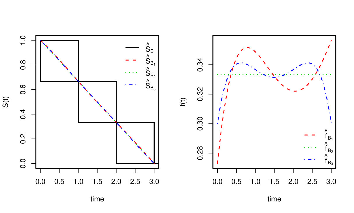 Figure 1
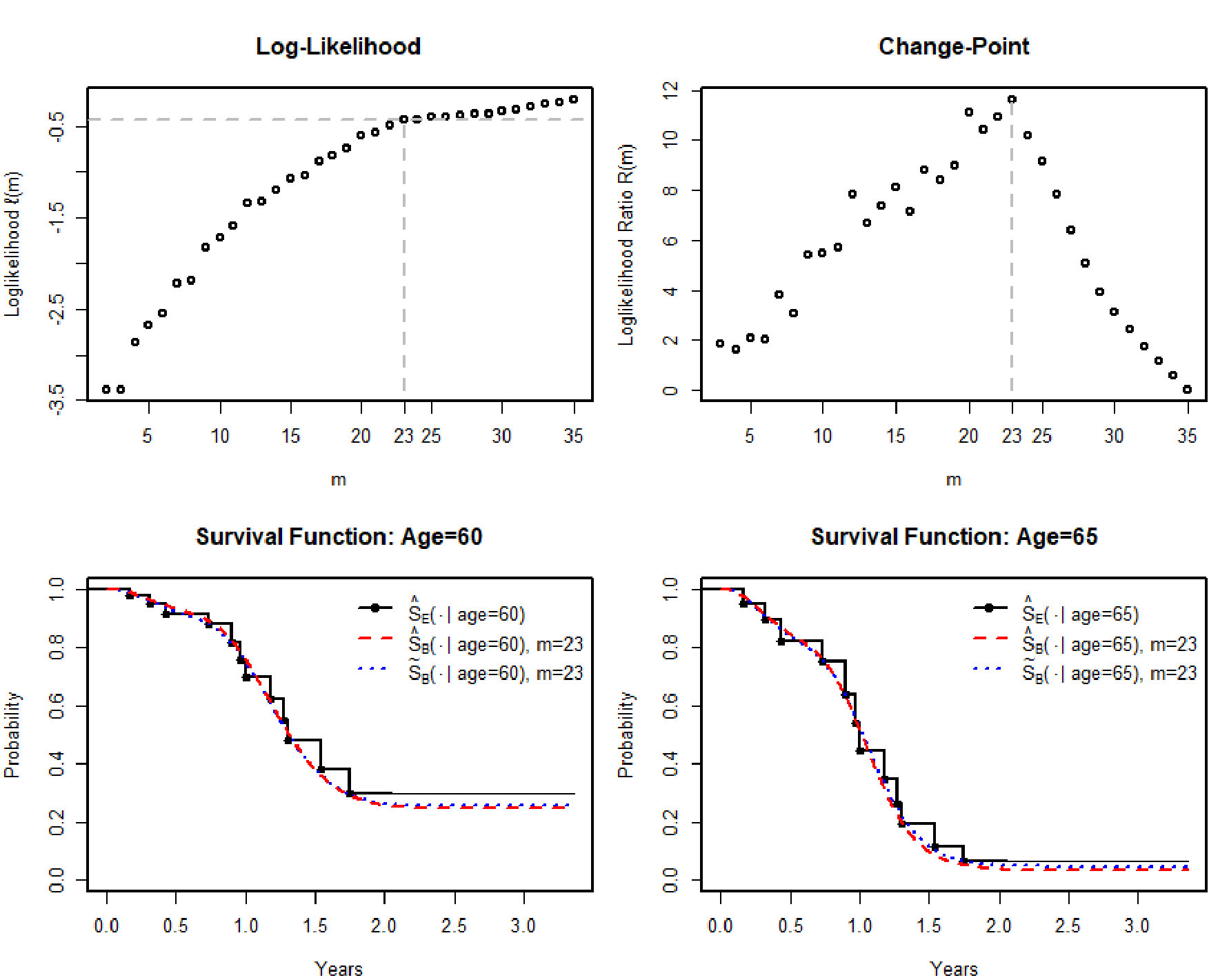 Figure 2
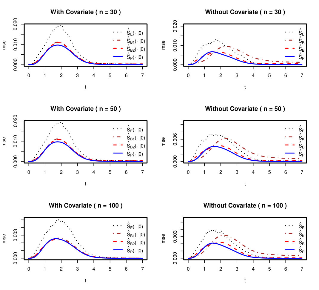 Figure 3
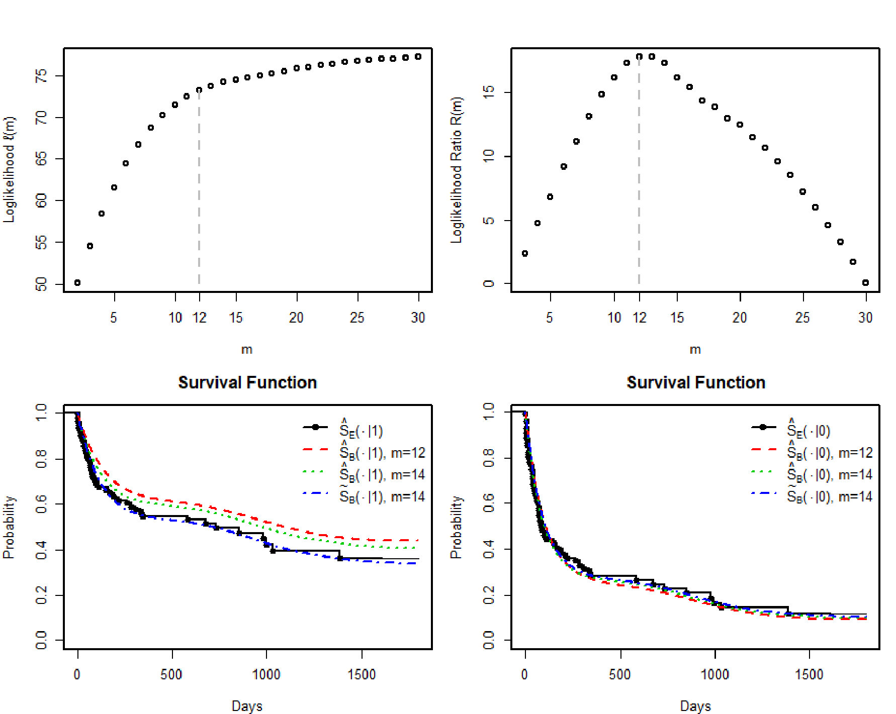 Figure 4