Low-cost ultrasonic distance measurement in a mechanical resonance experiment
William D. Joysey, Axel Mellinger

TL;DR
This paper introduces a low-cost ultrasonic sensor system for measuring mechanical resonance in lab courses, enabling students to efficiently collect data on amplitude and phase lag across frequencies.
Contribution
It presents a novel, affordable dual-probe ultrasonic measurement setup with real-time data processing suitable for educational settings.
Findings
Successful implementation of ultrasonic sensors for resonance measurement
Effective lag compensation using a modified Savitzky-Golay filter
Facilitates large-scale, hands-on physics experiments in educational labs
Abstract
We present a low-cost, dual-probe position sensor in a mechanical resonance experiment suitable for deployment in large lab courses with multiple stations. The motion of the two ends of a driven, damped spring oscillator is recorded with US-100 ultrasonic distance sensors and ESP8266 microcontrollers. Sensor lag is compensated via a modified Savitzky-Golay filter. Data is downloaded to a computer via Wi-Fi in a format suitable for analysis in Logger Pro. Due to the simple and fast data acquisition process, students can gather sufficient data to plot curves of the amplitude and phase lag as a function of driving frequency.
Click any figure to enlarge with its caption.
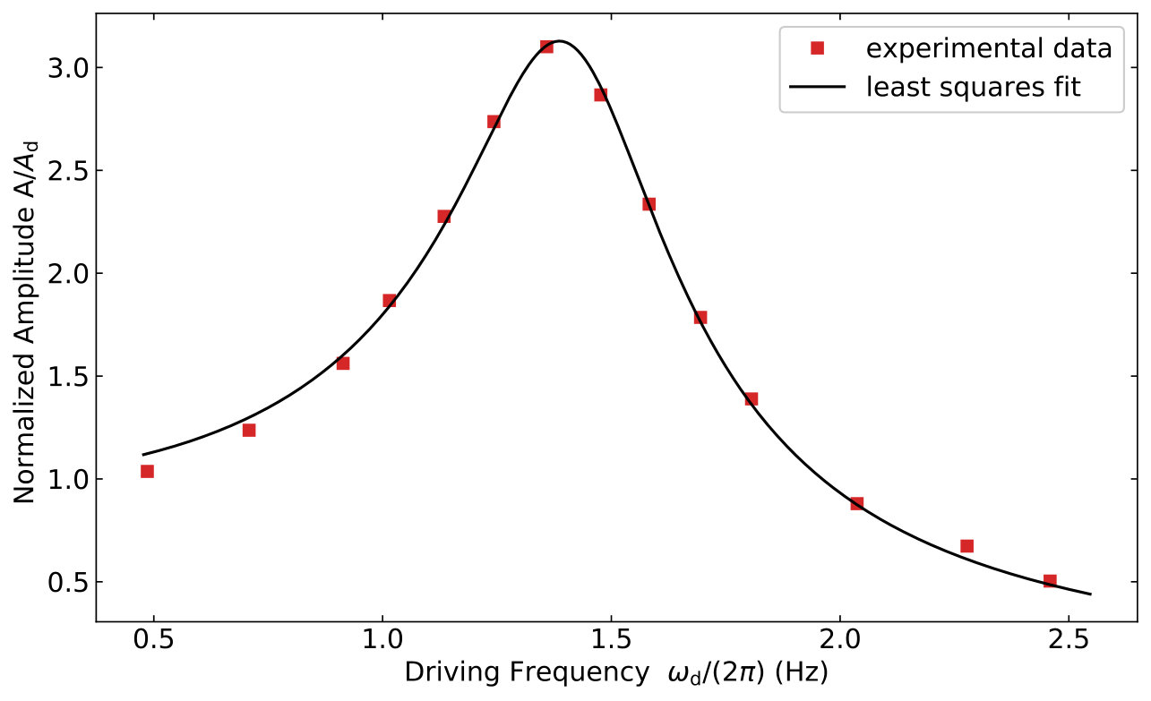 Figure 1
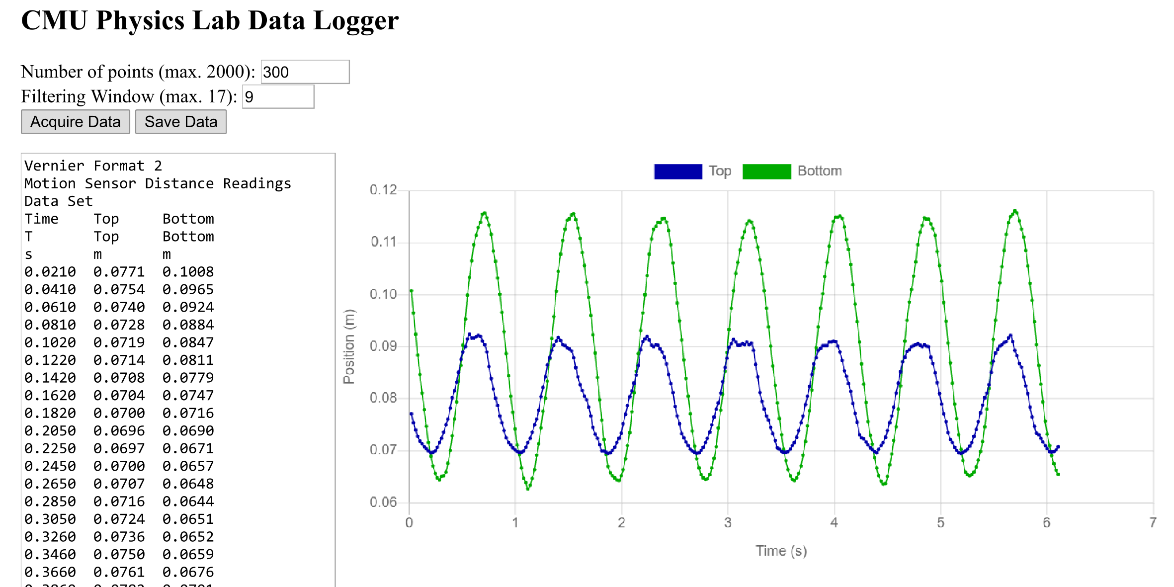 Figure 2
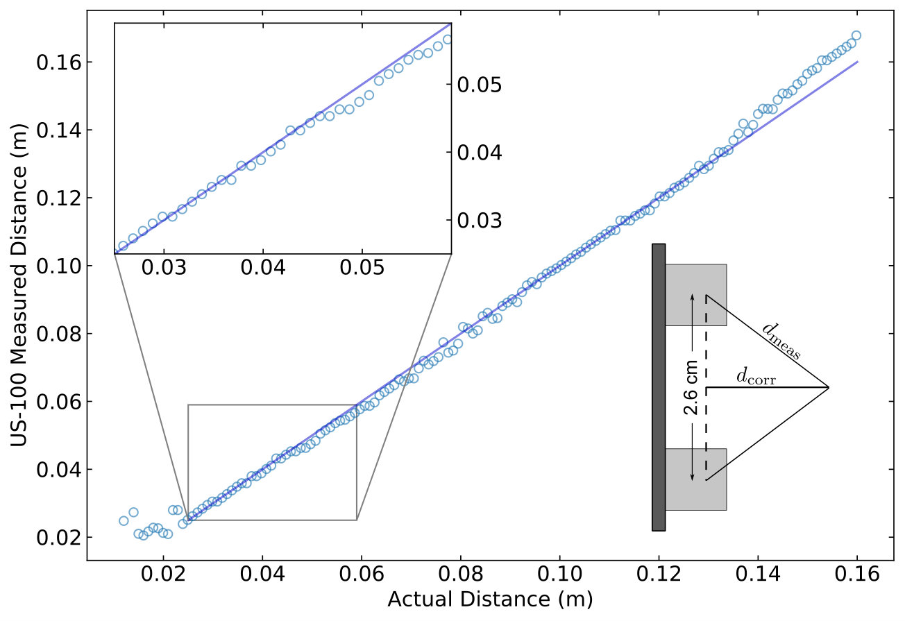 Figure 3
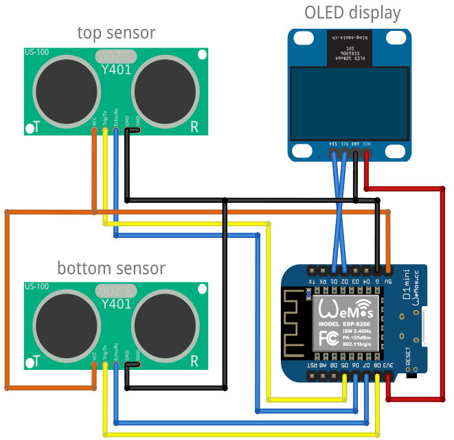 Figure 4
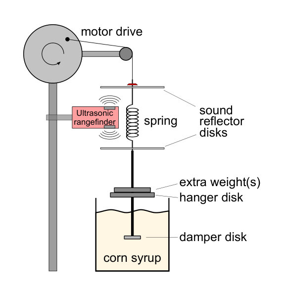 Figure 5
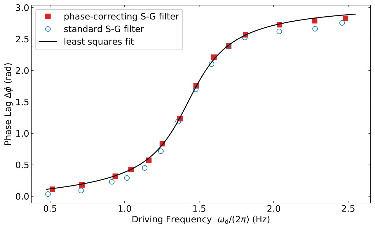 Figure 6
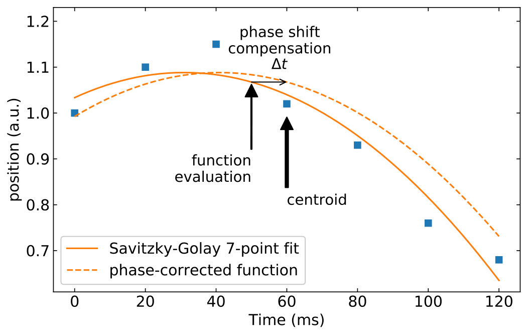 Figure 7
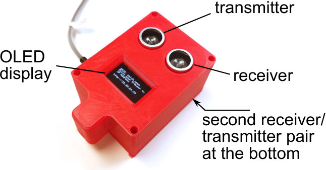 Figure 8
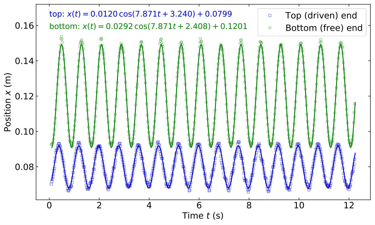 Figure 9
Peer Reviews
No public reviews on file for this paper yet. If you reviewed it on a platform where reviews are public (OpenReview, ICLR, NeurIPS, ICML), you can paste yours below so the community can read it here.
Code & Models
Videos
No videos yet. Explain this paper in a talk, walkthrough, or lecture? Add one.
Taxonomy
TopicsExperimental Learning in Engineering · Experimental and Theoretical Physics Studies · Sensor Technology and Measurement Systems
Low-cost ultrasonic distance measurement in a mechanical resonance experiment
William D. Joysey
Axel Mellinger
Department of Physics, Central Michigan University, Mount Pleasant, MI 48859
Abstract
We present a low-cost, dual-probe position sensor in a mechanical resonance experiment suitable for deployment in large lab courses with multiple stations. The motion of the two ends of a driven, damped spring oscillator is recorded with US-100 ultrasonic distance sensors and ESP8266 microcontrollers. Sensor lag is compensated via a modified Savitzky-Golay filter. Data is downloaded to a computer via Wi-Fi in a format suitable for analysis in Logger Pro®. Due to the simple and fast data acquisition process, students can gather sufficient data to plot curves of the amplitude and phase lag as a function of driving frequency.
I Introduction
Mechanical resonance is a key concept in physics and engineeringBauer and Westfall (2014), with many practical applications such as automotive vehicle suspensions and musical instruments. Resonance also occurs in electrical circuits, optics and at the atomic and nuclear scale. Therefore, studying driven, damped harmonic motion is a desirable experiment in many undergraduate physics lab courses. However, there appears to be a dearth of affordable, commercial equipment for such experiments. In some European countries, Pohl’s pendulum (a spring-loaded driven disk with electromagnetic induction damping) is a popular experiment in first-year lab coursesPohl (1944); PHYWE (2019), but it appears to be less common elsewhere. Moreover, the cost of such an apparatus is substantial, especially for large introductory physics lab courses with 10 or 20 identical stations. In this paper, we discuss a simple motor-driven coil spring oscillator (Fig. 1) with ultrasonic distance measurement.
The effect of mechanical resonance in a mass-spring oscillator is two-fold: (a) an increase in amplitude and (b) a phase lag between the free and driven ends of the spring oscillator. While the amplitude of a low-frequency oscillation can be measured with a simple ruler or meter stick, an accurate phase shift measurement requires that the positions of both the driven and free end of the spring be recorded as a function of time.
There is a variety of methods for measuring time-dependent positions in a physics lab experiment, including the venerable spark tapeOlson (1992), video analysisLaws et al. (2009), photogatesGaleriu (2013) and ultrasonic rangefindingGatland, Kahlscheuer, and Menkara (1992). In recent years, a number of compact, very low cost ultrasonic rangefinders have become popular in the maker community, and have also found use in physics labs to study simple harmonic Galeriu, Edwards, and Esper (2014); Goncalves, Cena, and Bozano (2017) and free-fallMoya (2018) motion. Their output can be recorded and processed with microcontrollers, such as the popular Arduino family,Bouquet et al. (2017); Lavelle (2018) or the Wi-Fi-enabled system-on-a-chip ESP8266 and ESP32 microcontrollers.Bensky (2018) Ultrasonic rangefinding is non-contacting (i. e. does not introduce extra friction), significantly less tedious than video analysis, has a resolution of and is robust enough to provide reliable data in a teaching lab.
II Theory
The theory of driven (forced) harmonic oscillators is covered by most introductory physics textbooksBauer and Westfall (2014). We assume a mass on a spring with spring constant , a damping force of (where is the velocity and is the damping parameter) and a periodic driving force . The differential equation of motion is
[TABLE]
with the steady-state solution
[TABLE]
where the amplitude is a function of the driving (angular) frequency :
[TABLE]
Here, is the natural angular frequency of the undamped oscillator. Due to inertia, the oscillation of mass lags the oscillation of the spring’s driven end by a phase angle
[TABLE]
With the experimental setup presented in this paper, both and can be measured.
III Apparatus
III.1 Mechanical Setup
A schematic view of the apparatus is shown in Fig. 1. A Pasco ME-8750 Mechanical Oscillator/Driver generates a low-frequency sinusoidal motion. A nylon thread connects the driver unit to a coil spring with a spring constant of approximately 20\text{,}\mathrm{N}\mathrm{/}\mathrm{m}. The bottom end of the spring is connect to a hanger with a 100 or $200\text{\,}\mathrm{g}$ mass and a damper disk ($25\text{\,}\mathrm{m}\mathrm{m}$ diameter) that oscillates in a beaker filled with corn syrup. The corn syrup was slightly diluted with water to obtain a damping constant of about $0.6\text{\,}\mathrm{k}\mathrm{g}\mathrm{/}\mathrm{s}$. The voltage applied to the motor ($012\text{\,}\mathrm{V}$) controls the oscillation frequency ($f_{\text{d}}\approx\,02.5\text{,}\mathrm{H}\mathrm{z}$).
The dual ultrasonic position sensor is mounted alongside the spring. It ultrasound pulses are reflected by two acrylic disks, mounted at the top and bottom end of the spring, respectively.
III.2 Electrical and Software Setup
Distances are measured by two US-100 ultrasonic rangefinders, widely available on Ebay and from robotic equipment vendors (cost approximately US $4 per item). Unlike the older (and slightly cheaper) HC-SR04 and US-015 sensorsGaleriu, Edwards, and Esper (2014), the US-100 can operate in two modes:
- •
the traditional trigger/echo mode, where a trigger signal of at least will cause the emission of a train of short ultrasound pulses. The sensor then generates a pulse on its echo pin, with a length equal to the ultrasound round-trip time.
- •
a serial communication protocol (9600 baud, 8 bits, no parity), where the distance measurement is initiated by sending a 0x55 character to the sensor’s trigger pin, and the distance to the object in mm is returned as a 2-byte integer on the echo pin.
For improved accuracy, the US-100 uses an on-board thermometer to calculate the speed of sound as a function of ambient temperature (serial mode only). Due to its compact size (approx. 40\text{\,}\mathrm{m}\mathrm{m}$\times$15\text{\,}\mathrm{m}\mathrm{m}) and its short minimum detection distance of , the US-100 rangefinder can be used in tight spaces.
In our setup, the rangefinders measure the distance to plastic disks attached to the top and bottom end of the spring (Fig. 1). Since they are located between the disks, the sign of the position reported by the top sensor needs to be inverted. In addition, an offset is applied, so that both positions are reported as positive values. The data from the distance sensors is collected using a WeMos D1 mini Wi-Fi microcontroller (cost approx. US 5).
The components are wired as shown in Fig. 2 and mounted in a 3D-printed enclosure (Fig. 3). Power is supplied via a micro-USB cable, either from the USB port of a computer, or a USB power supply. The ESP8266 software was written in C++ using the Arduino IDEArd (2019) and is available for download on Github.Mellinger (2019) The internal web server uses the jQuery and Chart.js JavaScript libraries.
When the unit is powered up, a greeting message is shown on the OLED display. The ESP8266 attempts to connect the university’s “open” (not password protected) Wi-Fi network. Should this network be unavailable, the ESP8266 switches to “soft access point” mode, setting up its own Wi-Fi network. Next, the a message similar to
SSID: cmich_open
Point your browser to IP Address http://aa.bb.cc.dd
is displayed. The student then navigates to the indicated URL using a web browser. Initially, a simple web form is shown (Fig. 4). The only user-defined input parameters are the number of data points to be recorded (10-2000), and the window width of the Savitzky-Golay (S-G) smoothing filter.Savitzky and Golay (1964)
A measurement is initiated by clicking the “Acquire Data” button. Upon completion, a graph of the positions (in meters) versus time (in seconds) is displayed. In addition, the data is returned as a 3-column ASCII table, which can be saved to the computer’s hard drive with the “Save Data” button. The table includes a few header lines to make the file recognizable by Vernier’s LoggerPro® software.Ver (2019)
IV Results and Discussion
IV.1 US-100 Linearity Test
To verify the accuracy of US-100 ultrasonic rangefinder it was mounted to a Zaber T-LSR 300B motorized linear slide and moved relative to a fixed target. Fig. 5 shows good linearity for distances from . At the sensor exhibits some non-monotonic behavior, which is a known property of low-cost ultrasonic rangefindersPilling (2019). Valid data is returned for distances as low as . At small distances the finite distance 2.6\text{,}\mathrm{c}\mathrm{m}$$ between transmitter and receiver has to be taken into accountGaleriu, Edwards, and Esper (2014), as shown in the inset of Fig. 5. Using the Pythagorean theorem, the corrected distance is .
IV.2 Driven Oscillator
IV.2.1 Amplitude
Fig. 6 shows a typical measurement result for a driving frequency slightly below resonance. The increase in amplitude at the bottom end of the spring is clearly visible, as is the phase lag.
Once the data has been imported into LoggerPro®, the students determine the amplitude and phase by fitting functions of the type
[TABLE]
to the top and bottom distances, where , , and are fit parameters. Sometimes, the fit fails and returns a nearly straight line (i. e. a cosine curve with a very small amplitude). In that case, students are encouraged to manually optimize the initial fit parameters before trying the automatic curve fit again.
From the least squares fit parameters of Eq. (5), the amplitude ratio of the free end over the driven end can be calculated and plotted as a function of frequency (Fig. 7). The results are in very good agreement with the curve of Eq. (3).
IV.2.2 Phase-shift correction
The two position measurements are taken approximately 10\text{,}\mathrm{m}\mathrm{s}$$ apart, due to the time required by the US-100 rangefinder to acquire and transmit a distance reading. At the shortest oscillator period (about ), this equals a phase difference of . While not a large amount, it becomes a noticeable artifact in a plot of phase lag versus frequency. It is, of course, possible to record separate time stamps for each rangefinder. However, handling two time columns introduces an additional workload for the students, and may prevent them from plotting both positions in a single graph.
Instead, we compensate this phase shift through a modification of the S-G filter. In the example shown in Fig. 8, a polynomial of order is fitted to a moving window of data points. Normally, this polynomial is evaluated at the centroid (here: 60\text{,}\mathrm{m}\mathrm{s}$$). To compensate the delay of the second (bottom) sensor, we instead evaluate the polynomial for the bottom data at a time earlier than the centroid. This is easily done using the first and second derivatives provided by the S-G filter:
[TABLE]
The phase shift correction is built into the ESP8266 code and is normally not revealed to students in introductory lab courses (although it could become a discussion point in an advanced physics lab). The S-G filter coefficients were calculated using the equations given by GorryGorry (1990), which correctly handle the first and last points in the data set, for which the filter kernel is non-symmetric (the number of points to the left and right differs). The effectiveness of the phase-shift correction can be seen in the phase lag plot of Fig. 9.
V Conclusion
We designed and built a dual-head ultrasonic position sensor for a driven oscillator experiment. The material cost for the sensor is under USx(t)A(\omega_{\text{d}})\Delta\phi(\omega_{\text{d}})$.
Compared to earlier uses of ultrasonic rangefinding in mechanical resonance experimentsGaleriu, Edwards, and Esper (2014); Goncalves, Cena, and Bozano (2017), the dual-head rangefinder allows the measurement of the phase lag. A modification to the Savitzky-Golay smoothing filter compensates for the delay introduced by sequentially reading out the rangefinders. This resulted in a noticeable improvement of the phase lag plot.
The ultrasonic rangefinder is suitable for use in a variety of other linear motion experiments, such as uniform and accelerated motion on low-friction air tracks. The sampling rate (50 samples/s for dual head recording, 100 samples/s when used with a single rangefinder) is fast enough to provide the students with a finely spaced data set.
Acknowledgements.
We gratefully acknowledge the help of Ray Clark and Mark Wilson in designing and building the resonance experiment and the sensor head. A.M. thanks Andrei Neacsu for many stimulating discussions on microcontrollers and sensors.
The reference list from the paper itself. Each links out to its DOI / PubMed record.
- 1Bauer and Westfall (2014) W. Bauer and G. D. Westfall, University Physics , 2nd ed. (Mc Graw-Hill, 2014) pp. 451–452.
- 2Pohl (1944) R. W. Pohl, Einführung in Mechanik, Akustik und Wärmelehre (in German) (Springer, 1944) p. 188.
- 3PHYWE (2019) PHYWE, “Forced oscillations – Pohl’s pendulum, https://www.phywe.com/en/forced-oscillations-pohl-s-pendulum.html ,” (retrieved June 2019).
- 4Olson (1992) J. Olson, The Physics Teacher 30 , 188 (1992) . · doi ↗
- 5Laws et al. (2009) P. W. Laws, R. B. Teese, M. C. Willis, and P. J. Cooney, Physics with Video Analysis (Vernier Software & Technology, Beaverton, OR, 2009).
- 6Galeriu (2013) C. Galeriu, The Physics Teacher 51 , 156 (2013) . · doi ↗
- 7Gatland, Kahlscheuer, and Menkara (1992) I. R. Gatland, R. Kahlscheuer, and H. Menkara, Am. J. Phys. 60 , 451 (1992) . · doi ↗
- 8Galeriu, Edwards, and Esper (2014) C. Galeriu, S. Edwards, and G. Esper, The Physics Teacher 52 , 157 (2014) . · doi ↗