Index Formulae for Line Bundle Cohomology on Complex Surfaces
Callum R. Brodie, Andrei Constantin, Rehan Deen, and Andre Lukas

TL;DR
This paper develops explicit index formulae for line bundle cohomology on complex surfaces, including del Pezzo, Hirzebruch, and toric surfaces, providing a unified approach and new theoretical insights.
Contribution
It introduces closed-form index expressions for line bundle cohomology on various complex surfaces and an algorithm to compute cohomology in terms of an index.
Findings
Derived explicit index formulae for del Pezzo and Hirzebruch surfaces.
Provided an algorithm for expressing cohomology of line bundles on toric surfaces.
Proved theorems relating effective and nef line bundles preserving cohomology.
Abstract
We conjecture and prove closed-form index expressions for the cohomology dimensions of line bundles on del Pezzo and Hirzebruch surfaces. Further, for all compact toric surfaces we provide a simple algorithm which allows expression of any line bundle cohomology in terms of an index. These formulae follow from general theorems we prove for a wider class of surfaces. In particular, we construct a map that takes any effective line bundle to a nef line bundle while preserving the zeroth cohomology dimension. For complex surfaces, these results explain the appearance of piecewise polynomial equations for cohomology and they are a first step towards understanding similar formulae recently obtained for Calabi-Yau three-folds.
Click any figure to enlarge with its caption.
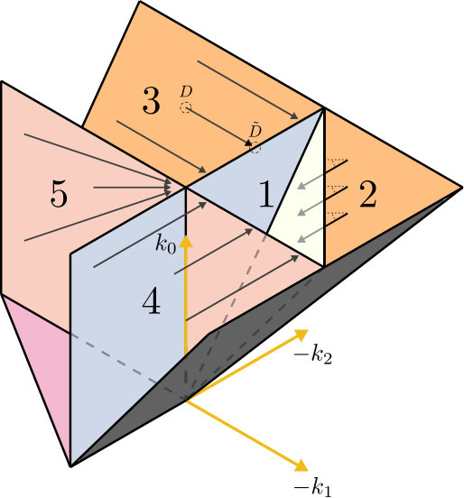 Figure 1
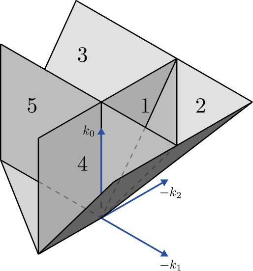 Figure 2
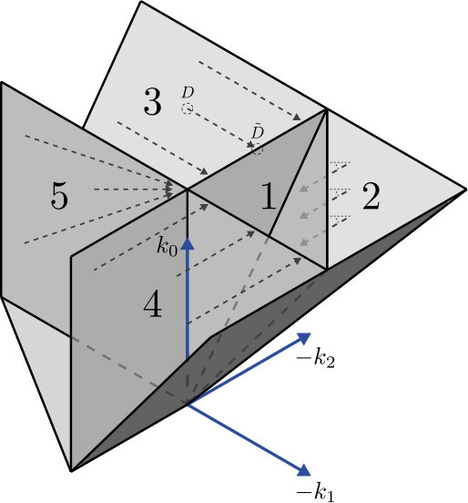 Figure 3
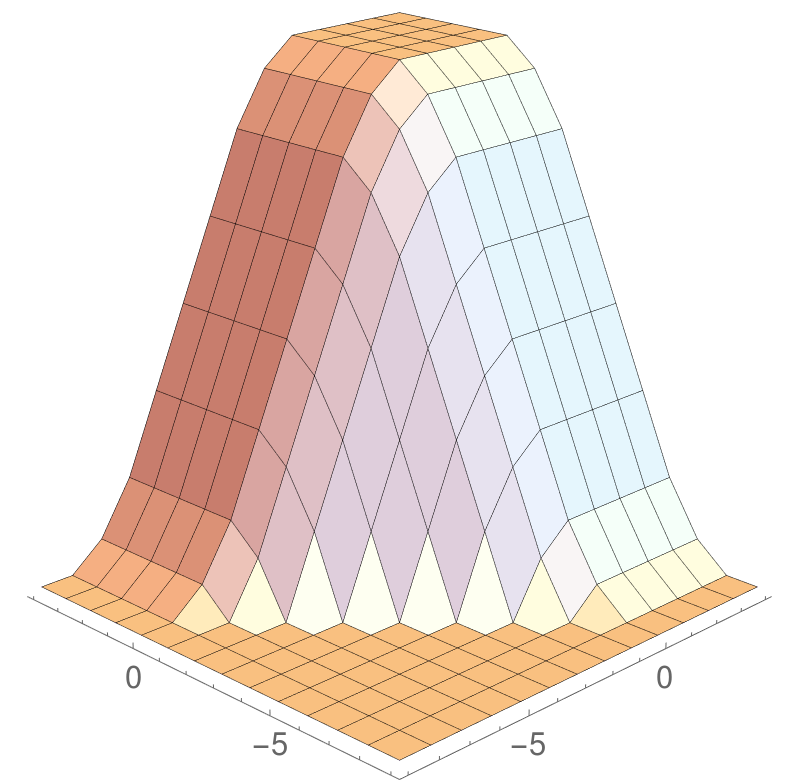 Figure 4
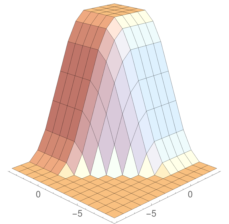 Figure 5
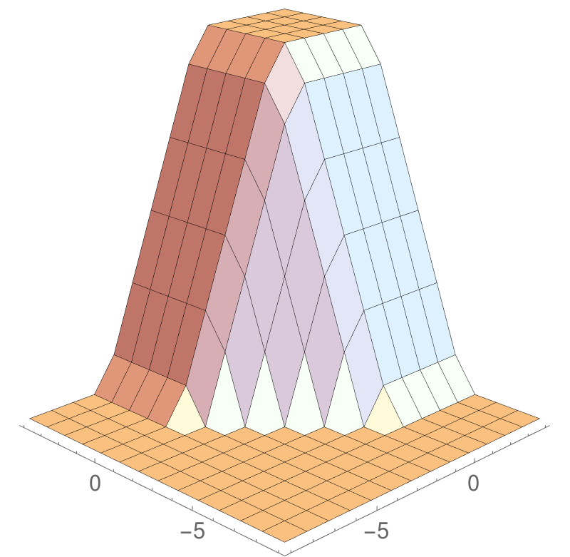 Figure 6
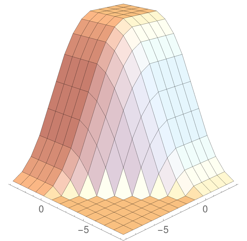 Figure 7
 Figure 8
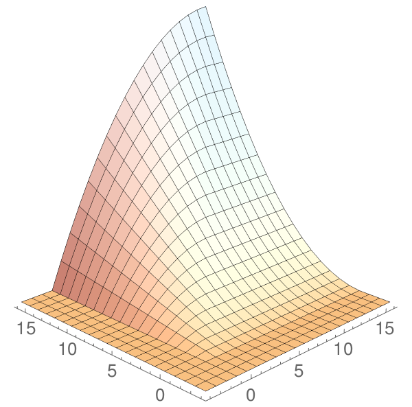 Figure 9
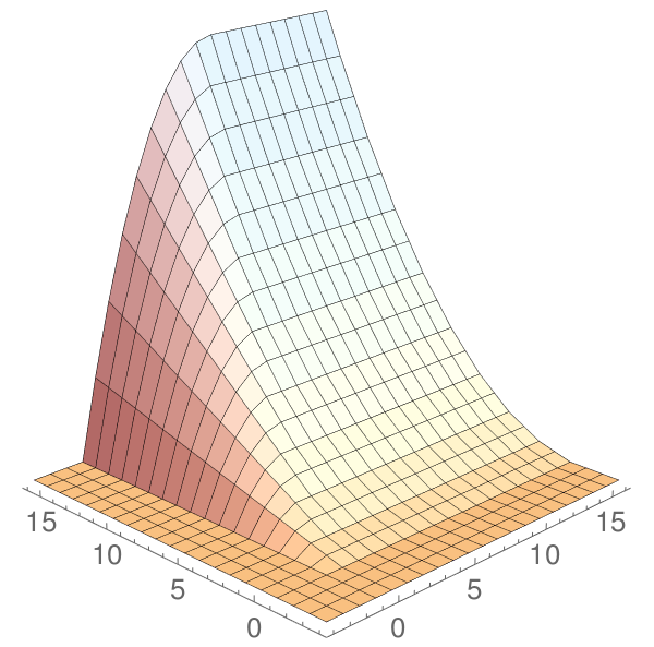 Figure 10
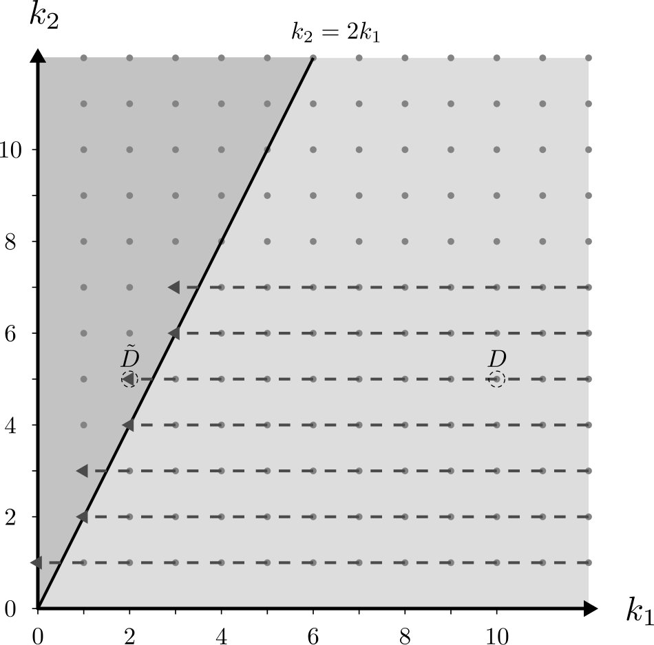 Figure 11
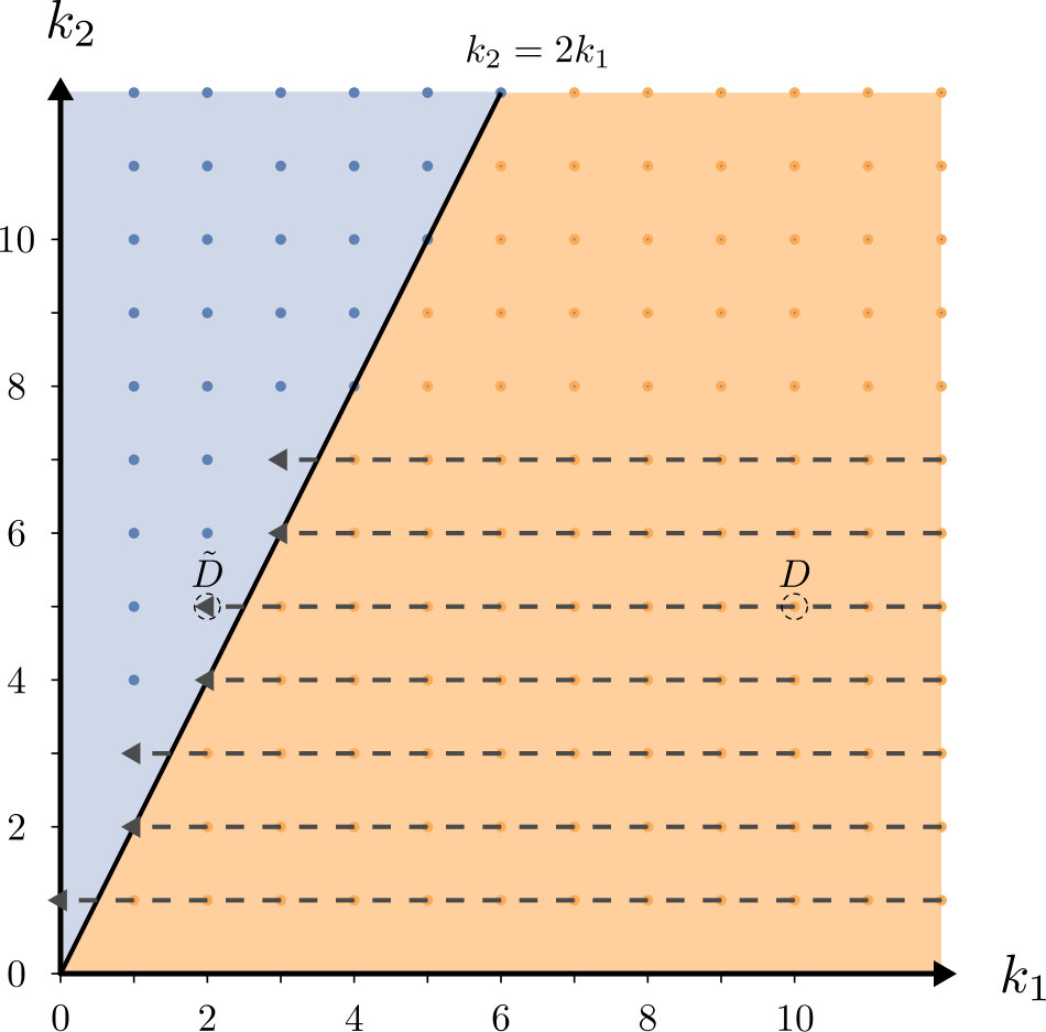 Figure 12
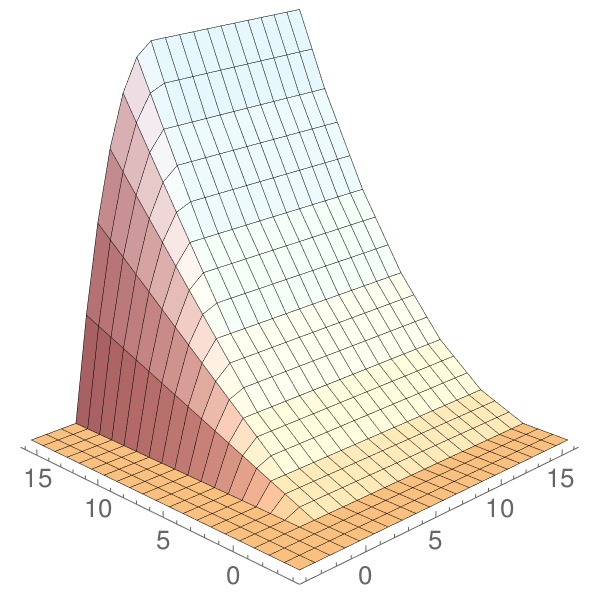 Figure 13
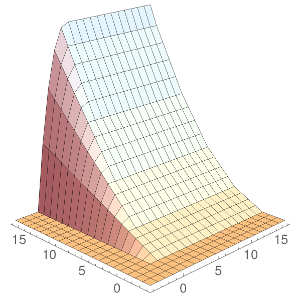 Figure 14
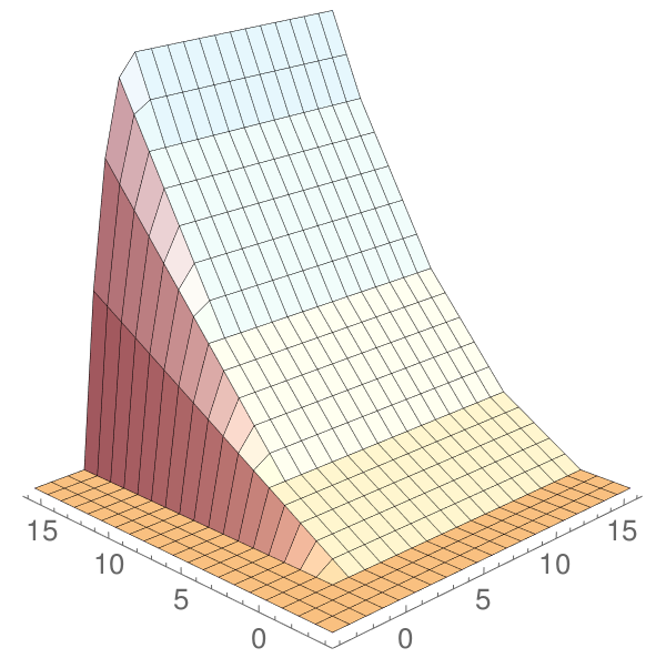 Figure 15
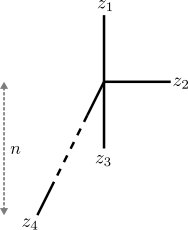 Figure 16
 Figure 17
Peer Reviews
No public reviews on file for this paper yet. If you reviewed it on a platform where reviews are public (OpenReview, ICLR, NeurIPS, ICML), you can paste yours below so the community can read it here.
Videos
No videos yet. Explain this paper in a talk, walkthrough, or lecture? Add one.
Index Formulae for Line Bundle Cohomology on Complex Surfaces
**Callum R. Brodiea,[email protected], Andrei Constantinb,[email protected], Rehan Deena,[email protected] , Andre Lukasa,[email protected],
a *Rudolf Peierls Centre for Theoretical Physics, University of Oxford,
Parks Road, Oxford OX1 3PU, UK *
b *Pembroke College, University of Oxford, OX1 1DW, UK
Mansfield College, University of Oxford, OX1 3TF, UK *
Abstract
We conjecture and prove closed-form index expressions for the cohomology dimensions of line bundles on del Pezzo and Hirzebruch surfaces. Further, for all compact toric surfaces we provide a simple algorithm which allows expression of any line bundle cohomology in terms of an index. These formulae follow from general theorems we prove for a wider class of surfaces. In particular, we construct a map that takes any effective line bundle to a nef line bundle while preserving the zeroth cohomology dimension. For complex surfaces, these results explain the appearance of piecewise polynomial equations for cohomology and they are a first step towards understanding similar formulae recently obtained for Calabi-Yau three-folds.
Contents
1 Introduction
Cohomologies of line bundles are crucial for various types of string compactifications, for example in the context of heterotic and F-theory model building. Usually, these cohomologies are computed using algorithmic methods, based on Čech cohomology, spectral sequences and related mathematical tools. These methods can be computationally intense and they provide little insight into the origin and structure of the results. This makes a bottom-up approach to string model building difficult whenever line bundles are involved. Clearly, string theory would profit from more direct and systematic access to line bundle cohomology and in this paper we report on some progress in this direction.
In Ref. [1] it was found that line bundle cohomology dimensions on (complete intersection) Calabi-Yau manifolds can be described by relatively simple formulae, which are piecewise polynomial.555The first non-trivial instance of a line bundle cohomology formula appeared in the earlier work [2, 3], in which generic hypersurfaces of type (2,2,2,2) in a product of four complex projective spaces were studied. More precisely, the Picard group of the manifold splits into a number of disjoint regions - which are frequently but not always cones - in each of which the cohomology dimensions are given by a cubic polynomial in the integers which label the line bundles. These results were obtained heuristically by looking at algorithmically computed cohomology data on a few complete intersection Calabi-Yau manifolds and smooth quotients thereof and by extracting analytic formulae from this data. The authors of Ref. [4] employed machine learning techniques to derive cohomology formulae for (hypersurfaces in) toric varieties. In a recent paper [5], these results were extended to a larger class of complete intersection manifolds with Picard number . The pattern conjectured from these results is that line bundle cohomology dimensions on manifolds with complex dimension are piecewise polynomial, with polynomials of degree (at most) . All this points to a yet to be fully discovered mathematical structure underlying line bundle cohomology.
In simple cases, it is possible to prove these results by spectral sequence chasing but this becomes tedious for more complicated manifolds. It is fair to say that the origin of these formulae for Calabi-Yau three-folds is currently not well-understood and that there is no simple and systematic method for their derivation. In fact, Calabi-Yau three-folds are fairly complicated objects and may not provide the best setting to uncover the structure underlying line bundle cohomology.
In the present paper, we, therefore, explore these issues in the simpler setting of complex surfaces. A line bundle over a complex surface has three cohomology dimensions , where , but knowledge of one of these for all line bundles implies the other two via Serre duality and the index theorem. For this reason, we will focus our study on the zeroth cohomology dimension, . Following standard notation, the line bundle associated to a divisor is denoted by and frequently we introduce a basis of divisor (classes), so that , with . Having fixed such a basis, we also occasionally write the corresponding line bundle as , where is an integer vector.
As a first step, we proceed in much the same way as was done for Calabi-Yau three-folds. We produce cohomology data from algorithmic methods and extract analytic formulae for the zeroth cohomology dimension by “eyeballing”. The examples we will be studying in this context are the Hirzebruch and del Pezzo surfaces. The results turn out to be as expected and are analogous to the ones obtained for Calabi-Yau three-folds. The dimensions are described by equations which are piecewise quadratic in the integers . This provides further evidence that piecewise polynomial formulae for line bundle cohomology dimensions are a general feature which is neither limited to the Calabi-Yau case nor to three complex dimensions.
However, for surfaces we are able to go further. For both Hirzebruch and del Pezzo surfaces we are able to express the piecewise quadratic formulae in terms of basis-independent, intrinsic objects, specifically the generators of the effective and nef cones, the irreducible negative self-intersection divisors and the intersection form on . This re-writing suggests a specific map for effective divisors which we provide explicitly and which leaves the zeroth cohomology dimension unchanged, that is, . We further observe that for all Hirzebruch and del Pezzo surfaces the line bundle satisfies for . Combining these statements implies that the cohomology of can be computed in terms of the index of the shifted divisor as
[TABLE]
At this stage, the result (1.1) for Hirzebruch and del Pezzo surfaces together with the map is still empirical, that is, inferred from a finite set of cohomology data.
Based on these empirical results, we write down a general form of the map which applies to all smooth compact complex projective surfaces and we prove that it preserves the zeroth cohomology dimensions, that is, . Moreover, it follows that iterating the map leads, after a finite number of steps, to a divisor in the nef cone. Provided there is a vanishing theorem which asserts that for , it follows that
[TABLE]
For such cases, which we show include Hirzebruch and del Pezzo surfaces as well as all compact toric surfaces we have, therefore, a mathematical proof for the existence of index formulae for and a practical way of deriving them. These formulae are quasi-topological in nature: the quantity )) is purely topological, while the map depends in general on the complex structure.
For Hirzebruch and del Pezzo surfaces we prove that a single application of the map already projects into the nef cone and that a suitable vanishing theorem is available in either case. This leads to a mathematical proof for the empirical formula (1.1).
We will presently provide a summary of our main results. Subsequently, the plan for the remainder of the paper is as follows. In the next section, we explain how cohomology formulae can be extracted from cohomology data, computed by algorithmic methods, focusing on Hirzebruch and del Pezzo surfaces. In a first instance, we extract piecewise quadratic formulae from the data which are subsequently refined to index formulae. The reader less interested in this “empirical” aspect of the work can skip to Section 3 which contains our main mathematical statements. Section 4 illustrates these mathematical results in the context of simple examples. We conclude in Section 5.
The present paper has two companion papers. In Ref. [6], we explore how techniques from machine learning can help to uncover the structure of line bundle cohomology. Ref. [7] is more mathematical in style and provides rigorous proofs for the various mathematical statements presented here.
Summary of results
We outline below the way in which the index formulae can be applied to specific surfaces. For a smooth compact complex projective surface we first require knowledge of the effective (Mori) cone666For the examples discussed in this paper the Mori and the effective cones coincide, though there exist surfaces for which this is not the case, see e.g. Example 1.5.1 in Ref. [8]., . In practice this amounts to providing the set of Mori cone generators or the set of generators of the nef cone , which is dual to the Mori cone. We also need to know the intersection form on . For all divisors not in the Mori cone, that is , we have . On the other hand, all divisors have strictly positive zeroth cohomology dimension. For such effective divisors we define the map by
[TABLE]
where the sum runs over the set of all irreducible curves with negative self-intersection. The Heaviside function ensures that only curves with contribute to the sum and is the ceiling function. Hence, to write down this map explicitly, we need to know the irreducible, negative self-intersection curves on the surface - information that can be obtained for many cases of interest.
The key statement about the map (1.3) is that it leaves the zeroth cohomology dimension unchanged, that is, . Since the nef cone is the cone of divisors which intersect all algebraic curves non-negatively, it is clear that repeated application of the map (1.3) eventually leads to a divisor in the nef cone. If there is a vanishing theorem, typically Kodaira vanishing or one of its refinements, which asserts that for then the zeroth cohomology can be written as an index, using Eq. (1.2). It turns out that this is the case for many surfaces of interest, including Hirzebruch surfaces, del Pezzo surfaces, and compact toric surfaces, and, hence, index formulae for the zeroth cohomology dimensions exist for all these cases. The relevant vanishing theorems will be reviewed in the main text.
Let us first summarise how this general result applies to Hirzebruch surfaces . The Picard lattice of all Hirzebruch surfaces is two-dimensional and we can introduce a basis of divisor classes, such that the intersection form is defined by , and (see Appendix A for details). Then, the Mori cone is generated by and . This means effective divisors are of the form with non-negative and all other divisors with at least one negative have vanishing zeroth cohomology. The unique irreducible class with negative self-intersection is . Inserting all this into the map (1.3) shows that is already in the nef cone. Theorem 3.3 guarantees the necessary vanishing, so that Eq. (1.1) can be applied. Combining these results we obtain the index formula
[TABLE]
for the zeroth cohomology dimension of effective divisors on Hirzebruch surfaces. The explicit formula for the index of line bundles on Hirzebruch surfaces is provided in Eq. (2.7).
Let us now summarise the analogous results for del Pezzo surfaces. Del Pezzo surfaces (other than which is trivial in our context) are blow-ups of the projective plane in generic points, where , and they are denoted by . The rank of their Picard lattice is and a standard basis of divisor classes consists of the hyperplane class of and the classes of the exceptional divisors associated to the blow-ups, where . The intersection form is fixed by the relation , and . The list of generators of the Mori and nef cones is too long, at least for the larger values of , to be listed here but has been explicitly provided in Appendix B. The irreducible negative self-intersection classes are precisely the Mori cone generators, which have self-intersection . It can be shown that a single application of the map (1.3) projects into the nef cone and Corollary 3.4 provides the appropriate vanishing statement so that Eq. (1.1) holds. This leads to the index formula
[TABLE]
for the zeroth cohomology dimension of effective divisors on del Pezzo surfaces, where are the generators of the Mori cone.
2 From data to index formulae
The mathematical results presented in this paper have been motivated following a somewhat unorthodox method which might be described as experimental algebraic geometry. The starting point is line bundle cohomology data on various surfaces, produced by algorithmic methods. From this data, we first read off simple piecewise quadratic formulae for cohomology dimensions. These formulae are then put through a process of gradual refinement until they are expressed in terms of intrinsic geometric objects of the underlying surface. In this form, the equations are very suggestive and lead to conjectures for line bundle cohomology on smooth compact complex projective surfaces which we state and prove in the next section. The main purpose of the present section is to describe this “experimental” approach, focusing on our two main classes of examples, the Hirzebruch and del Pezzo surfaces. This may be of interest to anyone wishing to pursue a similar procedure, for example for a different class of manifolds. The reader mainly interested in the general mathematical results for surfaces can safely skip this section and move on to Section 3.
2.1 Outline of approach
We have already mentioned Refs. [1, 5], where piecewise cubic formulae for line bundle cohomology dimensions on certain Calabi-Yau three-folds have been obtained, starting with cohomology data computed by algorithmic methods. These results suggest that line bundle cohomology dimensions on surfaces, , can be described by formulae which are piecewise quadratic in the integers which label the line bundles. This expectation, which we will confirm for our examples, as well as for larger classes of surfaces, is the starting point of our discussion. We will then gradually refine the piecewise quadratic equations in and attempt to re-write them in terms of intrinsic geometric objects, in our quest to uncover the mathematical origin of these equations.
Let us first recall that line bundles on surfaces have three cohomology dimensions, , where . However, Serre duality and the index theorem provide two relations
[TABLE]
between those three quantities. Here, is the canonical bundle777We will freely write the same symbol for the canonical divisor. It will be clear from context which is in use. of the surface and the index, , of the line bundle can be easily computed from the Riemann-Roch formula as
[TABLE]
where is the Euler characteristic. Written in terms of the line bundle integers the index is a quadratic polynomial. The upshot of this discussion is that knowledge of all zeroth cohomology dimensions for all line bundles determines all other cohomology dimensions. Moreover, piecewise quadratic formulae for directly translate into piecewise quadratic formulae for and via the above relations. For this reason, we will focus on the zeroth cohomology dimension in the following.
The basic steps of our approach are as follows.
- •
For the complex surface , we generate cohomology data, , for a range of integer vectors , typically taken from a box with , computed using suitable algorithmic methods.
- •
From this data, we extract conjectures for piecewise quadratic formulae for as a function of . Typically this is done by first identifying the regions in the Picard lattice for which the behaviour is quadratic. The experience from Calabi-Yau three folds suggests that these regions are frequently - but not always - cones. For each such region, we then fit a quadratic polynomial in to the data. In a companion paper [6] we explain how this process can be facilitated by methods from machine learning.
- •
Next, we attempt to re-write the piecewise quadratic formulae in in a basis-independent way, using intrinsic geometric objects of the underlying surface. For the surfaces we treat, one finds that the relevant objects are the effective (Mori) cone and its list of generators , the nef cone and its list of generators , the irreducible negative self-intersection curves and the intersection form on .
- •
Finally, we would like to bring the formula into a compact, manageable form. This is particularly relevant for surfaces with high Picard number, where the number of regions in the Picard lattice and, hence, the number of case distinctions required can be large. It turns out that such a compact form can indeed be found using the formula for the index. In this final form, our empirical results are quite suggestive and point to more general mathematical statements which we formulate and prove in Section 3.
The above programme will be carried out for two main classes of surfaces, the Hirzebruch and del Pezzo surfaces, and we now briefly review their basic properties.
2.2 Basic properties of Hirzebruch surfaces
The Hirzebruch surfaces are indexed by a non-negative integer . They correspond to different fibrations of a fibre over a base, with characterising the twisting. Their non-zero Hodge numbers are and and, hence, the Picard number is two for any . The Picard lattice is spanned by the classes of the two projective lines that form the fibre bundle. There exist toric and complete intersection representations of the Hirzebruch surfaces, and details of these have been relegated to Appendix A. Here, we focus on a few basic properties, relevant to our discussion, which can, for example, be deduced from the toric description. We write for the divisor888For most of the paper, the term “divisor” is used as a short-hand for “divisor class”. Whenever the distinction between divisor and divisor class becomes relevant we will state this explicitly. corresponding to the base of the fibre bundle, and for the divisor corresponding to the fibre. Then, the intersection form of is determined by
[TABLE]
Divisors on can be written as linear combinations with and line bundles are parametrised by two-dimensional integer vectors .
The two divisors and also correspond to the generators of the Mori cone , that is,
[TABLE]
This means effective divisors are of the form with . In addition, from the above intersection form, the dual nef cone has generators
[TABLE]
The anti-canonical divisor of the Hirzebruch surface is given by
[TABLE]
Inserting into the Riemann-Roch formula (2.2) an arbitrary divisor , the above expression for the anti-canonical divisor and the result (which follows from the second equation (2.2) with and ) gives
[TABLE]
There are several algorithmic methods to compute line bundle cohomology on Hirzebruch surfaces.
- •
Using the toric realisation of the Hirzebruch surfaces (see Appendix A), the dimension of the zeroth cohomology, which is all we require for our discussion, can be computed from the weight system.
- •
Hirzebruch surfaces can also be constructed as complete intersections in products of projective spaces (see Appendix A) and the techniques described in Refs. [9, 10, 11, 12, 13], based on the Bott-Borel-Weil formalism and spectral sequences, can be applied.
- •
Finally, again using the toric realisation, we can use the methods to calculate line bundle cohomology on toric spaces developed in Refs. [14, 15, 16].
2.3 Basic properties of del Pezzo surfaces
A del Pezzo surface is isomorphic to either or to a blow-up of the complex projective plane in generic points. The cases of and are trivial for our purposes since the result directly follows from Bott’s formula for line bundle cohomology on projective spaces. For this reason we focus on del Pezzo surfaces which correspond to a blow-up of in generic points, and we denote these surfaces by .
Del Pezzo surfaces can be realised as complete intersections in products of projective spaces and, for , as toric spaces. Details of this are provided in Appendix B. Here, we merely collect the information essential to our discussion.
The non-zero Hodge numbers of del Pezzo surfaces are and , so the rank of the Picard lattice is . A basis for the Picard lattice is given by , where is the hyperplane class of and , where , are the exceptional classes, related to the blow-ups. Relative to this basis, the intersection form is defined by the relations
[TABLE]
A general divisor is written as
[TABLE]
with and, hence, line bundles are labelled by -dimensional integer vectors . For another divisor with components the intersection form can also be written as
[TABLE]
The lists of Mori and nef cone generators are denoted by and respectively, and they are thought of as containing the actual divisors or their coordinates vectors relative to the basis , depending on context. In the latter form, they are explicitly provided in Appendix B.
The anti-canonical class of is given by
[TABLE]
Inserting into the Riemann-Roch formula a general divisor (2.9), the above expression for the anti-canonical class and the result (which follows from the second Eq. (2.2) with and ) gives
[TABLE]
As for Hirzebruch surfaces, there are several algorithmic methods available to calculate line bundle cohomology on del Pezzo surfaces.
- •
For the del Pezzo surfaces , with which have a toric realisation (see Appendix B), we can compute either from the toric weight system or via the methods for line bundle cohomology on toric spaces from Refs. [14, 15, 16].
- •
All del Pezzo surfaces have a realisation as complete intersections in products of projective spaces (see Appendix B), so the methods of Refs. [9, 10, 11, 12, 13] can be applied.
- •
It was noticed in Appendix B of Ref. [17] that line bundle cohomology on del Pezzo surfaces can be computed by counting certain polynomials on and we use a computational implementation of this method.
There is one further result which relates line bundle cohomology of del Pezzo surfaces for different which will be helpful in the following. The cohomology dimension of a divisor on with no component along the exceptional class is the same as the cohomology dimension of seen as a divisor on , that is,
[TABLE]
This can be shown, for example, by thinking about blowing-down one exceptional divisor or by using the relation between del Pezzo cohomology and polynomials on from Ref. [17].
2.4 Warm up: line bundle cohomology on Hirzebruch surfaces
The complexity of our task clearly increases with the Picard number of the surface. Hirzebruch surfaces, which all have Picard number two, therefore provide a simple setting for an initial exploration. In particular, it is possible to plot cohomology data and identify the regions in the Picard lattice by “eyeballing”. Once the regions are known, the quadratic polynomials can be fixed by a simple fit to a number of points in each region. This results in a piecewise quadratic formula which represents the first step on our path from data to general mathematical statements. Of course this piecewise quadratic formula should then be checked against all available cohomology data.
We recall that line bundles on Hirzebruch surfaces are labelled by a two-dimensional integer vector , relative to the divisor basis introduced in Section 2.2. In Figure 1 we plot the zeroth cohomology dimension, , as a function of , for the first three Hirzebruch surfaces , and . For a better visualisation, we have joined the discrete data points into a surface.
We recall from Section 2.2 that the cone of effective divisors, that is, the region where , is characterised by and . This is consistent with the plots in Figure 1 which indicate a non-zero cohomology precisely in the positive quadrant.
What is the structure in the positive quadrant? The obvious feature in the plots for and in Figure 1 is the presence of two regions which we expect require two different quadratic polynomials. In fact, it can be checked that this structure persists for all Hirzebruch surfaces with and that the two regions are separated by the hyperplane through the origin, described by the equation
[TABLE]
Now that we have identified the regions we can attempt polynomial fits. The region corresponds to the easy case. Here, the relevant polynomial for all Hirzebruch surfaces is simply the index, given in Eq. (2.7). The other region, where and which exists for all Hirzebruch surfaces with , is more problematic. A polynomial fit to the data in this region succeeds for but it fails for and all higher Hirzebruch surfaces. The problem becomes apparent when we plot the cohomology data for , , and as we have done in Figure 2.
The cohomology values in the region show a mod structure which can of course not be captured by a single quadratic polynomial. A similar structure has been observed in some of the examples studied in Ref. [4]. However, it is not too difficult to account for this mod behaviour by including a ceiling function. This leads to the following conjecture
[TABLE]
for the zeroth cohomology dimension on any Hirzebruch surface . The explicit expression for the index can be found in Eq. (2.7). This result lends further support to the conjecture that line bundle cohomology on complex surfaces is described by equations which are (basically) piecewise quadratic. However, the appearance of the ceiling function which accounts for the mod behaviour is new and, as we will see, points to an important feature of the more general formula we are seeking.
This completes the first two parts of our programme. The remaining tasks are, firstly, to write Eq. (2.15) in a basis-independent way and, secondly, to find a compact form, in terms of natural geometric objects. The current example of the Hirzebruch surfaces is simple enough to carry out both steps at once.
Consider first the boundary between Region 1 and Region 2. A quick glance at the intersection rules (2.3) shows that, for , we have . Hence, these two regions can be characterised by saying that needs to be in the effective cone, while, in addition, we require that for Region 1 and for Region 2. Finally, Region 3 is characterised by saying that is not in the effective cone. Since we can think of as the unique irreducible divisor with negative self-intersection, this provides a natural basis-independent formulation of the regions.
What about the polynomial expressions in those regions? In Region 1, the cohomology is already described by an intrinsic geometrical object, the index, but it is not immediately obvious how to proceed in Region 2. A useful observation is that the cohomology dimension in Region 2 does not depend on . This means that a projection exists: one can relate a cohomology result in Region 2 to one in Region 1 by a lattice projection along the negative direction. Since cohomology dimensions in Region 1 are described by the index we conclude that the same must be true for Region 2, however, the argument of the index is now a different, projected divisor. It turns out that the required lattice projection is
[TABLE]
with . Note that the expression on the right-hand-side is written entirely in terms of natural geometric objects of the Hirzebruch surface. With this projection, we can re-write the cohomology Eq. (2.15) as
[TABLE]
where is the unique irreducible divisor with negative self-intersection and is the Heaviside step function, defined by for and otherwise.
The above result, albeit in a very suggestive mathematical form, is still a conjecture since it has been extracted from a finite amount of cohomology data. In fact, Hirzebruch surfaces are sufficiently simple so that a direct proof can be found, for example from the weight system of the associated toric diagrams. We will not pursue this explicitly since, as we will see, Eq. (2.17) will direct us towards the general mathematical results in Section 3, of which it will turn out to be a special case.
2.5 Regions and polynomials for del Pezzo surfaces
We would now like to repeat the process from data to a concise mathematical formula for the case of del Pezzo surfaces. This is of course considerably more complicated, given that Picard numbers reach up to nine. In fact, writing down piecewise polynomial formulae explicitly becomes impractical for higher Picard numbers as the number of regions and, hence, case distinctions required, increases considerably. This is of course one of the reasons we are seeking concise mathematical formulae for cohomology dimensions.
We will tackle the problem of finding concise formulae in the next two sub-sections, but presently we would like to explain how to extract piecewise polynomial formulae from data. In practice we begin with the lower del Pezzo surfaces, , and gradually increase . Eq. (2.13) tell us that the structure found for is preserved as we move on to . This means that at each stage we have some partial information available from the del Pezzo surfaces with lower . For example, when determining some hyperplane boundaries, we already know some entries in their normal vectors.
The first step is to find the region boundaries and regions. Once this has been accomplished it is easy to find the quadratic polynomial in each region by a simple fit to the data. For the cases and we can proceed as for the Hirzebruch surfaces, that is, by simply reading the boundaries off from a plot. Even for higher Picard numbers it is possible to proceed by “eyeballing” if we focus on two-dimensional slices in the Picard lattice and combine the information from various such slices. We recall that line bundles on are labelled by an -dimensional integer vector , with the associated divisor given in Eq. (2.9).
Let us illustrate the process of finding the region boundaries for the example . The Picard number of this space is five, so a two-dimensional slice misses the behaviour of a boundary in the remaining three directions. We begin with slices in the plane, taken for various fixed choices of the remaining coefficients . In Figure 3 we have plotted four such two-dimensional slices through the Picard lattice of which show several region boundaries. As an example, we focus on the diagonal boundary which separates the regions of zero and non-zero cohomology.
The dependence on and is immediately clear: this boundary must be of the form . To find the dependence on the remaining , we compare slices. Take as a starting point the slice with (upper left plot). When we increase (upper right plot), the boundary advances by one unit and when decreases by one (lower left plot), the boundary recedes by one unit. Finally, when we instead increase (lower right plot), the boundary advances by two units. Hence the equation of this boundary is
[TABLE]
As one would expect, four slices were sufficient to determine this boundary. The other boundaries visible in Fig. 3 can be determined in the same way. The polynomials can then be obtained by a fit to the data in each region. The formulae obtained in this way are of course still conjectures, extracted from a finite amount of cohomology data.
As already mentioned, the piecewise polynomial formulae for become quite complicated for larger and have too many case distinctions to be reproduced here. However, it is possible to discuss in a concise way and we do this now for illustration. The Picard number of this surface is three and line bundles are labelled by a three-dimensional integer vector . Figure 4 is a plot of the regions that correspond to distinct polynomials. All region boundaries in this case are hyperplanes through the origin, so the regions themselves are cones with their bases at the origin.
Evidently, there are five distinct non-zero regions as numbered in the diagram, and they are described by the following sets of inequalities.
[TABLE]
Note that Region 1 is the nef cone and that the union of the five regions is the Mori cone. The polynomials that describe the zeroth cohomology dimension in each of these five regions are as follows.
[TABLE]
The main features of this formula - regions which are cones with bases at the origin and cohomology dimensions described by a quadric in each region - persist for all del Pezzo surfaces. Writing down the analogous formulae for with becomes impractical as the number of regions increases very quickly with . For this reason, we will now extract a more concise formula which works for all del Pezzo surfaces.
There is a more sophisticated way to extract regions and polynomials from data by using methods from machine learning. This will be discussed in detail in a companion paper [6].
2.6 A compact formula for del Pezzo surfaces
The first step towards extracting a concise formula which works for all del Pezzo surfaces is to understand the structure of the hyperplanes which separate the regions. Each such hyperplane is determined by a normal vector such that the boundary is described by the equation , where is the intersection matrix in Eq. (2.10). For these normal vectors can be read off from the inequalitites in the first three columns of (2.19), while the last three columns correspond to the boundaries of the Mori cone. Repeating the exercise for we find the following lists of normal vectors.
[TABLE]
For , the normal vectors have the same structure as for but with the other obvious permutations included. The same is true for , except, additionally, the new vector appears.
The reader familiar with the properties of del Pezzo surfaces will immediately recognise the above divisors as the generators of the Mori cone or, equivalently, as the exceptional divisors with self-intersection . We conclude that the bounding hyperplanes for the various regions are described by the Mori cone generators and, it turns out, this holds for all with . We denote the set of Mori and nef cone generators for by and , respectively, and their elements are explicitly listed in Appendix B.
Our next task is to find the quadratic polynomials that describe the cohomology in the various regions of the Picard lattice. To this end, it is instructive to look at the difference between two polynomials and in neighbouring regions, separated by a boundary hyperplane with normal vector . By inspecting examples, it turns out that the change is always of the form
[TABLE]
where is a linear expression in the with integer coefficients. In fact these integer coefficients follow a pattern too. If the region with polynomial is characterised by and the one with polynomial by , where , then we have
[TABLE]
The above term on the right-hand side appears when we cross a boundary with normal vector into a region with . It is therefore natural to start in the “simplest” region where for all . This region is of course precisely the nef cone , the dual of the Mori cone, where the zeroth cohomology dimension is given by the index. Hence, for the divisor , we have the following formula
[TABLE]
for the zeroth cohomology dimensions, where we recall that is the intersection form in our standard basis, as defined in Eq. (2.10). Further, and are the sets of Mori and nef cone generators which are explicitly provided in Appendix B.
As for the earlier formula (2.20) for , this result has been extracted from data and is, hence, still at the level of a conjecture. However, we have validated Eq. (2.24) for all by comparing with data in a box with .
It is easy to convert Eq. (2.24) into the basis-independent form
[TABLE]
Even though this is already quite concise there is an even better way of writing this formula which suggests a natural origin of the additional terms in the above sum. We will now derive this alternative form.
2.7 An index formula for del Pezzo surfaces
Our guiding principle for a re-formulation of Eq. (2.25) is the hope that the entire right-hand side can be written as an index, similar to what we have found for Hirzebruch surfaces. In this context, a key observation is that each additional term in Eq. (2.25) can be written as a difference between two indices. Specifically, we have
[TABLE]
where the first equality follows from the Riemann-Roch theorem (2.2). In the third step we have used the fact that is an exceptional curve, that is a curve with genus and self-intersection , which implies that . The last statement follows immediately from the adjunction formula
[TABLE]
for the genus of a curve on a surface .
The above result shows that every term in the sum in Eq. (2.25) can be written as an index. Is this perhaps the case for the entire sum? A natural guess for how a single index might capture the entire expression in Eq. (2.25) is
[TABLE]
Is this correct? Working out the left-hand side of Eq. (2.28) by using Eq. (2.26), one finds
[TABLE]
where we have introduced the set for ease of notation. Unfortunately, the right-hand sides of Eqs. (2.28) and (2.29) are not quite the same. However, if any two distinct exceptional divisors satisfy we have a perfect match. A quick look at the exceptional divisors in Appendix B shows that not all distinct pairs have a vanishing intersection. But this is also too strong a requirement - all we need is that any two distinct exceptional divisors and with and for a given effective divisor do not intersect. Remarkably, this weaker statement turns out to be true as shown in the following theorem.
Theorem 2.1**.**
Let and be distinct generators of the Mori cone of such that . If and then is not in the cone of effective divisors.
Proof.
Assume, for contradiction, that is in the cone of effective divisors. Denote the generators of the effective cone by and set and for convenience. Then we can write , where all . It follows that
[TABLE]
and, hence, that . An analogous calculation using leads to which is a contradiction. Hence, is not effective. ∎
Therefore, two distinct exceptional divisors do indeed satisfy and using this fact (together with ) on the right-hand side of Eq. (2.29) shows that Eq. (2.28) is indeed correct. This allows us to write our cohomology formula in its final form as
[TABLE]
We recall that is the list of Mori cone generators for , given in Appendix B. At this stage, the above formula is still a conjecture, since it is ultimately based on analysing cohomology data. Nevertheless it is quite remarkable in a number of ways. First of all, it allows for a practical computation of the zeroth cohomology dimensions even for the del Pezzo surfaces with larger Picard numbers. For a given divisor it is easy to identify the Mori cone generators with a negative intersection, , which enter the sum in Eq. (2.30). This is quite unlike the piecewise quadratic formulae, such as Eq. (2.20), considered earlier which become quickly unmanageable as the Picard number increases.
Secondly, it is surprising that the zeroth cohomology dimension of an effective divisor can be written as the index,
[TABLE]
of a different, shifted divisor
[TABLE]
This is in line with what we have found for Hirzebruch surfaces in Eq. (2.17) and evidence for a more general mathematical statement is now mounting. We will derive this general mathematical result in the next section and show that it implies the above index formula for del Pezzo surfaces as well as the earlier one for Hirzebruch surfaces.
3 Theorems for general surfaces
In the previous section, we have studied line bundle cohomology on Hirzebruch and del Pezzo surfaces, starting from algorithmically computed data. After several steps of re-writing our empirical formulae we have arrived at a remarkable result. The dimension of the zeroth cohomology can be written as an index,
[TABLE]
of a shifted divisor . For Hirzebruch surfaces this shifted divisor999In the companion paper [7] the divisor is called the isoparametric transform of . has been defined in Eq. (2.16) and the analogous result for del Pezzo surfaces is given in Eq. (2.32).
The main purpose of this section is to develop the mathematics underlying Eq. (3.1) in as much generality as possible and to find proofs for the Hirzebruch and del Pezzo index formulae. It turns out that the argument naturally proceeds in two steps. The first step, discussed in the following subsection, is to introduce a certain divisor shift which can be shown to leave the zeroth cohomology dimension unchanged. The second step is taken in Section (3.2) where we combine the divisor shift with certain vanishing theorems. As we will see, this will lead to index formulae for certain classes of surfaces, including Hirzebruch and del Pezzo surfaces. For general mathematical background see, for example, Refs. [18, 19].
3.1 Cohomology-preserving shifts
For both Hirzebruch and del Pezzo surfaces we have seen that a certain divisor shift plays a crucial role in writing down an index formula. Moreover, the equations (2.16) and (2.32) for these shifts have a similar structure which suggests there exists a generalisation to all complex surfaces. The following theorem defines this general shift and asserts that it leaves the dimension of the zeroth cohomology unchanged.
Theorem 3.1**.**
Let be an effective divisor on a smooth compact complex projective surface , with associated line bundle . Let be the set of irreducible negative self-intersection divisors. Then the following map on the Picard lattice,
[TABLE]
preserves the zeroth cohomology,
[TABLE]
While it can happen that there are infinitely many irreducible negative self-intersection divisors, only finitely many can have a negative intersection with a given divisor . This means only finitely many terms appear in the sum in Eq. (3.2). Note that once the intersection form and the negative self-intersection divisors on are known it is straightforward to evaluate Eq. (3.2) explicitly. We will sometimes refer to Eq. (3.2) as the “master formula” for cohomology.
A mathematical proof of Theorem 3.3 is given in an accompanying paper [7] and a proof sketch, by an alternative method, is provided in Appendix C. Here, we would like to provide an intuitive explanation.
In the next two paragraphs, the term “divisor” will refer to an actual divisor, rather than to a divisor class as in the rest of the paper. First recall that in the context of the divisor line bundle correspondence the projectivisation of the zeroth cohomology can be identified with the linear system, , of the associated divisor. The linear system of a divisor consists of all effective divisors equivalent to and we can, loosely, think of it as the deformations of . The dimension of the linear system and, hence, the dimension of the zeroth cohomology remains unchanged if we remove from a piece without deformations, that is, a rigid piece.
How can a rigid piece in a divisor be detected? A rigid divisor has negative self-intersection, . If such a rigid divisor is contained in it gives a negative contribution to the intersection number . Of course this negative contribution might be overwhelmed by other positive ones but if it so happens that we can conclude that contains the rigid divisor . This is the detection method for rigid divisors underlying Theorem 3.3, as the step function in Eq. (3.2) indicates. In fact, the value of the ceiling function in Eq. (3.2) gives the multiple of contained in . Eq. (3.2) removes the multiples of all rigid divisors in which can be detected in this manner and, hence, the dimension of the zeroth cohomology remains unchanged.
It is important to note that iterating the map (3.2) is not necessarily trivial. The rigid pieces which can be detected in the divisor , obtained after applying the map to once, might well be different from the ones detected in . Hence, we should apply the map (3.2) multiple times until the result stabilises. We denote the divisor which results from this process by and this divisor has the following property.
Corollary 3.1**.**
Write for the divisor that is the result of iterating the map defined by Eq. (3.2), until stabilisation after a finite number of steps. Then is a nef divisor such that h^{0}\big{(}S,\mathcal{O}(D)\big{)}=h^{0}\big{(}S,\mathcal{O}(\tilde{\underline{D}})\big{)}.
It is clear from Theorem 3.3 that has the same zeroth cohomology dimension as but why is a nef divisor? Recall that, by definition, a divisor is nef if there are no irreducible, negative self-intersection divisors with . By construction, the divisor has precisely this property.
For the purpose of computing cohomology, Theorem 3.3 and its corollary can be helpful if the cohomology dimension of the new divisor is easier to determine than that of . This can happen if a suitable vanishing theorem applies to the nef divisors and this is what we will discuss in the next sub-section.
3.2 Combination with vanishing theorems
In the previous sub-section we have seen that the problem of computing the zeroth cohomology dimensions over the full Picard lattice reduces to computing these cohomologies in the nef cone. Frequently, there is a vanishing theorem which assert that higher cohomologies vanish for nef divisors . In this case, the zeroth cohomology for such divisors can be computed from the index, that is, if
[TABLE]
Hence, we have the following simple corollary.
Corollary 3.2**.**
If a vanishing theorem on a smooth compact complex projective surface establishes that higher cohomologies vanish in the nef cone, then any effective divisor satisfies h^{0}\big{(}S,\mathcal{O}(D)\big{)}=\mathrm{ind}\big{(}S,\mathcal{O}(\tilde{\underline{D}})\big{)}, where is the divisor obtained from by iterating the map (3.2).
Which known vanishing theorems might be used to establish the required vanishing property in the nef cone? The prototypical example of a vanishing theorem for higher cohomologies is the Kodaira vanishing theorem and a particularly powerful generalisation of this theorem is the Kawamata-Viehweg vanishing theorem.
Theorem 3.2** (Kawamata-Viehweg vanishing theorem for surfaces).**
Let be a smooth complex projective surface, and let be a nef and big101010A nef divisor is big if and only if its self-intersection is strictly positive. divisor on . Then
[TABLE]
When a space is toric, there is the stronger Demazure vanishing theorem.
Theorem 3.3** (Demazure vanishing theorem for surfaces).**
Let be a toric surface whose fan has convex support, and let be a nef divisor. Then
[TABLE]
For which spaces do these theorems guarantee that higher cohomologies vanish in the nef cone? The Demazure vanishing theorem holds for the entire nef cone and applies to toric varieties whose fans have convex support. In fact, the fan has convex support for any compact toric surface - see for example Ref. [20] - so we have the following corollary.
Corollary 3.3**.**
Let be a compact toric surface, and let be an effective divisor. Then
[TABLE]
where the divisor is obtained from by iterating the map (3.2).
Clearly, this covers a large and important set of surfaces, including all Hirzebruch surfaces, as well as their blow-ups, the del Pezzo surfaces for , and their blow-ups and the toric surfaces that correspond to the 16 reflexive polytopes. What we have shown is that index formulae for the zeroth cohomology dimension exist for all these cases. Since all these toric surfaces frequently appear in compactification these results are of direct relevance for string theory.
The Kawamata-Viehweg vanishing theorem applies to a very general class of surfaces , but it guarantees vanishing in a region that is not precisely the nef cone. Specifically, it asserts vanishing of the higher cohomologies of a divisor if is nef and big. It applies to divisors in the intersection of the nef and big cones, shifted by the anti-canonical divisor . This is of partial use, since this region has some overlap with the nef cone and, hence, leads to index formulae for some but not all effective divisors. Sometimes this overlap covers almost all of the nef cone and this can be shown to happen for Hirzebruch surfaces.
However, for surfaces with a nef and big anti-canonical bundle the Kawamata-Viehweg vanishing theorem can be applied to all nef divisors . To see this, first note that both and being nef immediately impies that is nef. To show that is big we consider its self-intersection
[TABLE]
Since is nef and is effective, the first two terms on the right-hand-side are . Additionally since is big, , so that and, hence, is big. This leads to the following corollary.
Corollary 3.4**.**
Let be a smooth compact complex projective surface with nef and big anti-canonical divisor, , and let be an effective divisor. Then
[TABLE]
where the divisor is obtained from by iterating the map (3.2).
A quick glance at Eq. (2.11) shows that the anti-canonical divisor for is nef and big. Hence Corollary 3.4 applies to all del Pezzo surfaces , where , and guarantees the existence of an index formula.
We have now seen that index formulae exist for many types of surfaces. However, the divisor in the argument of the index is obtained by iterating the master formula (3.2) and is, hence, fairly complicated in general. In practice, this corresponds to an algorithm for computing the cohomology dimension rather than explicit formula. However, there are surfaces where a single application of the master formula (3.2) already maps into the nef cone. In such cases, we have a simple index formula for the cohomology dimension as stated in the following corollary.
Corollary 3.5**.**
Let be a smooth compact complex projective surface on which a vanishing theorem guarantees that higher cohomologies vanish in the nef cone. If additionally, for any effective divisor the divisor defined in Eq. (3.2) is in the nef cone, then we have
[TABLE]
where is the set of irreducible negative self-intersection divisors.
We have already established for both Hirzebruch and del Pezzo surfaces that higher cohomologies vanish in the nef cone. Now we show that the second condition in Corollary 3.5 is also satisfied, that is, the master formula (3.2) maps into the nef cone for both classes of surfaces.
This is quite easy to see for Hirzebruch surfaces since there exists only one irreducible negative self-intersection divisor with . The master formula removes as many copies of from as are detected by the intersection number . So, even if we have
[TABLE]
This means applying the master formula once more to leaves the divisor unchanged. Hence, from Corollary 3.10, we have the following index formula for the Hirzebruch surfaces.
Corollary 3.6**.**
Let be any effective divisor on the Hirzebruch surface . Then
[TABLE]
where is the unique irreducible negative self-intersection divisor, for which .
This proves the index formula for Hirzebruch surfaces, conjectured from cohomology data in Eq. (2.17).
For del Pezzo surfaces we can also show that the map (3.2) stabilises after the first step and, hence, that the divisor is in the nef cone. However, the proof is slightly more difficult than for Hirzebruch surfaces due to the presence of multiple irreducible divisors with negative self-intersection. We refer to the accompanying paper [7] for a proof and simply cite the following result.
Theorem 3.4**.**
On a smooth compact complex projective surface containing no irreducible divisors with self-intersection , the divisor defined in Eq. (3.2) is nef for all effective divisors .
It is a well-known statement that the irreducible negative self-intersections divisors of satisfy , so the above theorem applies to del Pezzo surfaces. Together with Corollary 3.10 this leads to the following index formula for del Pezzo surfaces .
Corollary 3.7**.**
Let be the del Pezzo surface constructed by blowing up generic points of the complex projective plane , where , and let be any effective divisor. Then
[TABLE]
where is the set of irreducible negative self-intersection divisors.
This proves the result we have conjectured in Eq. (2.30). Note that the ceiling function present in the master formula (3.2) disappears for del Pezzo surfaces since for all irreducible, negative self-intersection curves .
4 Example applications
In Section 2 we have described the path from cohomology data to index formulae in some detail and in the previous section we have provided proofs for these index formulae. Here, we would like to take the mathematical results of the previous section for granted and illustrate how to derive cohomology formulae for specific surfaces from these general results. The examples we discuss are the Hirzebruch surface and the del Pezzo surface .
4.1 The Hirzebruch surface
Much of the relevant information for Hirzebruch surfaces has already been summarised in Section 2.2. However, all Hirzebruch surfaces are toric and therefore provide a good illustration for how to extract the relevant information from toric data. We will briefly discuss how to do this, based on the information provided in Appendix A.
First recall the following basic facts from toric geometry. The Picard lattice of a toric surface is spanned by integer combinations of the toric divisors, which correspond to rays of the toric diagram. Equivalence relations between toric divisors follow from the weight system and choosing representatives for the equivalence classes leads to a basis for the Picard lattice. For we choose a basis of the Picard lattice as explained in Appendix A and in line with our conventions in Section 2.2. A general divisor is written as , so is labelled by a two-dimensional integer vector , and the Mori cone, , consists of all divisors with and . The intersections between toric divisors are easily extracted: distinct toric divisors intersect if they correspond to neighbouring rays in the diagram, and self-intersections are determined by equivalence relations between toric divisors. From Appendix A, this leads to the intersection rules
[TABLE]
in line with Eq. (2.3). From Eq. (2.5), the generators of the nef cone are given by
[TABLE]
It is straightforward to verify that the irreducible negative self-intersection divisors are precisely the toric divisors with negative self-intersection. For Hirzebruch surfaces there is precisely one such divisor, namely . This is all the information we need to evaluate the index formula (3.10).
We refer to the region of non-effective divisors as Region 3, so
[TABLE]
Obviously, in this region we have . The Mori cone splits into precisely two regions, since there is only one irreducible negative self-intersection divisor. These two regions are given by
[TABLE]
Region 1 is the nef cone. The master formula (3.2) in this region is simply the identity map and, hence, the zeroth cohomology dimension is given by the index. In Region 2, the master formula specialises to
[TABLE]
and the zeroth cohomology of is given by the index of this shifted divisor . As illustrated in Fig. 5, Eq. (4.6) corresponds to a shift from Region 2 into the nef cone (Region 1).
Combining this information with the explicit expression (2.7) for the index then leads to the formula
[TABLE]
This formula is consistent with the earlier one, Eq. (2.15), which we have extracted from cohomology data.
4.2 The del Pezzo surface
On del Pezzo surfaces , the Mori cone, irreducible negative self-intersection divisors, and the intersection form are well-known and we have collected these in Section 2.3 and in Appendix B. Let us recall what these look like for the case of . The rank of the Picard lattice is three and a basis of divisors is given by
[TABLE]
where is the hyperplane class of the underlying complex projective plane , and and are the exceptional classes of the two blow-ups. The intersection form is fixed by the relations
[TABLE]
A general divisor is written as and is, hence, labelled by a three-dimensional integer vector . The Mori and nef cone generators are
[TABLE]
The irreducible negative self-intersection divisors are the exceptional curves which are precisely the Mori cone generators, . More explicitly, the Mori cone is characterised by the equations
[TABLE]
and line bundles outside this cone have vanishing zeroth cohomology.
As for Hirzebruch surfaces, the master formula (3.2) maps into the nef cone, without the need for iteration, and, from Corollary 3.7, the resulting index formula for effective divisors is
[TABLE]
The regions within the Mori cone are separated off from one another by hyperplanes which can be read off from the arguments of the three theta functions in Eq. (4.13). These hyperplanes are
[TABLE]
In principle, these three hyperplanes define eight regions but only the following five intersect the Mori cone.
[TABLE]
Inserting the into the master formula (3.2), we find the explicit expression for the divisor shifts from those five regions into the nef cone (Region 1).
[TABLE]
Here, the second bracket lists the coordinate vectors of the shifted divisors relative to the basis . The five regions together with the coordinate shifts are indicated in Fig. 6. The number of terms required for each shift equals the number of hyperplanes which have to be crossed to reach the nef cone. Also note that the shifts map precisely to the boundaries of the nef cone.
Inserting these divisor shifts into the expression (2.12) for the index finally gives the desired piecewise quadratic formula for the zeroth cohomology dimension.
[TABLE]
This is consistent with our earlier empirical result (2.20) which was extracted from cohomology data.
5 Conclusion
In this paper, we have analysed line bundle cohomology on complex surfaces, focusing on the examples of Hirzebruch and del Pezzo surfaces. Starting from algorithmically computed cohomology data, we have shown how to conjecture piecewise quadratic formulae for the zeroth cohomology dimension on these manifolds. Through a process of gradual re-writing, we have brought these equations into a suggestive form where the cohomology dimension is expressed in terms of an index.
Based on these examples, we have conjectured and proved [7] that a certain shift of effective divisors, explicitly defined in Eq. (3.2), leaves the zeroth cohomology dimension unchanged, so that . Repeated application of this shift ends up with a divisor in the nef cone and provided a suitable vanishing theorem exists, the zeroth cohomology dimension can, remarkably, be written in terms of the index as
[TABLE]
It turns out that a suitable vanishing theorem exists for many classes of surfaces, including Hirzebruch and del Pezzo surfaces as well as compact toric surfaces. Moreover, for Hirzebruch and del Pezzo surfaces, the nef cone is already reached after a single shift, as given in Eqs. (2.16) and (2.32), and this explains the explicit index formulae for these manifolds.
Clearly, there are many further questions suggested by our results. In the context of complex surfaces it is desirable to better understand the interplay between the divisor shift and the required vanishing theorem. Specifically, can we identify further classes of surfaces for which index formulae can be derived in this way? The arguments in Appendix C show that more general shifts than Eq. (3.2) are possible. Could such modifications of the shift formula be relevant for other classes of surfaces? For surfaces, we know that higher cohomology dimensions can be expressed in terms of the zeroth cohomology, using Serre duality and the index theorem. But it is not clear if higher cohomologies can also be written in terms of a single index formula, similar to Eq. (3.10).
We have already noted the quasi-topological nature of the cohomology formulae: the quantity )) is purely topological, while the map depends in general on the complex structure. The complex structure dependence of the map may greatly facilitate the study of jumping loci for cohomology (see Ref. [21] for a discussion of jumping loci in complex structure moduli stabilisation; in string model building jumping loci frequently enter the construction of Higgs fields).
Looking further ahead, what is the situation for three-folds or complex manifolds of even higher dimension? Complex surfaces are special in that curves and divisors have the same dimension, so the results of this paper cannot be straightforwardly extended to higher-dimensional cases. On the other hand, Refs. [1, 5] show that piecewise cubic formulae for line bundle cohomology dimensions can be written down for Calabi-Yau three-folds. This strongly suggests an underlying mathematical structure, although its nature and formulation is not known at present. These questions are currently under investigation.
Acknowledgments
We thank Fabian Ruehle for useful discussions. C.R.B. is supported by an STFC studentship and R.D. by a Skynner Fellowship of Balliol College, Oxford.
Appendix A Hirzebruch surfaces
The Hirzebruch surfaces are complex manifolds which correspond to the various ways of fibering over another base. They are denoted by and are indexed by an integer that corresponds to the number of times the fibre ‘twists’ as one moves along the base111111Up to real diffeomorphisms there are only two ways to fibre a sphere over a sphere. However up to complex diffeomorphisms there are infinitely many. The even Hirzebruch surfaces, , are isomorphic as real manifolds to the trivial fibre bundle, while the odd cases, , are isomorphic as real manifolds to the unique non-trivial fibre bundle.. The Hirzebruch surfaces with small are isomorphic to other well-known spaces. Specifically, we have and where is the del Pezzo surface obtained by blowing up at a single point. Hirzebruch surfaces can be constructed using toric geometry or complete intersections in products of projective spaces and we discuss these two possibilities in turn.
**Toric representations
**The toric diagram for together with its weight system is shown in Figure 7. The weight system, that is, the set of charges of the toric coordinates under the two toric scalings, follows from linear equivalences of the toric rays.
The weight system implies the following divisor equivalences,
[TABLE]
As a basis of the Picard lattice, we can choose the two divisors and . The anti-canonical divisor is simply the sum of all toric divisors, and so in this basis it is given by
[TABLE]
The intersection form can also be read off from the toric diagram: distinct toric divisors intersect once if they correspond to neighbouring rays and do not intersect otherwise, and self-intersections follow from divisor equivalences. The leads to the intersections
[TABLE]
The Mori cone is given by the non-negative linear combinations of the toric divisors and, hence, the Mori cone generators are . From this, the generators of the dual nef cone can be determined as .
**Complete intersection representations
**The Hirzebruch surfaces also have complete intersection representations. A complete intersection can be specified by a configuration matrix, where the entries in the first column are the projective spaces whose product forms the ambient space, and each further column specifies the multi-degree of one of the defining equations. The Hirzebruch surface can be represented as a hypersurface in , defined by the zero locus of a polynomial with bi-degree . Hence, the corresponding configuration matrix is
[TABLE]
Appendix B Del Pezzo surfaces
Del Pezzo surfaces are defined to be smooth compact complex projective surfaces with ample anti-canonical bundle; these are the two-dimensional Fano varieties. A del Pezzo surface is either isomorphic to the product of complex projective lines or it is isomorphic to the blow-up of the complex projective plane at up to eight points in general position. Conversely, any blow-up of at eight points in general position is a del Pezzo surface. The condition that the points are in general position is equivalent to ampleness of the anti-canonical divisor class of the resulting space [22, Théorème 1].
The subset of the del Pezzo surfaces that are of primary interest in this paper are those constructed by blowing up the complex projective plane at points in general position, where . We denote these surfaces by throughout121212Sometimes the del Pezzo surfaces are numbered by their degree. The degree of a del Pezzo surface, which is defined to be the self-intersection number of the anti-canonical divisor class, is at least 1 and at most 9. For a del Pezzo surface isomorphic to the blow-up of at points in general position, the degree is . When the del Pezzo surface is isomorphic to the degree is .. Below we will collect relevant information about the surfaces ; note that the analogous properties for would be trivial. In particular, after recalling some basic methods to construct del Pezzo surfaces, we will list the generators of the Mori and nef cones, which we use in the main text.
**Picard lattice and anti-canonical divisor
**There is a natural choice for a basis of the Picard lattice which consists of the hyperplane class of the underlying projective plane and the exceptional divisor class , where , which correspond to the blow-ups. Relative to the basis , the intersection form is fixed by the relations
[TABLE]
The anti-canonical divisor is given by
[TABLE]
**Toric representations
**There are toric representations for a subset of the del Pezzo surfaces, namely for the spaces isomorphic to and the spaces isomorphic to , where . In Figure 8 we recall the toric ray diagrams and the associated weight systems for the three non-trivial cases , , and . The weight system, that is, the set of charges of the toric coordinates under the toric scalings, follows from linear equivalences of the toric rays.
We also note the following relations between the toric divisors and the basis .
[TABLE]
**Complete intersection representations
**Del Pezzo surfaces can also be represented as complete intersections in products of projective spaces. Below we list a set of possible configuration matrices, where the entries in the first column specify the projective spaces whose product forms the ambient space, and each other column specifies the multi-degree of one of the defining equations.
[TABLE]
These representations are simple but they are not all favourable, that is, not every divisor class descends from one on the ambient space. This is easy to see since for example in the case which has Picard number nine but only two divisors classes descend from the ambient space. It is possible to write down a favourable complete intersection representation in each case by sacrificing simplicity. In fact, the complete intersection131313This representation reflects the fact that a blow-up of can be implemented by introducing a into the ambient space and providing a linear equation that allows ‘movement along’ the only over the blow-up point.
[TABLE]
where the top right block is an identity matrix, provides a favourable realisation of all del Pezzo surfaces .
**Mori and nef cone generators
**Finally, we list the Mori and nef cone generators for which are required in the main text.
The generators of the Mori cone of are the exceptional curves141414The two spaces and are exceptions: in these cases one has to include the hyperplane class which is not exceptional as a generator of the Mori cone. From onwards is not needed as a generator since are exceptional curves., and the generators of the dual nef cone can be found by standard algorithms for dual cones. For compactness of notation we will write the generators as vectors with respect to the standard basis , that is, we write a divisor as a vector . Since the blow-ups are at general position, the classes are on equal footing, and so the generator lists are invariant under their exchange. We, therefore, only list the generators subject to the ordering , keeping in mind that the other generators are obtained by permuting . We also note that it is sufficient to list the generators for . The generators for with can be obtained from the ones by extracting the vectors with zero entries in the last positions and then removing those entries.
It turns out that the number of ordered generators for the Mori and nef cones for is 7 and 50 respectively and, after including the permutations, these numbers increase to 240 and 19440, respectively. The list of Mori cone generators is
[TABLE]
The nef cone generators are
[TABLE]
For either list, the dots indicate the vectors obtained from the ones listed by permuting the last eight entries.
Appendix C Proof of the main theorem
In this appendix we sketch an alternative proof for Theorem 3.3. A more rigorous proof, using a somewhat different method based on linear systems of divisors, can be found in Ref. [7].
We start with a smooth compact complex projective surface and a divisor with associated line bundle . Further, we have an irreducible curve which intersects negatively, so . (This implies that .) Then we have the short exact Koszul sequence
[TABLE]
for the restriction of the line bundle to the curve . The degree of this restricted line bundle is negative since . It is well-known that negative degree line bundles on curves have a vanishing zeroth cohomology (see, for example, Ref. [19]), that is, . This vanishing, together with the long exact sequence associated to the Koszul sequence (C.1), immediately implies that
[TABLE]
This means taking away from the divisor an irreducible curve which intersects negatively does not change the dimension of the zeroth cohomology. Hence, we have
Lemma C.1**.**
Let be a smooth compact complex projective surface, an effective divisor and an irreducible curve with . Then we have
[TABLE]
This completes the first step of the argument.
Next, we would like to iterate this process and work out how many times can be subtracted from without changing the zeroth cohomology dimension. Define the sequence of divisors , for . From the above argument, the two divisors and have the same zeroth cohomology dimension if . This condition immediately translates into
[TABLE]
This means we have the following
Lemma C.2**.**
Let be a smooth compact complex projective surface, an effective divisor and an irreducible curve with . Define the divisors , where and
[TABLE]
Then, for all . (Here, is the ceiling function.)
In particular, this lemma implies that the divisor
[TABLE]
obtained by taking away the largest possible multiple of , leads to the same zeroth cohomology dimension as .
The next step is to apply Lemma C.2 repeatedly, starting with the effective divisor and a number of irreducible curves with , where . This leads to
Lemma C.3**.**
Let be a smooth compact complex projective surface, an effective divisor and irreducible (pairwise different) curves with , where . Define the divisors , where , recursively by and , where but otherwise arbitrary and
[TABLE]
Then for all .
Proof.
We proceed by induction on and first note that the statement is clearly true for , since . Suppose the statement is true for all . From it follows that
[TABLE]
The first term on the right-hand side is negative by assumption and the second term is less equal than zero, since and . It follows that and we can, hence, apply Lemma C.2 with and . This implies that . ∎
In particular, the sequence of divisors defined by and , with given in Eq. (C.7), where the largest possible multiple of the is subtracted at each step, satisfies for all .
For our application in the main text, we require a statement slightly weaker than Lemma C.3 which is not recursive in nature. To this end, we consider
Lemma C.4**.**
Let be a smooth compact complex projective surface, an effective divisor and irreducible (pairwise different) curves with , where . Define the divisors , where , recursively by and , where
[TABLE]
Then for all .
Proof.
The recursive definition implies that , so that
[TABLE]
This equation shows that with and defined in Eqs. (C.9) and (C.7), respectively. Hence, Lemma C.3 implies the desired result. ∎
In particular, the last lemma shows that the divisor
[TABLE]
satisfies . (Here, is the Heaviside function which has been included in the sum in order to ensure that only irreducible curves with contribute.) This is precisely the statement we wanted to prove.
The reference list from the paper itself. Each links out to its DOI / PubMed record.
- 1[1] A. Constantin and A. Lukas, Formulae for Line Bundle Cohomology on Calabi-Yau Threefolds , 1808.09992 .
- 2[2] A. Constantin, Heterotic String Models on Smooth Calabi-Yau Threefolds . Ph D thesis, Oxford U., 2018. 1808.09993 .
- 3[3] E. I. Buchbinder, A. Constantin and A. Lukas, The Moduli Space of Heterotic Line Bundle Models: a Case Study for the Tetra-Quadric , JHEP 1403 (2014) 025 , [ 1311.1941 ]. · doi ↗
- 4[4] D. Klaewer and L. Schlechter, Machine Learning Line Bundle Cohomologies of Hypersurfaces in Toric Varieties , Phys. Lett. B 789 (2019) 438–443 , [ 1809.02547 ]. · doi ↗
- 5[5] M. Larfors and R. Schneider, Line bundle cohomologies on CIC Ys with Picard number two , 1906.00392 .
- 6[6] C. R. Brodie, A. Constantin, R. Deen and A. Lukas, Machine Learning Line Bundle Cohomology , in preparation .
- 7[7] C. R. Brodie, A. Constantin, R. Deen and A. Lukas, Topological Formulae for Line Bundle Cohomology on Surfaces , in preparation .
- 8[8] R. Lazarsfeld, Positivity in algebraic geometry . Springer, Berlin, 2004.