Let's Take This Online: Adapting Scene Coordinate Regression Network Predictions for Online RGB-D Camera Relocalisation
Tommaso Cavallari, Luca Bertinetto, Jishnu Mukhoti, Philip Torr and, Stuart Golodetz

TL;DR
This paper introduces a novel neural network-based method for online RGB-D camera relocalisation that adapts scene coordinate regression across scenes, achieving state-of-the-art results in outdoor environments with real-time performance.
Contribution
It proposes a new approach to adapt scene coordinate regression networks between scenes, replacing forest-based appearance clustering with a two-step neural prediction process.
Findings
Achieves state-of-the-art relocalisation accuracy on 7-Scenes and Cambridge Landmarks datasets.
Runs in under 300ms, suitable for live applications.
Outperforms existing methods in outdoor scene relocalisation.
Abstract
Many applications require a camera to be relocalised online, without expensive offline training on the target scene. Whilst both keyframe and sparse keypoint matching methods can be used online, the former often fail away from the training trajectory, and the latter can struggle in textureless regions. By contrast, scene coordinate regression (SCoRe) methods generalise to novel poses and can leverage dense correspondences to improve robustness, and recent work has shown how to adapt SCoRe forests between scenes, allowing their state-of-the-art performance to be leveraged online. However, because they use features hand-crafted for indoor use, they do not generalise well to harder outdoor scenes. Whilst replacing the forest with a neural network and learning suitable features for outdoor use is possible, the techniques used to adapt forests between scenes are unfortunately harder to…
Click any figure to enlarge with its caption.
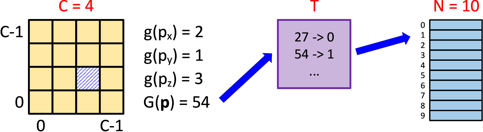 Figure 1
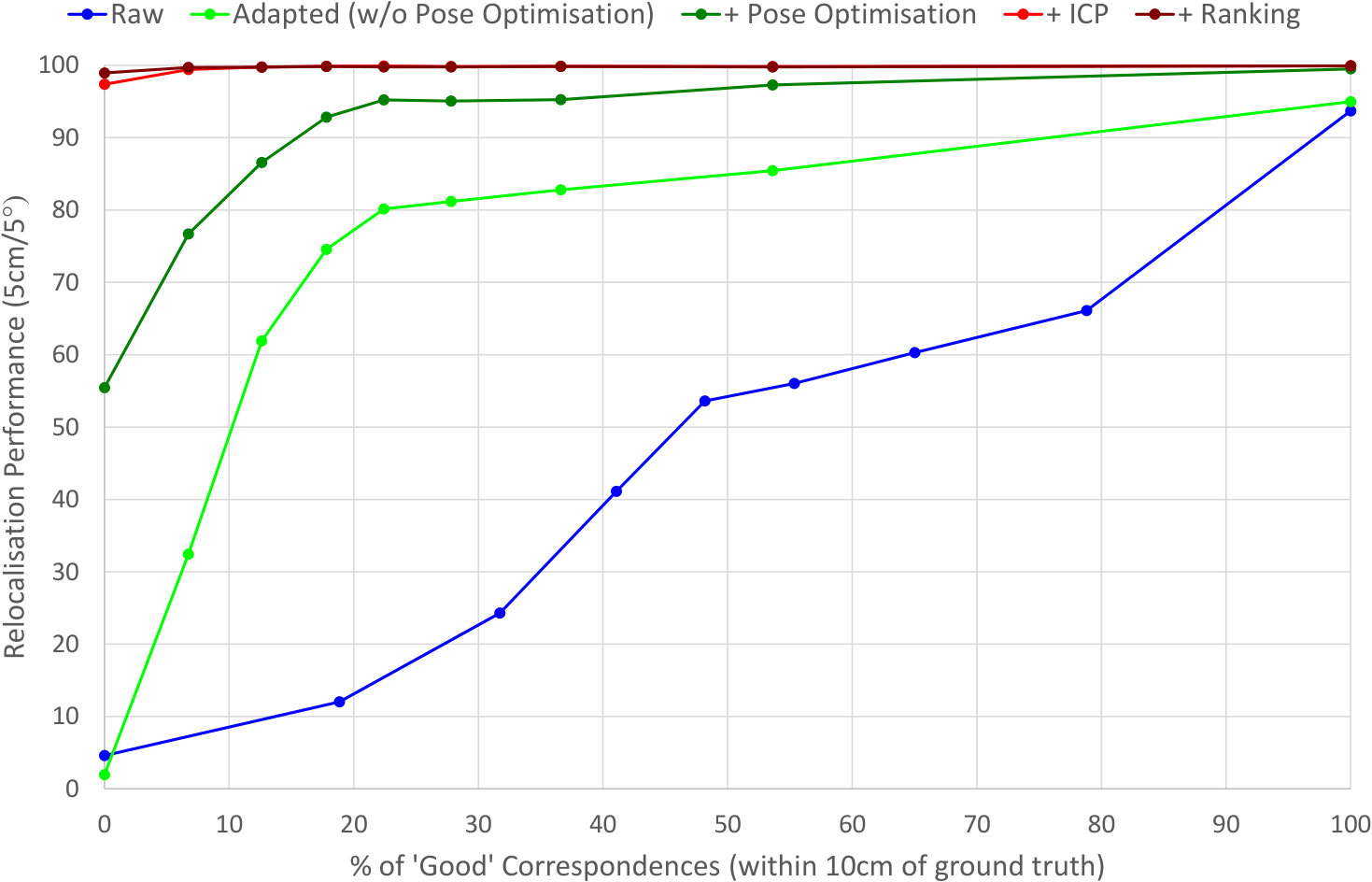 Figure 2
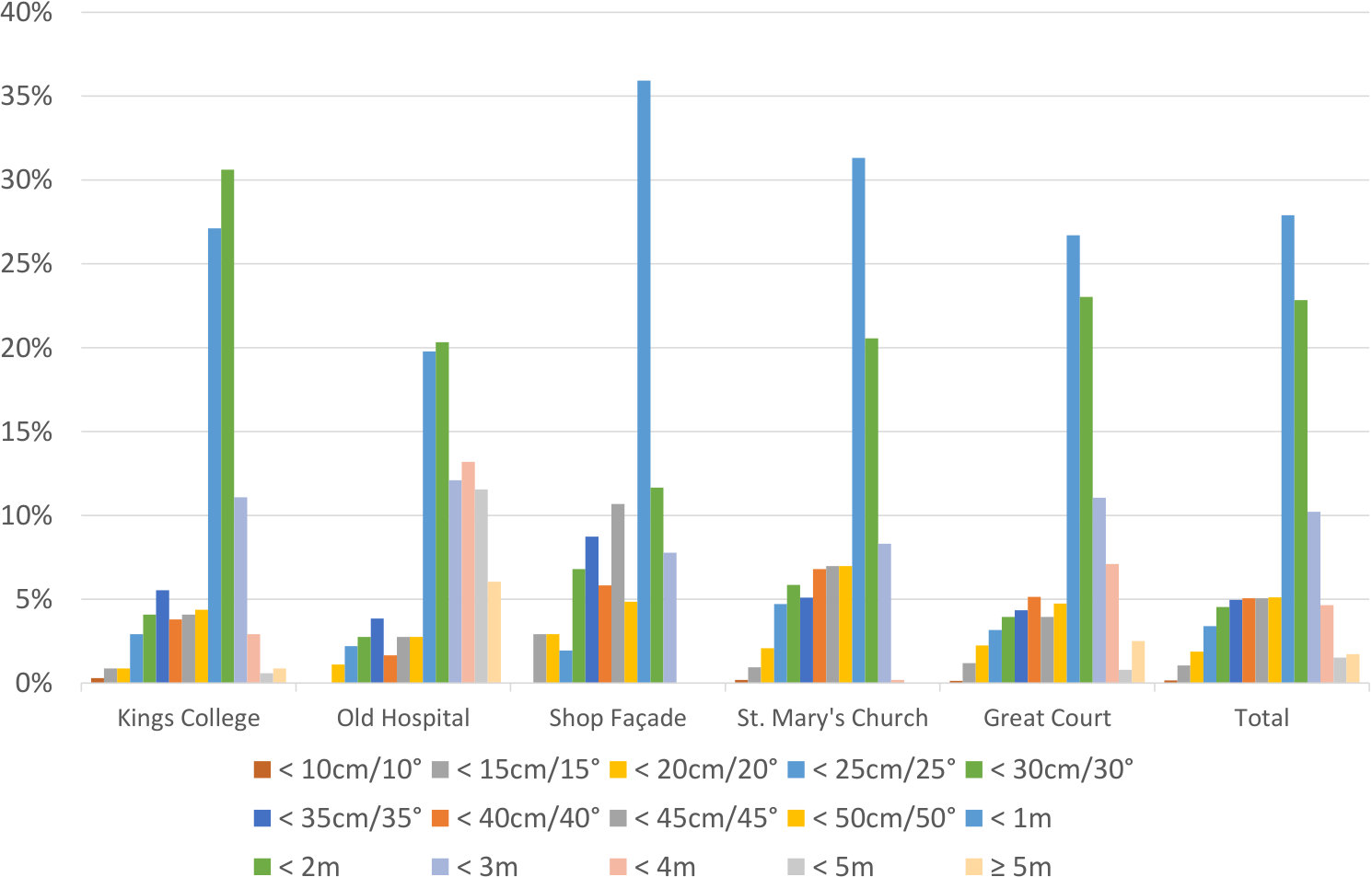 Figure 3
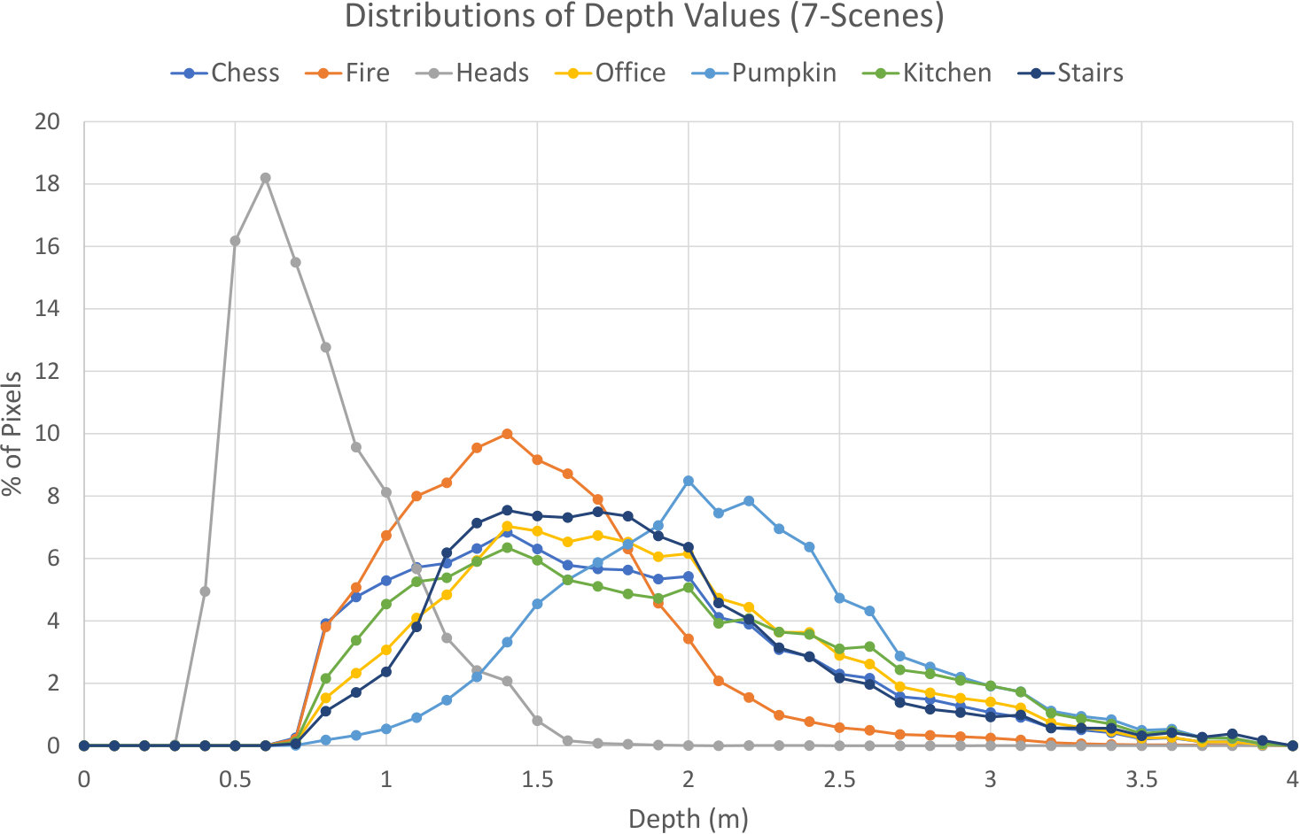 Figure 4
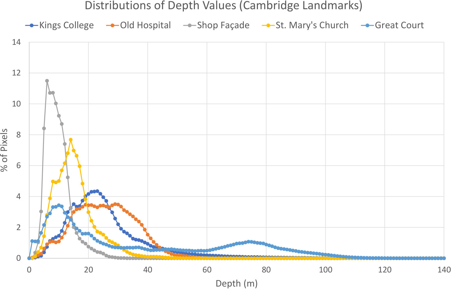 Figure 5
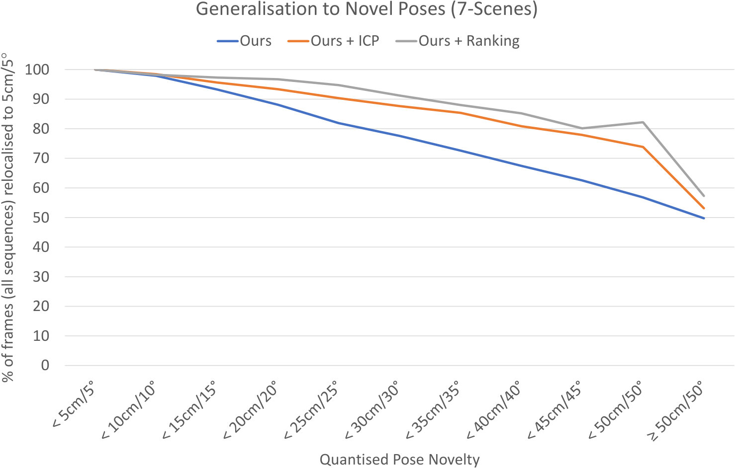 Figure 6
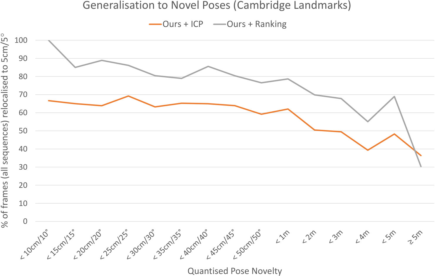 Figure 7
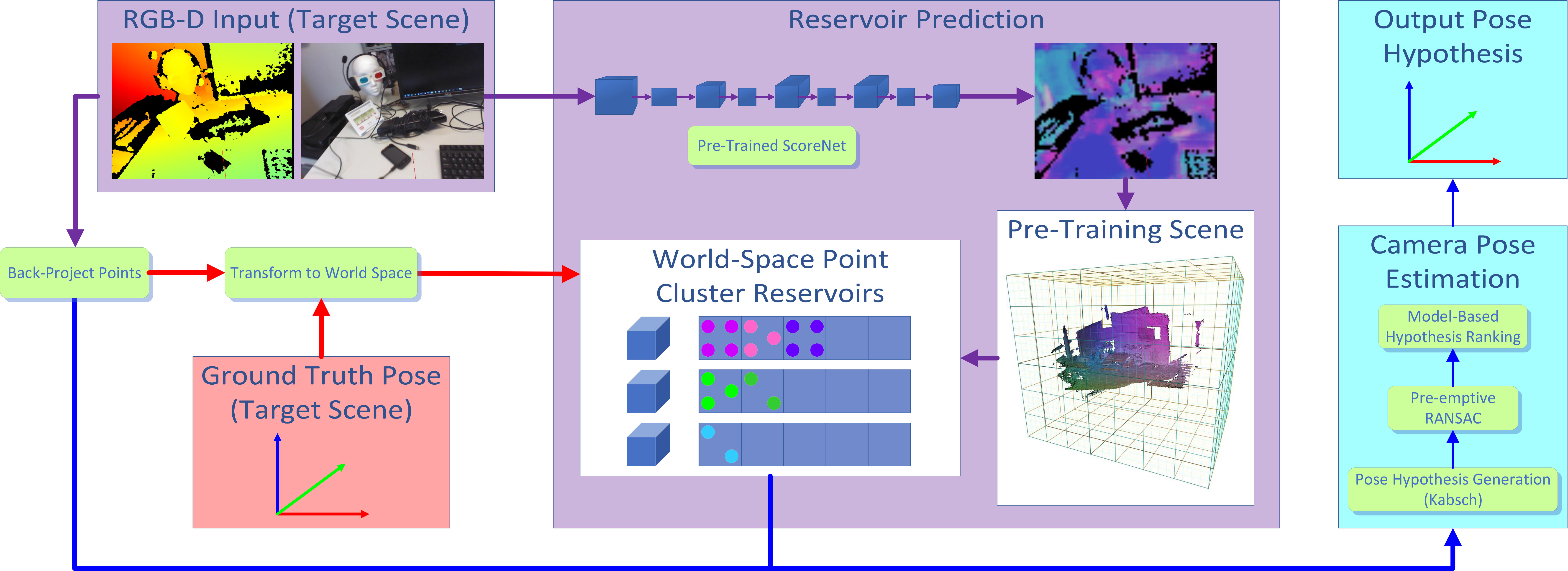 Figure 8
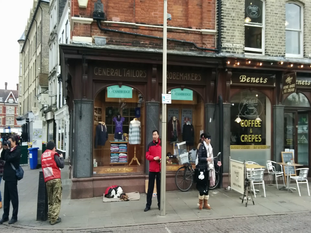 Figure 9
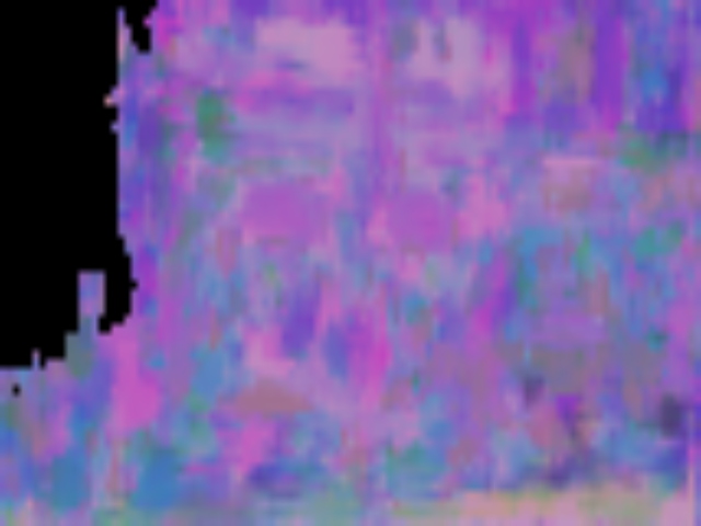 Figure 10
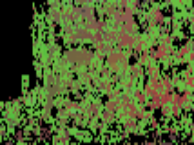 Figure 11
 Figure 12
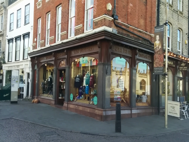 Figure 13
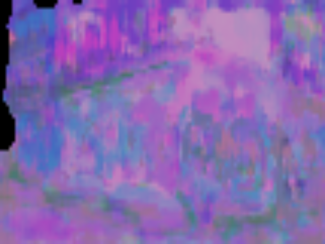 Figure 14
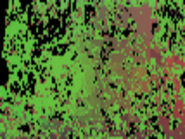 Figure 15
 Figure 16
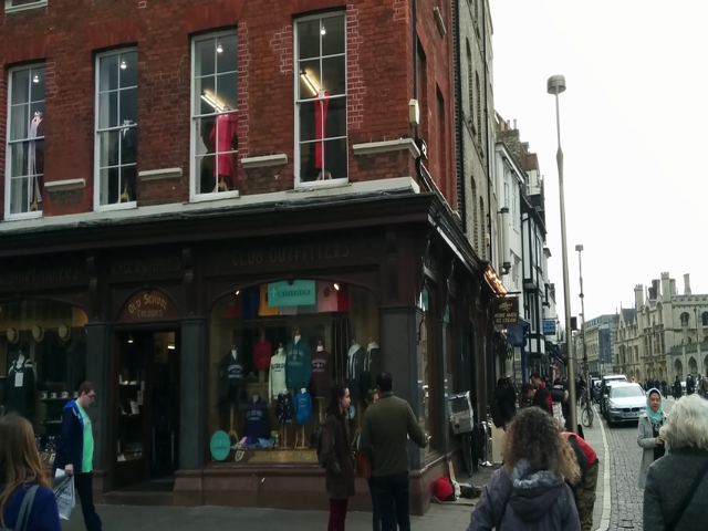 Figure 17
 Figure 18
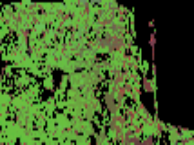 Figure 19
 Figure 20
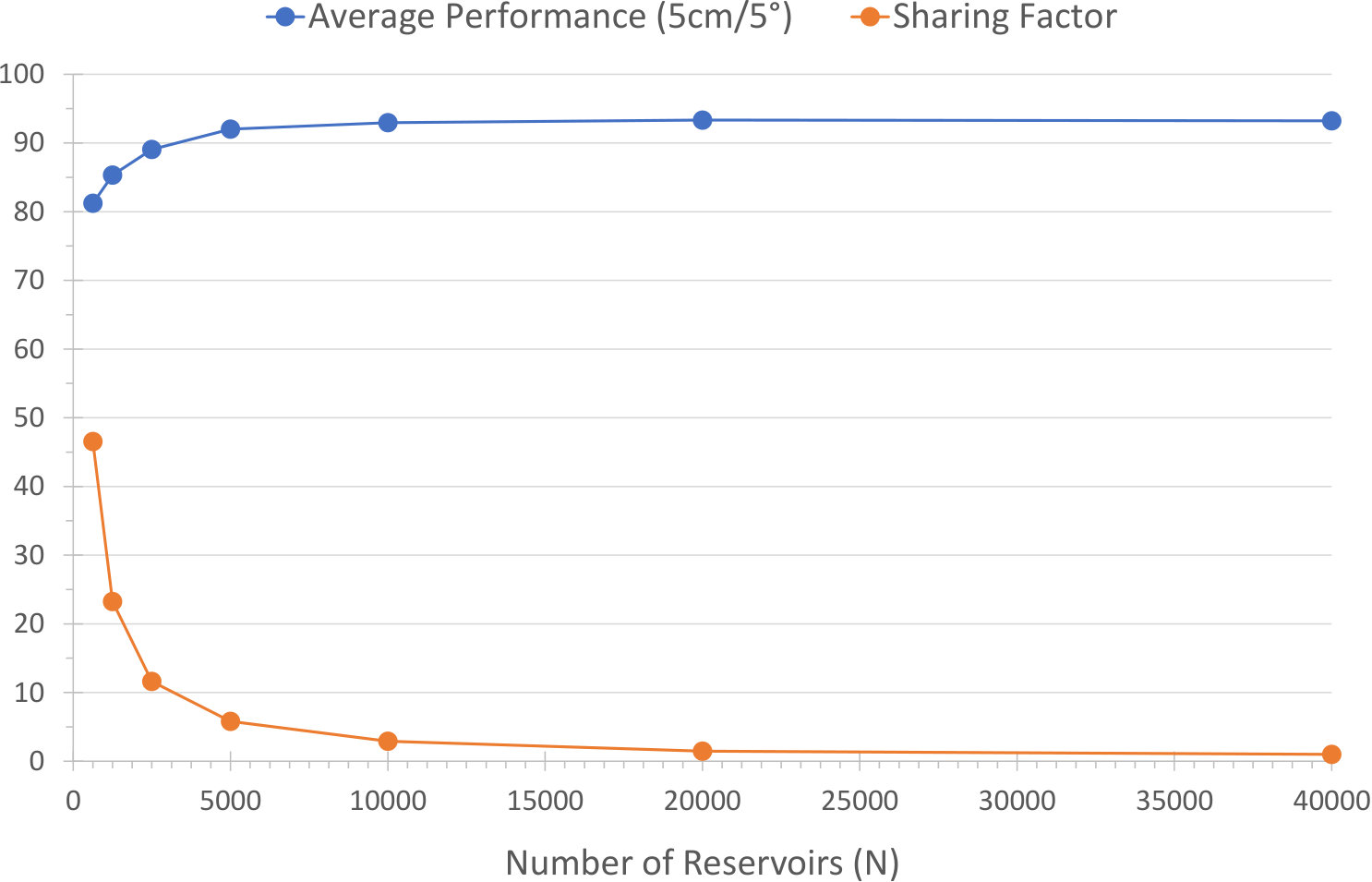 Figure 21
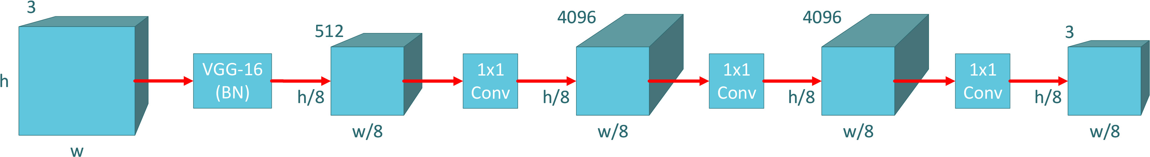 Figure 22
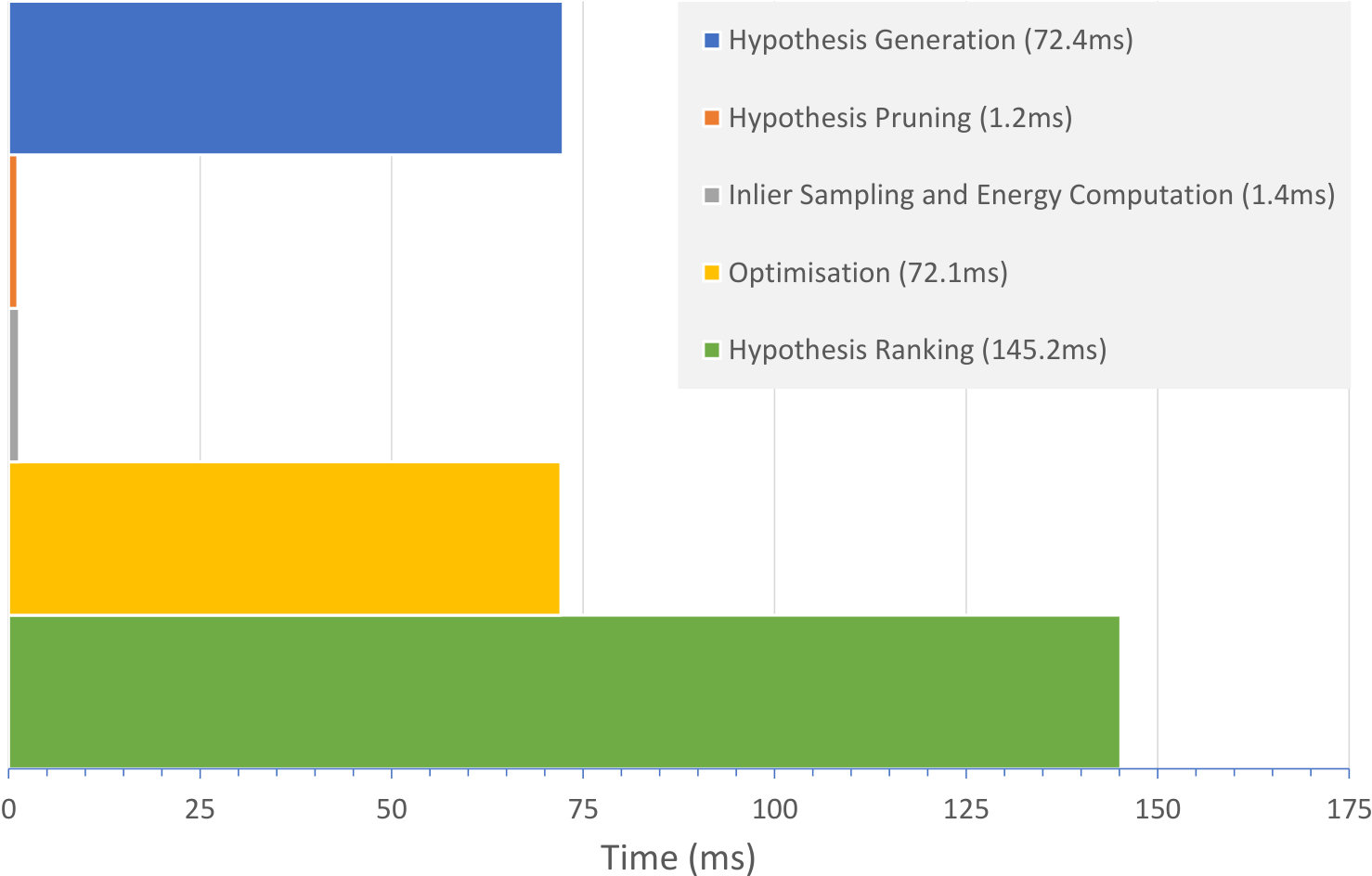 Figure 23
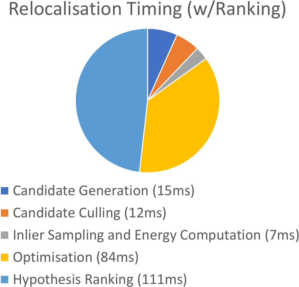 Figure 24
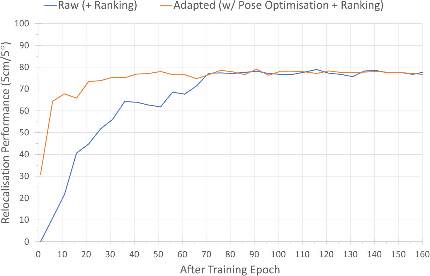 Figure 25
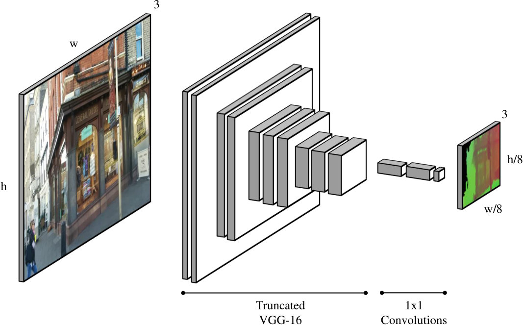 Figure 26
| Indoor Scenes | Chess | Fire | Heads | Office | Pumpkin | Kitchen | Stairs | Average | Avg. Med. Error | |
|---|---|---|---|---|---|---|---|---|---|---|
| RGB-D, online | ||||||||||
| Ours (Office) | 98.95% | 98.50% | 99.10% | 99.78% | 89.70% | 84.88% | 81.60% | 93.22% | 0.013m/1.18∘ | |
| Ours (Great Court) | 97.85% | 97.20% | 96.80% | 91.95% | 84.75% | 79.86% | 73.60% | 88.86% | 0.019m/1.06∘ | |
| Cavallari et al. [12] | 99.95% | 99.70% | 100% | 99.48% | 90.85% | 90.68% | 94.20% | 96.41% | 0.013m/1.17∘ | |
| RGB-D, offline | ||||||||||
| Ours (Offline) | 99.80% | 100% | N/A | 99.78% | 90.85% | 90.36% | 83.50% | 94.05% | 0.015m/1.08∘ | |
| Shotton et al. [63] | 92.6% | 82.9% | 49.4% | 74.9% | 73.7% | 71.8% | 27.8% | 67.6% | – | |
| Guzman-Rivera et al. [27] | 96% | 90% | 56% | 92% | 80% | 86% | 55% | 79.3% | – | |
| Valentin et al. [69] | 99.4% | 94.6% | 95.9% | 97.0% | 85.1% | 89.3% | 63.4% | 89.5% | – | |
| Brachmann et al. [6] | 99.6% | 94.0% | 89.3% | 93.4% | 77.6% | 91.1% | 71.7% | 88.1% | 0.061m/2.7∘ | |
| Meng et al. [50] | 99.5% | 97.6% | 95.5% | 96.2% | 81.4% | 89.3% | 72.2% | 90.3% | 0.017m/0.70∘ | |
| Schmidt et al. [61] | 97.75% | 96.55% | 99.8% | 97.2% | 81.4% | 93.4% | 77.7% | 92.0% | – | |
| Brachmann and Rother [7] | 97.1% | 89.6% | 92.4% | 86.6% | 59.0% | 66.6% | 29.3% | 76.1% | 0.036m/1.1∘ | |
| RGB-only, offline | ||||||||||
| Brachmann and Rother [7] | 93.8% | 75.6% | 18.4% | 75.4% | 55.9% | 50.7% | 2.0% | 60.4% | 0.084m/2.4∘ | |
| Li et al. [43] | 96.1% | 88.6% | 86.9% | 80.6% | 60.3% | 61.9% | 11.3% | 71.8% | 0.043m/1.3∘ |
| Outdoor Scenes | Kings College | Old Hospital | Shop Façade | St. Mary’s Church | Great Court |
| Online | |||||
| Ours (Great Court) | 0.011m/0.056∘ | 0.010m/0.056∘ | 0.009m/0.040∘ | 0.011m/0.056∘ | 0.018m/0.040∘ |
| 76.97% | 66.48% | 95.15% | 67.17% | 77.50% | |
| Cavallari et al. [12] | |||||
| – Office, RGB-D features | 0.01m/0.06∘ | 0.01m/0.04∘ | 0.01m/0.04∘ | 0.01m/0.06∘ | |
| (results from [12]) | 76.97% | 82.97% | 99.03% | 79.62% | |
| – Great Court, RGB-D features. | – | – | 0.009m/0.040∘ | – | – |
| (trained by us) | 35.86% | 41.21% | 94.18% | 7.55% | 0% |
| – Great Court, RGB features | – | – | 0.011m/0.056∘ | – | – |
| (trained by us) | 27.41% | 4.40% | 74.76% | 30.94% | 16.58% |
| Offline | |||||
| Ours (Offline) | 0.008m/0.040∘ | 0.008m/0.040∘ | 0.009m/0.040∘ | 0.009m/0.040∘ | 0.018m/0.040∘ |
| 99.71% | 100% | 100% | 99.62% | 77.50% | |
| PoseNet (Geom. Loss) [35] | 0.99m/1.1∘ | 2.17m/2.9∘ | 1.05m/4.0∘ | 1.49m/3.4∘ | 7.00m/3.7∘ |
| Active Search (SIFT) [59] | 0.42m/0.6∘ | 0.44m/1.0∘ | 0.12m/0.4∘ | 0.19m/0.5∘ | |
| DSAC (RGB Training) [5] | *0.30m/0.5∘ | 0.33m/0.6∘ | 0.09m/0.4∘ | *0.55m/1.6∘ | *2.80m/1.5∘ |
| DSAC++ [7] | 0.18m/0.3∘ | 0.20m/0.3∘ | 0.06m/0.3∘ | 0.13m/0.4∘ | 0.40m/0.2∘ |
| N | 625 | 1250 | 2500 | 5000 | 10000 | 20000 | 40000 |
|---|---|---|---|---|---|---|---|
| % (5cm/5∘) | 81.21 | 85.31 | 89.07 | 92.02 | 92.95 | 93.34 | 93.22 |
| Step | Time (ms) |
|---|---|
| Hypothesis Generation | 72.4 |
| Hypothesis Pruning | 1.2 |
| Inlier Sampling and Energy Computation | 1.4 |
| Optimisation | 72.1 |
| Hypothesis Ranking | 145.2 |
| Total | 292.3 |
| Name | 7-Scenes | Cambridge Landmarks |
| clustererSigma | 0.1 | 0.1 |
| clustererTau | 0.05 | 0.4 |
| maxClusterCount | 50 | 50 |
| minClusterSize | 20 | 5 |
| reservoirCapacity | 4096 | 4096 |
| maxCandidateGenerationIterations | 6000 | 6000 |
| maxPoseCandidates () | 1024 | 2048 |
| maxPoseCandidatesAfterCull () | 64 | 64 |
| maxTranslationErrorForCorrectPose | 0.05 | 0.1 |
| minSquaredDistanceBetweenSampledModes | 0.09 | 0.0225 |
| poseUpdate | True | True |
| ransacInliersPerIteration () | 512 | 512 |
| usePredictionCovarianceForPoseOptimization | True | False |
| Chess | Fire | Office | Pumpkin | Kitchen | Stairs | |
|---|---|---|---|---|---|---|
| Raw | 72.50% | 41.50% | 53.38% | 44.40% | 39.90% | 1.20% |
| 0.032m/1.495∘ | 0.061m/2.724∘ | 0.046m/1.804∘ | 0.060m/1.865∘ | 0.068m/2.255∘ | 0.528m/6.487∘ | |
| + ICP | 98.35% | 76.65% | 84.05% | 74.10% | 70.90% | 26.10% |
| 0.013m/1.034∘ | 0.009m/1.043∘ | 0.010m/1.008∘ | 0.018m/1.108∘ | 0.030m/1.480∘ | 0.552m/1.256∘ | |
| + Ranking | 98.95% | 88.85% | 90.80% | 78.35% | 79.42% | 35.40% |
| 0.013m/1.032∘ | 0.008m/1.004∘ | 0.010m/0.985∘ | 0.017m/1.096∘ | 0.027m/1.441∘ | 0.283m/1.184∘ |
| Chess | Fire | Heads | Office | Pumpkin | Kitchen | Stairs | Average | |
|---|---|---|---|---|---|---|---|---|
| Trained on: | ||||||||
| Chess | 98.65% | 90.10% | 93.00% | 84.50% | 71.45% | 84.88% | 31.50% | 79.15% |
| 0.011m/1.031∘ | 0.011m/1.049∘ | 0.010m/1.846∘ | 0.019m/1.145∘ | 0.021m/1.161∘ | 0.022m/1.439∘ | 0.260m/2.127∘ | 0.051m/1.400∘ | |
| + ICP | 99.60% | 96.90% | 97.30% | 94.88% | 89.00% | 87.24% | 49.20% | 87.73% |
| 0.013m/1.033∘ | 0.007m/0.968∘ | 0.003m/1.698∘ | 0.009m/0.957∘ | 0.016m/1.070∘ | 0.025m/1.418∘ | 0.234m/1.099∘ | 0.044m/1.178∘ | |
| + Ranking | 99.80% | 97.60% | 99.00% | 97.80% | 90.15% | 86.40% | 78.00% | 92.68% |
| 0.013m/1.031∘ | 0.008m/0.991∘ | 0.003m/1.701∘ | 0.010m/0.960∘ | 0.016m/1.073∘ | 0.025m/1.436∘ | 0.020m/1.056∘ | 0.014m/1.179∘ | |
| Fire | 96.80% | 89.85% | 95.70% | 88.55% | 73.40% | 83.68% | 33.20% | 80.17% |
| 0.010m/1.039∘ | 0.012m/1.058∘ | 0.008m/1.823∘ | 0.017m/1.109∘ | 0.020m/1.143∘ | 0.022m/1.444∘ | 0.260m/1.686∘ | 0.050m/1.329∘ | |
| + ICP | 98.55% | 99.90% | 98.30% | 96.60% | 85.55% | 87.50% | 51.10% | 88.21% |
| 0.013m/1.032∘ | 0.007m/0.962∘ | 0.003m/1.698∘ | 0.009m/0.950∘ | 0.016m/1.070∘ | 0.025m/1.419∘ | 0.030m/1.064∘ | 0.015m/1.171∘ | |
| + Ranking | 98.70% | 100.00% | 99.40% | 98.05% | 89.35% | 85.92% | 82.30% | 93.39% |
| 0.014m/1.048∘ | 0.008m/0.970∘ | 0.003m/1.701∘ | 0.009m/0.955∘ | 0.017m/1.073∘ | 0.025m/1.434∘ | 0.019m/1.051∘ | 0.013m/1.176∘ | |
| Office | 96.65% | 88.05% | 90.80% | 95.17% | 67.00% | 80.02% | 25.90% | 77.66% |
| 0.010m/1.048∘ | 0.013m/1.061∘ | 0.012m/1.948∘ | 0.013m/1.032∘ | 0.024m/1.194∘ | 0.024m/1.470∘ | 0.311m/2.002∘ | 0.058m/1.393∘ | |
| + ICP | 98.80% | 97.85% | 97.50% | 99.88% | 84.60% | 85.12% | 39.10% | 86.12% |
| 0.013m/1.036∘ | 0.007m/0.969∘ | 0.003m/1.702∘ | 0.009m/0.941∘ | 0.017m/1.074∘ | 0.026m/1.417∘ | 0.280m/1.164∘ | 0.051m/1.186∘ | |
| + Ranking | 98.95% | 98.50% | 99.10% | 99.78% | 89.70% | 84.88% | 81.60% | 93.22% |
| 0.013m/1.036∘ | 0.008m/0.985∘ | 0.003m/1.704∘ | 0.009m/0.943∘ | 0.016m/1.071∘ | 0.025m/1.435∘ | 0.019m/1.059∘ | 0.013m/1.176∘ | |
| Pumpkin | 96.95% | 90.90% | 84.80% | 86.70% | 72.65% | 84.92% | 26.60% | 77.65% |
| 0.011m/1.072∘ | 0.011m/1.058∘ | 0.012m/1.872∘ | 0.019m/1.136∘ | 0.020m/1.147∘ | 0.021m/1.435∘ | 0.281m/2.208∘ | 0.054m/1.418∘ | |
| + ICP | 98.05% | 98.25% | 91.70% | 97.22% | 90.30% | 87.62% | 44.20% | 86.76% |
| 0.013m/1.035∘ | 0.007m/0.965∘ | 0.003m/1.699∘ | 0.009m/0.950∘ | 0.016m/1.066∘ | 0.025m/1.418∘ | 0.272m/1.149∘ | 0.049m/1.183∘ | |
| + Ranking | 98.60% | 99.45% | 95.80% | 97.68% | 90.85% | 87.76% | 70.90% | 91.58% |
| 0.013m/1.038∘ | 0.008m/0.977∘ | 0.003m/1.704∘ | 0.009m/0.956∘ | 0.016m/1.069∘ | 0.025m/1.433∘ | 0.021m/1.068∘ | 0.014m/1.178∘ | |
| Kitchen | 96.05% | 85.80% | 89.00% | 81.10% | 69.75% | 87.20% | 17.80% | 75.24% |
| 0.012m/1.063∘ | 0.014m/1.067∘ | 0.011m/1.904∘ | 0.022m/1.166∘ | 0.025m/1.177∘ | 0.023m/1.427∘ | 0.322m/2.577∘ | 0.061m/1.483∘ | |
| + ICP | 98.35% | 95.75% | 92.30% | 92.47% | 85.85% | 90.44% | 34.70% | 84.27% |
| 0.013m/1.034∘ | 0.007m/0.967∘ | 0.003m/1.699∘ | 0.009m/0.968∘ | 0.017m/1.070∘ | 0.024m/1.410∘ | 0.281m/1.188∘ | 0.051m/1.191∘ | |
| + Ranking | 98.80% | 97.75% | 96.50% | 95.62% | 89.40% | 90.36% | 77.30% | 92.25% |
| 0.013m/1.037∘ | 0.008m/0.979∘ | 0.003m/1.703∘ | 0.009m/0.961∘ | 0.016m/1.072∘ | 0.024m/1.413∘ | 0.020m/1.058∘ | 0.013m/1.175∘ | |
| Stairs | 96.70% | 87.20% | 87.80% | 86.75% | 70.20% | 79.72% | 46.20% | 79.22% |
| 0.011m/1.059∘ | 0.013m/1.059∘ | 0.011m/1.874∘ | 0.018m/1.116∘ | 0.022m/1.193∘ | 0.027m/1.501∘ | 0.073m/1.304∘ | 0.025m/1.301∘ | |
| + ICP | 98.45% | 96.85% | 95.80% | 96.38% | 81.65% | 85.74% | 56.20% | 87.30% |
| 0.013m/1.033∘ | 0.007m/0.971∘ | 0.003m/1.701∘ | 0.009m/0.952∘ | 0.017m/1.076∘ | 0.025m/1.420∘ | 0.023m/1.053∘ | 0.014m/1.172∘ | |
| + Ranking | 98.70% | 97.80% | 97.80% | 97.88% | 86.25% | 84.86% | 83.50% | 92.40% |
| 0.013m/1.043∘ | 0.008m/0.993∘ | 0.003m/1.704∘ | 0.010m/0.957∘ | 0.016m/1.072∘ | 0.025m/1.438∘ | 0.018m/1.037∘ | 0.013m/1.178∘ |
| Kings College | Old Hospital | Shop Façade | St. Mary’s Church | Great Court | |
|---|---|---|---|---|---|
| Raw | 2.04% | 1.10% | 0.00% | 0.19% | 0.13% |
| 0.308m/0.588∘ | 0.514m/0.693∘ | 0.769m/3.265∘ | 0.504m/1.797∘ | 0.785m/0.884∘ | |
| + ICP | 95.04% | 100% | 89.32% | 94.15% | 52.37% |
| 0.009m/0.040∘ | 0.008m/0.000∘ | 0.008m/0.040∘ | 0.009m/0.040∘ | 0.028m/0.079∘ | |
| + Ranking | 99.13% | 100% | 96.12% | 99.62% | 79.34% |
| 0.008m/0.040∘ | 0.008m/0.040∘ | 0.008m/0.056∘ | 0.009m/0.040∘ | 0.017m/0.040∘ |
| Kings College | Old Hospital | Shop Façade | St. Mary’s Church | Great Court | Average | |
|---|---|---|---|---|---|---|
| Trained on: | ||||||
| Kings College | 6.41% | 0.55% | 2.91% | 0.75% | 0.13% | 2.15% |
| 0.137m/0.444∘ | 0.955m/2.565∘ | 0.273m/1.721∘ | 5.345m/17.904∘ | 33.042m/85.858∘ | ||
| + ICP | 97.08% | 80.22% | 96.12% | 48.11% | 25.26% | 69.36% |
| 0.018m/0.069∘ | 0.010m/0.056∘ | 0.014m/0.056∘ | 5.345m/11.121∘ | 33.042m/85.858∘ | ||
| + Ranking | 99.71% | 85.16% | 100.00% | 76.98% | 31.18% | 78.61% |
| 0.008m/0.040∘ | 0.009m/0.040∘ | 0.008m/0.040∘ | 0.011m/0.056∘ | 31.972m/81.311∘ | ||
| Old Hospital | 0.29% | 5.49% | 1.94% | 0.00% | 0.13% | 1.57% |
| 1.146m/4.279∘ | 0.169m/0.407∘ | 0.308m/2.061∘ | 2.228m/11.877∘ | 37.432m/113.246∘ | ||
| + ICP | 65.31% | 99.45% | 95.15% | 53.21% | 8.42% | 64.31% |
| 0.013m/0.056∘ | 0.008m/0.040∘ | 0.008m/0.056∘ | 0.021m/0.088∘ | 37.432m/113.246∘ | ||
| + Ranking | 74.05% | 100.00% | 99.03% | 75.66% | 13.82% | 72.51% |
| 0.011m/0.056∘ | 0.008m/0.040∘ | 0.008m/0.040∘ | 0.010m/0.056∘ | 36.278m/108.150∘ | ||
| Shop Façade | 0.00% | 0.00% | 6.80% | 0.00% | 0.00% | 1.36% |
| 4.557m/11.934∘ | 1.533m/3.879∘ | 0.157m/0.989∘ | 2.107m/13.161∘ | 35.936m/108.056∘ | ||
| + ICP | 46.06% | 62.64% | 100.00% | 56.23% | 12.24% | 55.43% |
| 3.482m/7.200∘ | 0.010m/0.069∘ | 0.008m/0.040∘ | 0.015m/0.079∘ | 35.936m/108.056∘ | ||
| + Ranking | 75.22% | 76.37% | 100.00% | 70.94% | 14.87% | 67.48% |
| 0.011m/0.056∘ | 0.009m/0.056∘ | 0.009m/0.040∘ | 0.011m/0.056∘ | 33.772m/102.254∘ | ||
| St. Mary’s Church | 0.87% | 0.55% | 1.94% | 5.66% | 0.00% | 1.80% |
| 0.679m/2.601∘ | 0.898m/2.527∘ | 0.242m/1.666∘ | 0.181m/0.845∘ | 39.341m/119.539∘ | ||
| + ICP | 74.05% | 79.67% | 97.09% | 94.91% | 9.21% | 70.99% |
| 0.012m/0.056∘ | 0.009m/0.040∘ | 0.009m/0.040∘ | 0.009m/0.040∘ | 39.341m/119.539∘ | ||
| + Ranking | 81.63% | 82.97% | 99.03% | 99.62% | 17.37% | 76.12% |
| 0.011m/0.056∘ | 0.009m/0.040∘ | 0.008m/0.040∘ | 0.009m/0.040∘ | 37.587m/110.541∘ | ||
| Great Court | 0.29% | 0.00% | 0.97% | 0.75% | 0.79% | 0.56% |
| 0.954m/3.390∘ | 2.225m/5.216∘ | 0.481m/3.112∘ | 11.726m/46.959∘ | 0.710m/1.671∘ | ||
| + ICP | 72.89% | 59.34% | 77.67% | 39.25% | 58.95% | 61.62% |
| 0.011m/0.056∘ | 0.011m/0.056∘ | 0.009m/0.056∘ | 11.726m/46.959∘ | 0.022m/0.069∘ | ||
| + Ranking | 76.97% | 66.48% | 95.15% | 67.17% | 77.50% | 76.65% |
| 0.011m/0.056∘ | 0.010m/0.056∘ | 0.009m/0.040∘ | 0.011m/0.056∘ | 0.018m/0.040∘ |
| Chess | Fire | Heads | Office | Pumpkin | Kitchen | Stairs | Average | |
|---|---|---|---|---|---|---|---|---|
| Trained on: | ||||||||
| Kings College | 93.70% | 81.85% | 86.50% | 76.17% | 60.95% | 69.76% | 17.00% | 69.42% |
| 0.012m/1.097∘ | 0.017m/1.134∘ | 0.011m/1.917∘ | 0.026m/1.259∘ | 0.031m/1.326∘ | 0.033m/1.588∘ | 0.352m/3.798∘ | 0.069m/1.731∘ | |
| + ICP | 97.05% | 93.15% | 90.60% | 88.07% | 76.55% | 81.58% | 43.00% | 81.43% |
| 0.013m/1.037∘ | 0.007m/0.971∘ | 0.003m/1.700∘ | 0.010m/0.986∘ | 0.017m/1.087∘ | 0.026m/1.423∘ | 0.283m/1.261∘ | 0.051m/1.209∘ | |
| + Ranking | 98.10% | 96.15% | 93.50% | 91.55% | 81.90% | 81.20% | 59.10% | 85.93% |
| 0.013m/1.046∘ | 0.008m/0.988∘ | 0.003m/1.702∘ | 0.010m/0.986∘ | 0.017m/1.084∘ | 0.026m/1.441∘ | 0.024m/1.108∘ | 0.015m/1.194∘ | |
| Old Hospital | 94.70% | 86.70% | 90.10% | 77.68% | 67.15% | 76.10% | 26.10% | 74.08% |
| 0.012m/1.092∘ | 0.013m/1.067∘ | 0.009m/1.814∘ | 0.023m/1.218∘ | 0.024m/1.234∘ | 0.027m/1.530∘ | 0.281m/2.513∘ | 0.056m/1.495∘ | |
| + ICP | 97.70% | 94.35% | 93.10% | 90.38% | 77.20% | 83.72% | 48.50% | 83.56% |
| 0.013m/1.034∘ | 0.007m/0.974∘ | 0.003m/1.700∘ | 0.009m/0.972∘ | 0.017m/1.078∘ | 0.026m/1.422∘ | 0.263m/1.093∘ | 0.048m/1.182∘ | |
| + Ranking | 98.05% | 96.90% | 93.60% | 93.00% | 82.30% | 82.84% | 75.80% | 88.93% |
| 0.013m/1.039∘ | 0.008m/0.991∘ | 0.003m/1.703∘ | 0.010m/0.976∘ | 0.017m/1.081∘ | 0.026m/1.439∘ | 0.020m/1.056∘ | 0.014m/1.184∘ | |
| Shop Façade | 93.20% | 86.90% | 92.50% | 77.07% | 67.85% | 76.48% | 24.70% | 74.10% |
| 0.011m/1.080∘ | 0.012m/1.069∘ | 0.010m/1.845∘ | 0.022m/1.196∘ | 0.025m/1.211∘ | 0.026m/1.513∘ | 0.289m/2.405∘ | 0.056m/1.474∘ | |
| + ICP | 97.50% | 96.25% | 98.40% | 91.47% | 81.10% | 84.64% | 44.50% | 84.84% |
| 0.013m/1.036∘ | 0.007m/0.970∘ | 0.003m/1.700∘ | 0.009m/0.970∘ | 0.017m/1.073∘ | 0.026m/1.420∘ | 0.272m/1.109∘ | 0.050m/1.182∘ | |
| + Ranking | 98.20% | 98.20% | 99.30% | 95.15% | 85.10% | 83.48% | 73.70% | 90.45% |
| 0.014m/1.052∘ | 0.008m/0.999∘ | 0.003m/1.705∘ | 0.010m/0.968∘ | 0.017m/1.077∘ | 0.026m/1.443∘ | 0.021m/1.067∘ | 0.014m/1.187∘ | |
| St. Mary’s Church | 94.00% | 76.70% | 82.10% | 78.15% | 55.90% | 70.60% | 9.30% | 66.68% |
| 0.013m/1.104∘ | 0.021m/1.143∘ | 0.013m/2.024∘ | 0.024m/1.232∘ | 0.041m/1.429∘ | 0.031m/1.563∘ | 0.575m/5.759∘ | 0.103m/2.036∘ | |
| + ICP | 97.35% | 93.15% | 87.90% | 92.43% | 71.85% | 80.38% | 24.20% | 78.18% |
| 0.013m/1.036∘ | 0.007m/0.975∘ | 0.003m/1.705∘ | 0.009m/0.963∘ | 0.018m/1.105∘ | 0.027m/1.426∘ | 0.564m/1.416∘ | 0.092m/1.232∘ | |
| + Ranking | 98.30% | 96.45% | 93.90% | 95.65% | 80.40% | 81.78% | 50.20% | 85.24% |
| 0.013m/1.039∘ | 0.008m/0.993∘ | 0.003m/1.702∘ | 0.010m/0.960∘ | 0.017m/1.085∘ | 0.026m/1.438∘ | 0.037m/1.140∘ | 0.016m/1.194∘ | |
| Great Court | 92.50% | 85.25% | 88.90% | 73.70% | 63.10% | 66.20% | 24.40% | 70.58% |
| 0.012m/1.096∘ | 0.013m/1.082∘ | 0.011m/1.883∘ | 0.026m/1.290∘ | 0.032m/1.318∘ | 0.035m/1.637∘ | 0.314m/2.524∘ | 0.063m/1.547∘ | |
| + ICP | 96.80% | 95.10% | 94.50% | 87.75% | 77.25% | 79.42% | 41.30% | 81.73% |
| 0.013m/1.038∘ | 0.007m/0.973∘ | 0.003m/1.701∘ | 0.010m/0.984∘ | 0.017m/1.085∘ | 0.027m/1.425∘ | 0.281m/1.185∘ | 0.051m/1.199∘ | |
| + Ranking | 97.85% | 97.20% | 96.80% | 91.95% | 84.75% | 79.86% | 73.60% | 88.86% |
| 0.015m/1.060∘ | 0.008m/0.996∘ | 0.003m/1.704∘ | 0.010m/0.985∘ | 0.018m/1.104∘ | 0.026m/1.446∘ | 0.019m/1.056∘ | 0.014m/1.193∘ |
| Kings College | Old Hospital | Shop Façade | St. Mary’s Church | Great Court | Average | |
|---|---|---|---|---|---|---|
| Trained on: | ||||||
| Chess | 0.00% | 0.55% | 5.83% | 0.00% | 0.00% | 1.28% |
| 2.431m/6.882∘ | 1.463m/3.256∘ | 0.240m/1.735∘ | 7.068m/31.042∘ | 38.155m/113.588∘ | ||
| + ICP | 51.02% | 68.13% | 100.00% | 43.21% | 8.68% | 54.21% |
| 0.026m/0.097∘ | 0.009m/0.056∘ | 0.008m/0.040∘ | 7.068m/30.908∘ | 38.155m/113.588∘ | ||
| + Ranking | 68.51% | 77.47% | 100.00% | 71.51% | 13.16% | 66.13% |
| 0.013m/0.069∘ | 0.009m/0.056∘ | 0.008m/0.040∘ | 0.011m/0.056∘ | 34.747m/105.913∘ | ||
| Fire | 0.58% | 0.00% | 2.91% | 0.19% | 0.00% | 0.74% |
| 1.794m/6.451∘ | 1.340m/2.977∘ | 0.282m/1.921∘ | 2.131m/12.996∘ | 38.667m/114.043∘ | ||
| + ICP | 55.69% | 66.48% | 98.06% | 53.21% | 7.24% | 56.14% |
| 0.017m/0.079∘ | 0.010m/0.056∘ | 0.008m/0.040∘ | 0.019m/0.088∘ | 38.667m/114.043∘ | ||
| + Ranking | 77.26% | 84.62% | 100.00% | 73.77% | 19.61% | 71.05% |
| 0.011m/0.056∘ | 0.009m/0.040∘ | 0.008m/0.040∘ | 0.011m/0.056∘ | 35.497m/96.146∘ | ||
| Office | 0.29% | 0.55% | 5.83% | 0.19% | 0.00% | 1.37% |
| 5.997m/12.155∘ | 1.133m/2.906∘ | 0.222m/1.625∘ | 1.435m/9.180∘ | 36.601m/120.281∘ | ||
| + ICP | 48.98% | 67.58% | 94.17% | 55.47% | 7.11% | 54.66% |
| 4.215m/11.460∘ | 0.010m/0.056∘ | 0.009m/0.040∘ | 0.016m/0.069∘ | 36.601m/120.281∘ | ||
| + Ranking | 65.01% | 85.71% | 98.06% | 78.68% | 10.79% | 67.65% |
| 0.013m/0.056∘ | 0.009m/0.040∘ | 0.009m/0.040∘ | 0.010m/0.056∘ | 37.484m/119.759∘ | ||
| Pumpkin | 0.87% | 0.55% | 2.91% | 0.38% | 0.00% | 0.94% |
| 2.490m/6.705∘ | 1.576m/3.652∘ | 0.261m/1.977∘ | 27.319m/99.484∘ | 42.037m/124.438∘ | ||
| + ICP | 52.77% | 65.93% | 96.12% | 26.42% | 3.42% | 48.93% |
| 0.020m/0.079∘ | 0.010m/0.056∘ | 0.008m/0.040∘ | 27.319m/99.484∘ | 42.037m/124.438∘ | ||
| + Ranking | 61.22% | 74.73% | 98.06% | 75.85% | 8.42% | 63.66% |
| 0.013m/0.069∘ | 0.009m/0.056∘ | 0.008m/0.040∘ | 0.010m/0.056∘ | 41.110m/122.393∘ | ||
| Kitchen | 0.00% | 0.00% | 2.91% | 0.38% | 0.00% | 0.66% |
| 20.956m/40.494∘ | 1.177m/2.984∘ | 0.223m/1.589∘ | 20.186m/79.515∘ | 41.690m/120.167∘ | ||
| + ICP | 44.02% | 64.84% | 95.15% | 38.30% | 7.11% | 49.88% |
| 20.956m/40.494∘ | 0.010m/0.056∘ | 0.009m/0.040∘ | 20.186m/79.515∘ | 41.690m/120.167∘ | ||
| + Ranking | 54.81% | 76.37% | 99.03% | 62.83% | 9.87% | 60.58% |
| 0.018m/0.079∘ | 0.009m/0.056∘ | 0.008m/0.040∘ | 0.013m/0.069∘ | 40.064m/125.348∘ | ||
| Stairs | 0.29% | 0.55% | 5.83% | 0.38% | 0.00% | 1.41% |
| 7.680m/20.316∘ | 1.113m/2.779∘ | 0.250m/2.017∘ | 1.503m/8.894∘ | 38.856m/116.153∘ | ||
| + ICP | 45.48% | 68.68% | 89.32% | 54.34% | 5.39% | 52.64% |
| 7.019m/20.238∘ | 0.009m/0.056∘ | 0.009m/0.056∘ | 0.016m/0.079∘ | 38.856m/116.153∘ | ||
| + Ranking | 67.35% | 78.02% | 99.03% | 70.75% | 12.50% | 65.53% |
| 0.012m/0.056∘ | 0.009m/0.040∘ | 0.009m/0.040∘ | 0.011m/0.056∘ | 37.474m/112.747∘ |
Peer Reviews
No public reviews on file for this paper yet. If you reviewed it on a platform where reviews are public (OpenReview, ICLR, NeurIPS, ICML), you can paste yours below so the community can read it here.
Videos
No videos yet. Explain this paper in a talk, walkthrough, or lecture? Add one.
Let’s Take This Online: Adapting Scene Coordinate Regression
Network Predictions for Online RGB-D Camera Relocalisation
Tommaso Cavallari1, Luca Bertinetto1 Jishnu Mukhoti1
Philip Torr1,2 Stuart Golodetz1,∗
1 Oxford Research Group, FiveAI Ltd.
2 Department of Engineering Science, University of Oxford
{tommaso.cavallari,luca.bertinetto,jishnu.mukhoti,stuart}@five.ai
[email protected] Authors contributed equally.
Abstract
Many applications require a camera to be relocalised online, without expensive offline training on the target scene. Whilst both keyframe and sparse keypoint matching methods can be used online, the former often fail away from the training trajectory, and the latter can struggle in textureless regions. By contrast, scene coordinate regression (SCoRe) methods generalise to novel poses and can leverage dense correspondences to improve robustness, and recent work has shown how to adapt SCoRe forests between scenes, allowing their state-of-the-art performance to be leveraged online. However, because they use features hand-crafted for indoor use, they do not generalise well to harder outdoor scenes. Whilst replacing the forest with a neural network and learning suitable features for outdoor use is possible, the techniques used to adapt forests between scenes are unfortunately harder to transfer to a network context. In this paper, we address this by proposing a novel way of leveraging a network trained on one scene to predict points in another scene. Our approach replaces the appearance clustering performed by the branching structure of a regression forest with a two-step process that first uses the network to predict points in the original scene, and then uses these predicted points to look up clusters of points from the new scene. We show experimentally that our online approach achieves state-of-the-art performance on both the 7-Scenes and Cambridge Landmarks datasets, whilst running in under 300ms, making it highly effective in live scenarios.
1 Introduction
Visual-only camera relocalisation has a wide variety of applications across computer vision and robotics, including augmented reality [11, 55, 26, 58, 2], tracking recovery and loop closure during SLAM [71, 52, 12], and map merging [33, 25]. For many applications, an ability to relocalise a camera online, i.e. without expensive prior training on the scene of interest, is critical. For example, in an interactive SLAM context, it is typical to initialise the pose of the camera at the start of reconstruction and then track it from one frame to the next, but when that tracking inevitably fails at some point, it is important to be able to relocalise the camera as soon as possible so that reconstruction can continue without unnecessary delay. However, despite the significant research attention that has been devoted to camera relocalisation in recent years, many state-of-the-art methods (especially those based on regression) remain wedded to an offline setting, making them difficult to deploy for live use. Existing methods can be broadly divided into five types:
(i) Global matching methods match one or more frames (or a descriptor, point cloud or 3D model derived from them) against either the contents of a database (e.g. one containing a map from keyframes to known poses), or a model of the scene, to look up a suitable pose. Methods like [23] match the image itself against synthetic views of the scene, whereas [22] and [24] match image descriptors against a database. Other methods [38, 3] find the nearest neighbours to a query image in the database, and use their poses to determine the query pose. Such image retrieval methods can struggle to generalise to novel poses. Geometry-based matching methods avoid this, but often require more than a single frame from which to relocalise. For example, [17] matches a point cloud constructed from a set of query images to a point cloud of the scene, whilst [44] reconstructs a 3D model from a short video sequence and matches that against the scene. One exception is [62], which matches hallucinated subvolumes against a database using a variational encoder-decoder network. This is single-frame, but quite slow, taking around a second per frame to relocalise.
(ii) Global regression methods directly regress an image’s pose, using e.g. decision forests [32], pose regression networks [36, 34, 35, 47, 72, 1], GANs [10] or LSTMs [15, 70]. Various recent approaches [9, 57, 67, 40] have made use of the relative poses between images to improve performance. Global regression methods have proved popular, but have typically struggled to achieve the accuracy of local methods (see below). Those methods that do achieve better performance [57, 67] currently do so by relying on an estimated pose from the previous frame, thereby essentially performing camera tracking rather than single-image relocalisation. Indeed, recent work by Sattler et al. [60] has shown that global regression is in many ways conceptually similar to image retrieval, and that current such approaches do not consistently outperform an image retrieval baseline or generalise well to novel poses. (This link with image retrieval was also noted earlier by Wu et al. [72].)
(iii) Local matching methods match points in camera space with known points in world space, pass the correspondences to the Perspective-n-Point (PnP) algorithm [28] or the Kabsch algorithm [31] to generate a number of initial camera pose hypotheses, and then refine these down to a final pose using some variant of RANSAC [20]. Many approaches match the descriptors of sparse keypoints to perform this matching [71, 41, 19, 59]; some approaches that perform dense matching also exist [61]. Local matching methods tend to generalise better to novel poses than image retrieval methods, since individual points are often easier to match from novel angles than are whole images.
(iv) Local regression methods generally use regression forests [63, 27, 69, 6, 48, 13, 49, 50, 12], neural networks [5, 7, 18, 42, 43, 8], or a mix of the two [46] to predict the scene coordinates of pixels in the input image. They then pass these correspondences to PnP/Kabsch and RANSAC. Compared to local matching methods, local regression methods can avoid the need for explicit keypoint detection, which can be costly, and can make use of correspondences from the whole image during RANSAC, which can help with robustness [63]. Like local matching methods, they also generalise well from novel poses. However, whilst they tend to be more accurate than local matching methods at small/medium scale, they have not yet been shown to scale well to very large scenes [60].
(v) Hybrid methods use both the global and local paradigms, generally by first performing some kind of lookup/matching, and then refining the results using either RANSAC [51, 65] or continuous pose optimisation [68].
Not all of these methods are designed for online, single-frame relocalisation. Image retrieval methods can normally be used online, but struggle to relocalise from novel poses. Global regression methods generally require significant offline training on the target scene; moreover, their comparatively poor accuracy makes them unattractive for applications like interactive dense SLAM [53] that require precise poses (their main niche is large-scale, RGB-only relocalisation scenarios in which coarse poses are acceptable). Local matching methods can generally be used online [71, 19], but because most rely on detecting/matching sufficient sparse keypoints in the image, their robustness can suffer in textureless parts of the scene. By contrast, local regression methods avoid the need to detect keypoints explicitly, making them appealing for robust relocalisation in small/medium-scale scenes. However, most such methods, like their global counterparts, require costly offline training.
One online local regression approach is that of [13, 12], which showed how to adapt the regression forests of [63] for online use in real time. Their approach achieves state-of-the-art performance on the popular 7-Scenes [63] and Stanford 4 Scenes [68] indoor datasets, and also performs well on some of the easier outdoor scenes from Cambridge Landmarks [36, 34, 35]. However, because their forests use hand-crafted features that were designed for indoor use [63], they struggle [12] to work out-of-the-box on harder outdoor scenes. Whilst it might in principle be possible to solve this problem by hand-crafting new features for outdoor use, doing so could be time-consuming and costly. Indeed, the broader trend in machine learning has been towards replacing models such as regression forests with neural networks that can learn suitable features, rather than trying to hand-craft them manually. However, replacing the forests used by [13, 12] with networks is not straightforward. To achieve online relocalisation, they rely on the way in which their forests predict leaves containing reservoirs of points to adapt forests between scenes, and it is tricky to see how this scheme can be easily transferred to work with local regression networks, which tend to directly predict individual points in the training scene.
Contribution. In this paper, we address this problem by proposing a novel method that allows the predictions of a network trained to regress 3D points in one scene to be leveraged to predict points in a new scene, thereby enabling the network to be used online. Our approach (see §2) works by replacing the appearance clustering that was implicitly being performed by the branching structure of the forests in [13, 12] with a two-step process that first uses the network to predict points in the scene on which it was trained, and then uses these predicted points to look up reservoirs of points from the new scene. We show via experiments on 7-Scenes [63] and Cambridge Landmarks [36, 34, 35] that our approach achieves state-of-the-art performance in under ms, whilst requiring no offline training on the test scene. We further show that the learnt features of our networks allow us to perform well even on harder outdoor scenes that were causing methods such as that of [13, 12] to fail.
2 Method
2.1 Overview
Our pipeline is shown in Figure 1. We start by training (offline) a scene coordinate regression network (a ‘ScoreNet’) to predict correspondences between pixels in an input image and 3D points in an arbitrary pre-training scene. The structure of the ScoreNets we use and how they are trained are described in §2.2. To use a ScoreNet to relocalise in a scene other than the one on which it was trained, we need a way of adapting the predictions of the network online so as to predict points in the new scene of interest. As described in more detail in §2.3, we do this by using the points predicted by the network to index into an array of reservoirs that can be refilled with points from the new scene at online training time, and then looked up again at test time to generate correspondences. This scheme draws inspiration from the adaptive regression forest approach of Cavallari et al. [13, 12], but modifies it to work in a ScoreNet context. Having obtained the needed correspondences, we can then generate camera pose hypotheses using the Kabsch algorithm [31] and refine them down to a single output pose using pre-emptive RANSAC, as was done in [13]. ICP [4] against a 3D model of the scene can then be used to refine the initial pose produced by the relocaliser. Furthermore, the last few candidates considered by RANSAC can also be ranked using the model for an additional boost in performance, as described in [12]. See §2.4 for more details.
2.2 Offline ScoreNet Training
Inspired by Brachmann et al. [7], we train a ScoreNet with a fully-convolutional, VGG-style [64] architecture to predict correspondences between pixels in the input image and 3D points in world space. Our network takes as input an RGB image of size , and produces as output a tensor of 3D world space points corresponding to pixels subsampled densely from the original image on a regular grid with -pixel spacing, i.e. pixels . The architecture (see Figure 2) consists of a truncated VGG-16 feature extractor, followed by several convolutional layers to regress a 3D point for each relevant pixel. Each network is trained on the RGB-D training sequence associated with a single scene from one of our datasets (see §3). Further details about the architecture and precisely how we train our networks can be found in the supplementary material.
2.3 Online ScoreNet Prediction Adaptation
Problem Formulation. A ScoreNet trained offline on an RGB-D sequence of a scene, as in §2.2, can later be used to relocalise new images in the same scene. This targets an offline formulation of the relocalisation problem, in which both training and testing are performed on the same scene, and there are no constraints on the time available for training. However, this formulation does not take into account the practical requirements on a camera relocaliser for live scenarios such as interactive dense SLAM [53], in which it is infeasible to spend hours or even days training a relocaliser on the scene of interest; rather, a relocaliser must be trained online as the user moves around the scene, and then be usable immediately when camera tracking fails.
To address such scenarios, we target the alternative online formulation of the relocalisation problem proposed by Cavallari et al. [13], in which there are three stages: offline training (‘pre-training’), online training and testing. Offline training is performed on sequences of RGB-D frames (with known poses) from one or more scenes, generally other than the target scene. Online training is then performed on a single RGB-D sequence (again with known poses, e.g. as produced by a camera tracker) from the target scene. Finally, testing is performed on a single RGB or RGB-D image whose pose is to be determined. (For interactive SLAM, the idea is that a user will move around the scene at online training time, either training a new relocaliser online, or adapting a pre-trained relocaliser online to function in the target scene. If and when camera tracking fails, the trained relocaliser can then be used to recover the camera pose.)
Cavallari et al. [13, 12] described their online training stage as ‘adaptation’ because they were adapting a pre-trained regression forest to relocalise in the target scene. In particular, they showed that the branching structure of a scene coordinate regression forest can be seen as a scene-independent way of clustering the pixels in an image based on their appearance. Based on this insight, they adapted a pre-trained forest to a new scene by emptying the reservoirs in its leaves and refilling them with points from the new scene at online training time, and then using the forest to look up the reservoirs again to provide correspondences at test time. Inspired by this approach, we show in this paper how to adapt the predictions of a ScoreNet so as to allow these relocalisers too to be deployed in an online context.
Reservoir Prediction. The adaptation scheme described in [13, 12] was highly effective, but relied on the fact that their forest does not predict points in any particular scene directly, but instead predicts leaves containing reservoirs of points, which can then be used to generate the needed correspondences. These reservoirs can be refilled with points from the new scene, which is what allowed their method to work, but it is not straightforward to see how it can be transferred to ScoreNets that directly predict individual points in the pre-training scene. To achieve this, we thus propose a new scheme that, rather than clustering pixels into leaves based on routing their associated feature vectors down a regression forest, clusters them into cells in a grid placed over their associated predictions in the pre-training scene (see Figure 1). Note that this implicitly clusters pixels in the input image based on their predicted pre-training scene locations, rather than directly based on their appearance. Intuitively, a ScoreNet, which has been deliberately trained to map similar-looking pixels in an image to similar 3D points in the pre-training scene, can in practice do this for images of any scene, not just the one on which it was trained, and hence pre-training scene location can be used as a reasonable proxy for appearance (see §3.2 for a discussion).
As mentioned in §2.2, our ScoreNets take an RGB image of size as input, and produce as output a tensor that contains a predicted 3D point (in the scene on which the ScoreNet was trained) for a regularly-spaced subset of pixels in the image. We initially map each of these predicted points, , to a grid cell index as follows. First, we imagine placing a bounded regular cubic grid, with cells of side length and an overall side length of , over the pre-training scene, as shown in Figure 1. (The and values we use can be found in the supplementary material.) Next, for each dimension , we compute an index via
[TABLE]
Finally, we combine these three dimension-wise indices into a grid cell index, , via
[TABLE]
This initial raster-based mapping produces grid cell indices in the range , but in practice, it is undesirable for memory reasons to try to allocate a reservoir for every cell in the grid. Each reservoir may need to store many point clusters, and must be allocated upfront on the GPU with a fixed size. As a result, if every cell in the grid must have a reservoir, then must be kept small to avoid exceeding the available GPU memory, limiting the size of scene we can handle with our approach.
Fortunately, however, there is no need for every grid cell to have a reservoir: as noted by [54], most cells in a scene are empty in practice, and we can exploit this observation to store a sparse set of reservoirs for only those cells that contain predicted points. To achieve this, rather than using the grid cell indices produced as above directly, we instead allocate a fixed-size buffer of reservoirs upfront, and construct a lookup table during online training that can be used to map a grid cell index in to a reservoir index in : see Figure 3. More precisely, we start online training with an empty , and each time we see a grid cell index for which has no entry, we add an entry to so that can be remapped to in future. We map the first distinct grid cell indices we see to distinct reservoirs. To handle situations in which the number of grid cells that contain predicted points is greater than , we simply let multiple grid cell indices map to the same reservoir (we randomly pick an existing reservoir to which to map each new grid cell index when no free reservoirs are available). Whilst this can ultimately lead to points with very different appearances being added to the same reservoir, this is not a major problem: as described later in this section, we follow [13] in clustering the points in each reservoir into multiple sets that are disjoint in space, and the only implication of having clusters with different appearances in the same reservoir is that some poor correspondences may be generated. Since the RANSAC-based backend we use [12] is already highly robust to a high proportion of poor correspondences, we would thus expect the practical implications of our reservoir sharing approach to be limited, and indeed our experiment in §3.3 shows that this is the case.
Reservoir Filling. The scheme described above allows us to predict reservoir indices in for a regularly spaced subset of the pixels in an input image. At online training time, we can use these indices to fill the reservoirs with (world space) points from the target scene. As mentioned above, the online training sequence consists of an ordered set of RGB-D images of the target scene, with their associated poses (which we assume are known, as a result of successfully tracking the camera during online training). For each frame , we proceed as follows:
First, we pass the RGB image through first the ScoreNet and then the grid-based adaptation process just described to produce a reservoir index image of size , in which each pixel contains the reservoir index to associate with pixel in the original image. 2. 2.
Next, we compute the 3D (world space) point in the target scene corresponding to each pixel in the input image for which (i) we have computed a reservoir index and (ii) we have a valid depth value . To do this, we back-project the pixel using the depth to get a point in 3D camera space, and then transform it into world space using the known transformation , via
[TABLE]
in which is the homogenous form of , is the intrinsic calibration matrix for the depth camera, and denotes the transformation from the camera space of frame to world space (). This yields a tensor of world space points. 3. 3.
Finally, we add each computed world space point to its associated reservoir. We follow [13] in clustering the points we add to each reservoir online using Really Quick Shift (RQS) [21], and in maintaining, for each cluster, 3D and colour centroids and a covariance matrix. Since our point clustering is exactly the same as that described in [13], we refer the reader there for the details of how this works.
2.4 Camera Pose Estimation
Having filled the reservoirs with clusters of world space points from the target scene at online training time, as per §2.3, we can then use these clusters at test time to relocalise the camera. To do this, we first pass the RGB test image through the ScoreNet and the grid-based adaptation process described in §2.3 to produce a reservoir index image of size , just as we did during online training. This index image implicitly establishes correspondences between a regularly spaced subset of pixels in the input image and clusters of world space points, which can be used to generate camera pose hypotheses that can be fed to RANSAC. For the actual camera pose estimation, we use the implementation of [12], which is publicly available in the open-source SemanticPaint framework [26]. Since our contribution in this paper is to the correspondence prediction part of the pipeline, rather than to the camera pose estimation, we summarise how this works only briefly below, and direct the reader to [12] for further details.
Hypothesis Generation. A pose hypothesis maps points in camera space to points in world space. Initially, a large number of pose hypotheses (at most ) are generated. We follow [12] in generating each pose hypothesis by applying the Kabsch algorithm [31] to point pairs111Applying PnP [28] to point pairs instead would make testing RGB-only, but since online training needs depth, Kabsch makes more sense here. of the form , in which is the back-projection of a randomly chosen pixel in the input image for which a reservoir index has been predicted, and is a corresponding world space point, randomly sampled from , the modes of the point clusters in the predicted reservoir. We follow [12] in subjecting each generated pose hypothesis to three geometric/colour-based checks, and if one of these checks fails, we try to replace the hypothesis with a new one as described therein.
Preemptive RANSAC. As per [12], the pose hypotheses are first scored and pruned, so that at most hypotheses are retained. The preemptive RANSAC process described in [12] is then used to prune the remaining hypotheses down to the best , refining them using Levenberg-Marquardt optimisation [39, 45] in the process.
Hypothesis Ranking. Finally [12], the remaining hypotheses are refined using ICP [4] with respect to the 3D scene model, and then scored and ranked by rendering synthetic depth images of the scene model from the ICP-refined poses and comparing these to the live depth image from the camera. The refined pose whose synthetic depth image is most similar to the live depth is then returned as the result.
3 Experiments
In this section, to evaluate our approach, we perform experiments on two well-known relocalisation benchmarks. More experiments can be found in the supplementary material.
7-Scenes [63] is a popular RGB-D relocalisation dataset that consists of different indoor scenes. Whilst the scenes are relatively small, the captured sequences are in practice quite challenging, exhibiting motion blur, reflective surfaces, and repetitive and/or textureless regions.
Cambridge Landmarks [36, 34, 35] is an outdoor dataset consisting of scenes, captured at various locations around Cambridge. It is most commonly used for RGB-only relocalisation, but the coarse 3D SfM models provided for each scene allow it to also be used for RGB-D relocalisation, since it is possible to render depth images of the scene based on these models for each training and testing pose. For our evaluation, we make use of the depth images rendered by Brachmann et al. [7], to ensure that our results are comparable with those of both their DSAC++ approach and other recent works [12]. As per [7], we also compare to a number of other well-known methods that are capable of making use of the 3D model [5, 35, 59]. Note that, in common with other learning-based methods [5, 7, 8], we ignore the Street scene, for which our method too was unable to produce reasonable results (the SfM reconstruction in the dataset appears to be of poor quality for this scene [8]).
3.1 Relocalisation Performance
To evaluate the overall performance of our online relocaliser, and its ability to adapt the predictions of a ScoreNet to a new scene, we pre-trained a ScoreNet for each scene from 7-Scenes [63] and Cambridge Landmarks [36, 34, 35], and evaluated their performances after grid-based adaptation (see Tables 1 and 2, and the supplementary material).
Several considerations proved important when training our ScoreNets. 7-Scenes [63] unfortunately only contains training and test sequences for each scene (i.e. there are no validation sequences), so we used the train/test/validation splits published by [12] when training ScoreNets for these scenes. For Cambridge Landmarks [36, 34, 35], the training sequences contain many moving objects (pedestrians, cars, etc.). For this reason, prior to training, we segmented the training images for each Cambridge Landmarks sequence using an Xception model pre-trained on CityScapes,222Specifically, the xception65_cityscapes_trainfine model from https://github.com/tensorflow/models/blob/master/research/deeplab/g3doc/model_zoo.md. and invalidated the depths of all pixels from dynamic classes to avoid them being used during training. We also removed sky and ground pixels, as their depths were unreliable.
Our results on 7-Scenes [63] (see Table 1) show that we are able to achieve superior performance to almost all of the methods against which we compared, with the notable exception of the forest-based approach of [12], which currently outperforms us by around 3% indoors (although our average median localisation error is the same as that of [12]). However, [12] has the notable downside that whilst it performs well on easier outdoor scenes (e.g. see Table 2), it performs extremely poorly on harder scenes such as Great Court [36, 34, 35]. Indeed, this is still the case even if we explicitly train a forest on Great Court itself (see Table 2), and regardless of whether we train a forest with both the RGB and depth features from [12], or with RGB features alone. By contrast, our approach allows a single ScoreNet trained on Great Court, and using only RGB features, to be used to achieve excellent online relocalisation performance not only on all Cambridge Landmarks scenes (see Table 2), but also on all scenes from 7-Scenes (see Table 1).
3.2 Visualising our Approach’s Behaviour
To explain why our approach is able to adapt the predictions of a ScoreNet to enable online relocalisation in a new scene, we visualise the raw and adapted points that a ScoreNet trained on Chess [63] predicts for three images from Shop Façade [36, 34, 35], and compare these to the ground truth (see Figure 4). Note how the raw points predicted for similar-looking pixels in the input images are in similar parts of the Chess scene (e.g. see the green window signs): this is what allows our grid-based adaptation approach to successfully cluster pixels in the input image based on their appearance. Note also that our approach’s performance is also not especially sensitive to the generation of perfect correspondences for every pixel: indeed, as implied by the last two columns of Figure 4, many predicted correspondences can be incorrect without affecting our ability to relocalise. This is because only good correspondences are actually needed to successfully estimate the camera pose using the Kabsch algorithm [31], and so as long as we have predicted enough good correspondences to have a high probability of finding and verifying good ones during the RANSAC process, our relocaliser is still likely to succeed (see supplementary material). This gives us a significant margin for error when adapting predicted points to a new scene, and makes our approach very robust in practice.
3.3 Effects of Reservoir Sharing
To study the impact of reservoir sharing (see §2.3) on relocalisation performance, we evaluated our relocaliser on 7-Scenes [63] for various fixed numbers of reservoirs (i.e. values for ). The results in Table 3 show that our approach is robust to a fairly high level of reservoir sharing: in particular, the performance stays above % even for values of as low as , in a context in which an average of around reservoirs are needed if sharing is to be entirely avoided. The performance does eventually decrease for smaller values of , but remains above % even when only reservoirs are used. This supports our hypothesis in §2.3 that because the points in each reservoir are clustered into multiple sets that are disjoint in space, and because we use a RANSAC-based backend that is robust even when a high proportion of poor correspondences are generated, our reservoir sharing scheme’s overall impact on performance is quite limited in practice for all but extremely low .
3.4 Timings
To better understand the time our approach takes to relocalise a frame, we provide a timing breakdown for our pipeline in Table 4. Like Cavallari et al. [12], we found that two costly steps were the optimisation of pose hypotheses during RANSAC, and the post-RANSAC ranking of the last hypotheses. In our case, the initial hypothesis generation is also somewhat costly, since the cost of running a forward pass of the ScoreNet is greater than that of predicting correspondences using a regression forest. Nevertheless, the overall time taken by our relocaliser is only around ms, which is still fast enough to allow our method to be used in live scenarios such as interactive SLAM [56].
4 Conclusion
Visual-only camera relocalisation has received significant attention in recent years because of the key role it plays in a wide variety of computer vision and robotics applications. However, many such applications require a system that can be used online, without expensive prior training on the target scene, for which many state-of-the-art methods, particularly those based on training a network to directly regress the camera pose [36], cannot be used. Of those methods that can be used online, image retrieval methods fail to generalise to poses that are far from the training trajectory, whilst sparse keypoint matching methods tend to struggle in textureless regions, owing to difficulties in detecting suitable keypoints. Scene coordinate regression (SCoRe) methods generalise well to novel poses and can leverage dense correspondences to improve robustness, making them an appealing alternative to such approaches, but hitherto, only the forest-based approach of [13, 12] has been able to work online, and that method struggled to generalise to harder outdoor scenes because of its reliance on features that were hand-crafted for indoor use.
In this paper, we have shown how to address this limitation by proposing a way of leveraging the output of a SCoRe network (‘ScoreNet’) trained on one scene to predict correspondences and relocalise a camera in an entirely different scene. Our approach allows a single ScoreNet, trained on a scene from Cambridge Landmarks [36, 34, 35] and adapted online, to achieve state-of-the-art performance on all scenes from both an indoor and an outdoor dataset, in under 300ms, without the need for offline training on each individual scene. Notably, unlike the online forest-based approach of [13, 12], which leverages features hand-crafted for indoor use to achieve state-of-the-art results indoors on the 7-Scenes [63] and Stanford 4 Scenes [68] datasets, but struggles to relocalise well in harder outdoor scenes such as Great Court, our method, which uses learnt features, is able to generalise well to such scenes, making it an appealing option for applications that require fast, accurate and online RGB-D camera relocalisation that works equally well in both an indoor and an outdoor context.
Supplementary Material
Appendix A ScoreNet Architecture
As briefly mentioned in §2.2, the architecture of our ScoreNets consists of a truncated VGG-16 [64] feature extractor, followed by several convolutional layers, to regress a 3D world space point for each relevant pixel (see Figure 2). A more detailed breakdown of the layer structure we use is shown in Figure 5. The feature extraction part of our networks broadly mirrors the structure of a standard VGG-16 feature extractor, but with a couple of modifications to suit our particular context:
Since (i) we want to be able to fill the reservoirs during adaptation at a reasonable rate to ensure that the camera can be relocalised even if camera tracking fails at a relatively early stage, and (ii) we want to predict correspondences for a sizeable subset of the pixels in the input image at test time to give RANSAC more potential correspondences to work with, it is important that the prediction images output by our network are not too small. For this reason, we truncate a conventional VGG-16 feature extractor after three rounds of downsampling, rather than using all of the usual layers. 2. 2.
Like [7], we use strided convolutions (with a stride of ), rather than using max-pooling as in VGG-16.
Our modified feature extractor takes as input an RGB image of size , and produces as output a tensor of size . This is then fed through a series of convolutional layers, as described in §2.2, to produce a tensor of 3D world space points.
To train a ScoreNet, we first initialise the feature extractor with weights learnt by pre-training on ImageNet [16],333We adapted the torchvision.models.vgg16_bn model from TorchVision [66], and used the ImageNet-trained weights supplied. and then train the overall network for the task at hand on the RGB-D training sequence associated with a particular scene in one of our datasets. We use the Adam optimiser [37] with an initial learning rate of (which we reduce by a factor of whenever the validation loss has not improved over the last epochs), and batch normalisation [30]. Training a network (for epochs) takes from a few hours (for a short training sequence) to a few days (for a longer one).
Note that it would have been possible to deploy an architecture other than VGG-16 (e.g. ResNet-50 [29]) for feature extraction purposes. In our case, we chose to use a VGG-based architecture both for simplicity, and for consistency with similar architectures that have been used for this task by other authors [5, 7], but there is nothing fundamentally important about this architecture per se: any network that can map pixels that have a similar appearance to similar areas in the pre-training scene should be viable in this context. Indeed, in §C.4 of this supplementary material, we show that even after a few epochs of training, one of our ScoreNets is already able to predict points in the pre-training scene well enough to allow the camera to be relocalised.
Appendix B Full Results and Hyperparameter Values
In §3, we presented the performance (after ICP and hypothesis ranking) of two variants of our relocaliser: one based on a ScoreNet trained on Office from 7-Scenes [63], and another based on a ScoreNet trained on Great Court from Cambridge Landmarks [36, 34, 35]. For space reasons, the results for all other variants were necessarily deferred to this supplementary material, as were the values of the hyperparameters we use in each case. In this section, we present full results (before ICP, after ICP, and after ICP and hypothesis ranking) for variants of our relocaliser trained on every scene from 7-Scenes and Cambridge Landmarks (except Heads from 7-Scenes, for which no validation sequence is available). We also provide the raw (i.e. without grid-based adaptation) results of our ScoreNets on both datasets.
The hyperparameter values we used for each dataset are shown in Table 5. Most hyperparameters are the same in both cases, although we use a slightly higher value of clustererTau (the maximum distance there can be between two world space points that are part of the same cluster) and a slightly lower value of minClusterSize (the minimum number of points in a cluster) for the outdoor scenes to reflect the larger scale at which we are operating and the increased difficulty of collecting large enough clusters in that case. We found that these sets of hyperparameters gave good results, although further improvements in performance may be possible via more extensive tuning.
We based the grid cell size () we used for each ScoreNet on the size of the scene on which it was trained. For all the networks trained on sequences from 7-Scenes [63], we used cm. For the networks trained on sequences from Cambridge Landmarks [36, 34, 35], we used m for most scenes, but m for Great Court, in line with the greater size of that scene (m2, vs. e.g. m2 for Old Hospital). In all cases, we set (the number of grid cells along each side of the grid) so as to ensure that , the side length of the grid, was equal to km. In practice, can be set to any suitable value that will ensure that the grid covers the pre-training scene.
For the 7-Scenes dataset [63], the raw (i.e. without grid-based adaptation) results of our 7-Scenes ScoreNets are shown in Table 6, whilst our results with grid-based adaptation enabled are shown in Table 7. Several observations can be made. Firstly, as would be expected given the results reported by [12], both ICP and hypothesis ranking significantly improve the results in many cases. Secondly, our grid-based adaptation scheme consistently improves relocalisation performance on the scene on which a particular ScoreNet was trained (compare the numbers along the diagonal in Table 7 to the raw numbers in Table 6). This is because by predicting a reservoir for each pixel rather than a single point, grid-based adaptation effectively allows us to predict multiple correspondences per pixel (based on the clusters in the reservoirs), which in turn gives RANSAC the opportunity to generate a more diverse range of candidate poses and thereby improve performance. Thirdly, whilst there is some slight variation in performance between ScoreNets trained on different scenes, average performance with adaptation and after ranking for all the networks is state-of-the-art.
For Cambridge Landmarks [36, 34, 35], the raw results of our Cambridge ScoreNets are shown in Table 8, whilst our results with grid-based adaptation enabled are shown in Table 9. For outdoor scenes, the 5cm limit on translation error is a much sterner test, which is reflected in the fact that in all cases, the pre-ICP percentages are relatively poor (indeed, most other methods, with the exception of [12], report only average median localisation errors for this reason). However, as with the 7-Scenes results, it is noticeable that ICP and hypothesis ranking significantly improve performance, leading to state-of-the-art results overall on this dataset. Notably, our grid-based adaptation scheme again improves performance compared to the raw predictions.
Finally, to test how well our grid-based adaptation scheme works between datasets, we evaluated our Cambridge ScoreNets on 7-Scenes (see Table 10), and our 7-Scenes ScoreNets on Cambridge Landmarks (see Table 10). Our Cambridge ScoreNets were able to adapt relatively well to indoor scenes, with each network achieving over % on average on the 7-Scenes dataset. Conversely, our 7-Scenes ScoreNets also performed well on almost all of the outdoor scenes. They did struggle to adapt well to Great Court, which exhibits a much wider range of depth values than the other scenes (see §C.2). On the whole, though, these results clearly indicate the potential of our method to adapt well between scenes in different datasets.
Appendix C Additional Experiments
C.1 Generalisation to Novel Poses
As noted by [13, 12], an important facet of a relocaliser’s performance is its ability to generalise to test images captured from poses that are quite far from the training trajectory.444Since we are in an online relocalisation context, that means the online training trajectory, not the trajectory used during offline pre-training. To examine how well our relocaliser is able to do this, we follow the methodology originally proposed in [13] of grouping the test images into bins based on the novelty of their ground truth poses with respect to the training trajectory, and evaluating the percentage of frames from each bin that our relocaliser is able to successfully relocalise to within 5cm/5∘ of the ground truth.
We perform separate evaluations for 7-Scenes [63] and Cambridge Landmarks [36, 34, 35]. For 7-Scenes, we follow [13, 12] in using bins specified in terms of a maximum translation and rotation difference with respect to the nearest training pose (a test pose must be within both thresholds to fall into a particular bin), and group all test poses that are more than either 50cm or 50∘ from the nearest training pose into a single bin. For Cambridge Landmarks, we found (see §C.2) that a wider range of test poses were available: for this reason, we divided the final bin into several new bins that we denote as metres, for various . A test pose will fall into such a bin if and only if (i) it could not have fallen into a lower bin, and (ii) its translation distance from the nearest training pose is within the specified threshold.
Our results on 7-Scenes for our relocaliser pre-trained on Office are shown in Figure 6. Although the performance of our relocaliser does gradually decrease as the test pose’s distance from the training trajectory increases, it does so quite gracefully, and we remain able to relocalise more than 50% of frames even at a significant distance (cm or ) from the training trajectory, indicating that as expected, our approach generalises reasonably well to novel poses.
Similar results on Cambridge Landmarks for our relocaliser pre-trained on Great Court can be seen in Figure 7. As with the indoor scenes, performance gradually decreases as the pose novelty increases, but we remain able to relocalise relatively well even at a distance of several metres from the training trajectory.
C.2 Dataset Analysis
In [12], Cavallari et al. provided a detailed analysis of the 7-Scenes [63] and Stanford 4 Scenes [68] datasets, to better understand the performance of their relocaliser in each case. In this section, we provide an analysis of the Cambridge Landmarks [36, 34, 35] dataset, which we use in this paper to evaluate our relocaliser’s outdoor performance.
Test Pose Novelty. The key aspect of the datasets that [12] examined was the percentages of the test poses they contained that were within various distances of the training trajectory. They showed in particular that for Stanford 4 Scenes, the novelty of the test poses is relatively low (most of them are within cm/ of the training trajectory), whereas for 7-Scenes, far more of the test poses exhibit some novelty (particular those from the Fire scene). Nevertheless, the physical constraints of an indoor environment limit how novel the test poses in any such dataset can be in practice (only a small percentage of the test poses in 7-Scenes are more than cm/ from the training trajectory). For Cambridge Landmarks, we present a similar analysis in Figure 8. Since this is an outdoor dataset, we would naturally expect the range of test poses to be significantly higher than for the indoor datasets, and indeed our results show that this is the case: for every scene (and especially Old Hospital and Great Court), a large proportion of the test poses are at a significant distance from the training trajectory (more than cm or ), making this dataset quite challenging in practice.
Range of Depth Values. Above and beyond test pose novelty, it is also interesting to examine the range of depth values present in the test frames for the various scenes in the Cambridge Landmarks dataset. Clearly we would expect the depth range to be much larger for outdoor scenes, since on average there are fewer occluders outdoors, and indeed our results in Figure 9 show this to be the case. More interestingly, however, it is noticeable that for Great Court, the depth range is significantly broader than those for the other scenes. On the one hand, this explains why a relocaliser based on depth-adaptive features that were designed for use indoors with relatively small depth values [13, 12] might be expected to perform poorly on such a scene (since large depth values will cause the offsets used to be too small to be usable). On the other hand, it seems plausible that training a ScoreNet on a sequence exhibiting a wider range of depths might yield a network that can predict a more diverse range of points in the pre-training scene, potentially allowing it to generalise better to other scenes at test time (indeed, we observe that our Great Court network does in fact have the greatest ability to generalise of all the networks we trained).
C.3 Correspondence Quality
We observed in §3.2 that whilst our relocaliser relies on the prediction of correspondences between pixels in the input image and 3D world space points in the target scene to estimate the camera pose, it is not necessary to predict perfect correspondences for every pixel. Indeed, in principle we only need enough good correspondences to allow RANSAC to find and verify good ones that can be used to estimate the camera pose using the Kabsch algorithm [31]. In this section, we explore the implications of this by evaluating how the relocalisation performance of our Office network is affected as we vary the proportion of predicted 3D world space points that lie within cm of the ground truth.
To perform this experiment, we classify, for each frame, all of the predicted 3D world space points555Note that when using grid-based adaptation, these points will be the modes of clusters in the reservoirs, not points predicted by the ScoreNet. available as either ‘good’ (within cm of the ground truth) or ‘poor’ (the converse). We then evaluate our relocaliser multiple times on the Office test sequence, keeping/discarding different fractions of good/bad correspondences. We further repeat this whole process multiple times for: (i) the raw predictions from the ScoreNet; (ii) the adapted predictions with pose optimisation during RANSAC disabled, no ICP and no hypothesis ranking; (iii) the same as (ii), but with pose optimisation enabled; (iv) the same as (iii), but with ICP enabled; and (v) the same as (iv), but with hypothesis ranking enabled. The reason for exploring the effect that pose optimisation during RANSAC has on the performance is to explain why, with grid-based adaptation enabled, we are able to obtain poses within 5cm/5∘ of the ground truth for nearly % of the test frames, even with no ‘good’ correspondences and before ICP or hypothesis ranking. This turns out to be a result of the way in which the third-party camera pose estimation backend we use [12] optimises the pose hypotheses multiple times during the RANSAC process. Without this, our relocaliser performs poorly when there are no ‘good’ correspondences present, as expected.
The results of our experiment are shown in Figure 10. When grid-based adaptation is disabled, we find that around % of the correspondences need to be ‘good’ before relocalisation performance starts to become acceptable. By contrast, with grid-based adaptation enabled, a much smaller proportion of ‘good’ correspondences (around %) are needed. Performing pose optimisation during RANSAC significantly improves the performance when fewer than % of the correspondences are ‘good’, but does not otherwise change the proportion needed for good performance. Notably, if we then also perform ICP and hypothesis ranking, this further improves the performance so much that excellent relocalisation performance (%) can be achieved even when all of the correspondences are more than cm from the ground truth.
Intuitively, the explanation for this is that the correspondences we use, even though they are individually further than cm from the ground truth, are still good enough that RANSAC with pose optimisation enabled can use them to generate a pose that is within the ICP convergence basin. With hypothesis ranking enabled, there is an even greater chance that one of the candidate poses generated will be within the ICP convergence basin, allowing relocalisation to succeed. This implies that the link between correspondence quality and relocalisation performance is actually quite weak when the full camera pose estimation backend is used, which in practice means there is a significant margin for error when predicting correspondences. In §C.4, we exploit this observation to show that it is possible to significantly reduce the time for which we train our ScoreNets offline without affecting relocalisation performance.
C.4 Offline Training Efficiency
In §C.3, we saw that in practice, excellent relocalisation results can be obtained even with a very small proportion of ‘good’ correspondences. Since arguably the only purpose of training a ScoreNet for many epochs is to improve the quality of the correspondences it predicts, and we have just seen that this is not really necessary to achieve excellent relocalisation performance, there are at least two questions that should be asked at this point. Firstly, can even a ScoreNet that has been trained for a much smaller number of epochs than the default (in our case, epochs) produce correspondences that are good enough for relocalisation to succeed? And secondly, if so, for how many epochs do we really need to train a ScoreNet? To answer these questions, we trained a ScoreNet on the Great Court training sequence from Cambridge Landmarks [36, 34, 35], and evaluated its post-ranking performance, both with and without grid-based adaptation, on the Great Court testing sequence after every training epochs.
The results of this process are shown in Figure 11. Notably, they show that it is not in fact necessary to train a ScoreNet for the full epochs, and that a much smaller number of epochs (around ) suffices to achieve maximum relocalisation performance. They also show that with grid-based adaptation enabled, very good results can already be achieved after training for only epochs, allowing significant time to be saved during the offline training process.
Acknowledgements
This work was supported by FiveAI Ltd. and Innovate UK/CCAV project 103700 (StreetWise). We are grateful to the authors of [7] for sharing their depth images for the Cambridge Landmarks dataset with us.
The reference list from the paper itself. Each links out to its DOI / PubMed record.
- 1[1] D. Acharya, K. Khoshelham, and S. Winter. BIM-Pose Net: Indoor camera localisation using a 3D indoor model and deep learning from synthetic images. ISPRS Journal of Photogrammetry and Remote Sensing , 150:245–258, 2019.
- 2[2] H. Bae, M. Walker, J. White, Y. Pan, Y. Sun, and M. Golparvar-Fard. Fast and scalable structure-from-motion based localization for high-precision mobile augmented reality systems. The Journal of Mobile User Experience , 5(1):1–21, 2016.
- 3[3] V. Balntas, S. Li, and V. Prisacariu. Reloc Net: Continuous Metric Learning Relocalisation using Neural Nets. In ECCV , 2018.
- 4[4] P. J. Besl and N. D. Mc Kay. A Method for Registration of 3-D Shapes. TPAMI , 14(2):239–256, February 1992.
- 5[5] E. Brachmann, A. Krull, S. Nowozin, J. Shotton, F. Michel, S. Gumhold, and C. Rother. DSAC – Differentiable RANSAC for Camera Localization. In CVPR , 2017.
- 6[6] E. Brachmann, F. Michel, A. Krull, M. Y. Yang, S. Gumhold, and C. Rother. Uncertainty-Driven 6D Pose Estimation of Objects and Scenes from a Single RGB Image. In CVPR , 2016.
- 7[7] E. Brachmann and C. Rother. Learning Less is More – 6D Camera Localization via 3D Surface Regression. In CVPR , 2018.
- 8[8] E. Brachmann and C. Rother. Neural-Guided RANSAC: Learning Where to Sample Model Hypotheses. ar Xiv:1905.04132 v 1 , 2019.