Improving estimation of the volume under the ROC surface when data are missing not at random
Duc-Khanh To, Gianfranco Adimari, Monica Chiogna

TL;DR
This paper introduces a new method for accurately estimating the volume under the ROC surface in diagnostic tests with missing data that are not at random, using a mean score equation approach and instrumental variables.
Contribution
It proposes a novel verification bias correction method for VUS estimation under nonignorable missingness, incorporating instrumental variables and a parametric verification model.
Findings
The new estimators are consistent and asymptotically normal.
Simulation studies show improved finite sample performance.
Application to ovarian cancer data demonstrates practical utility.
Abstract
In this paper, we propose a mean score equation-based approach to estimate the the volume under the receiving operating characteristic (ROC) surface (VUS) of a diagnostic test, under nonignorable (NI) verification bias. The proposed approach involves a parametric regression model for the verification process, which accommodates for possible NI missingness in the disease status of sample subjects, and may use instrumental variables, which help avoid possible identifiability problems. In order to solve the mean score equation derived by the chosen verification model, we preliminarily need to estimate the parameters of a model for the disease process, but its specification is required only for verified subjects under study. Then, by using the estimated verification and disease probabilities, we obtain four verification bias-corrected VUS estimators, which are alternative to those recently…
Click any figure to enlarge with its caption.
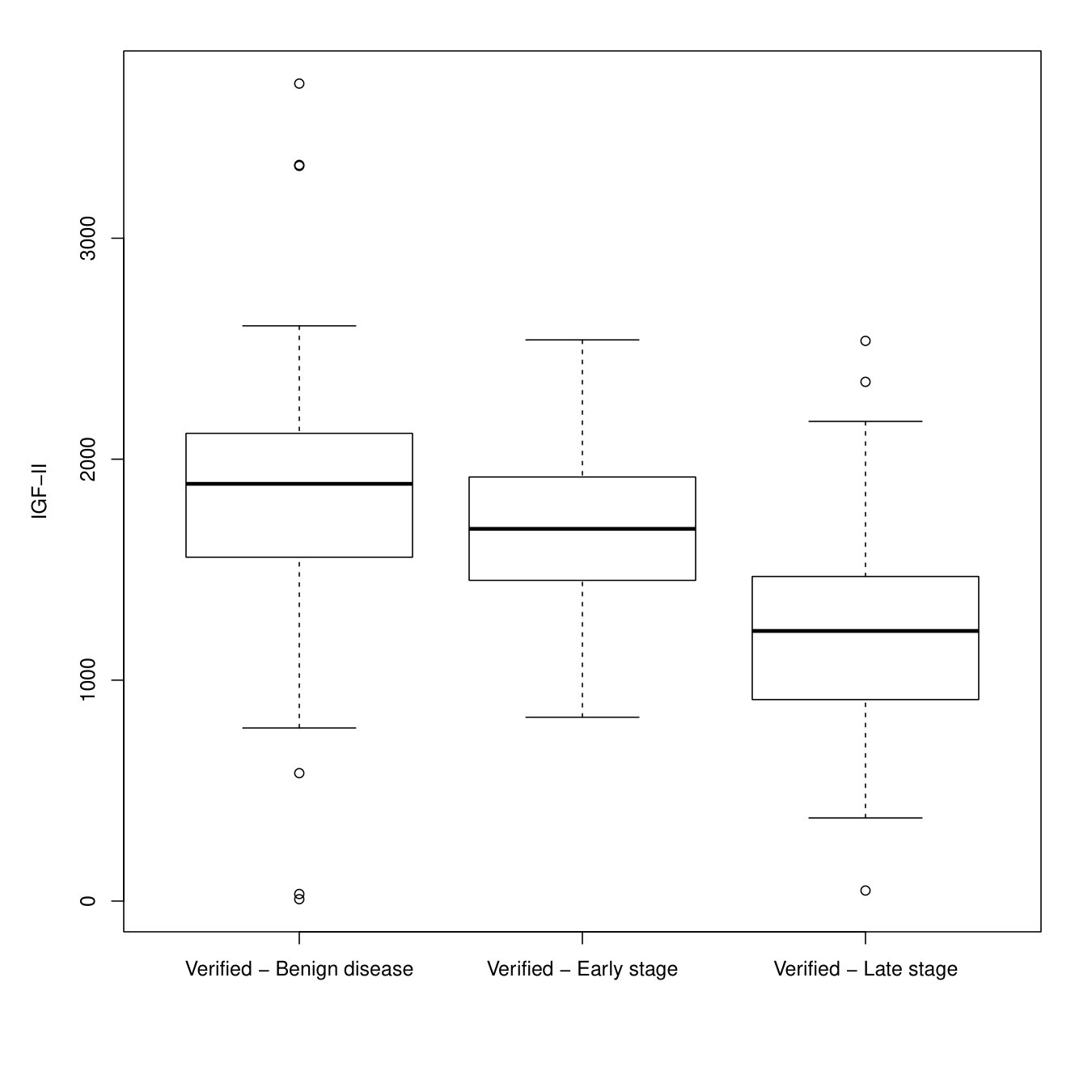 Figure 1
| MSEq | logLike | MSEq | logLike | MSEq | logLike | ||
| Scenario I | 2.081 | 0.750 | 1.992 | 1.189 | 2.274 | 1.806 | |
| 0.595 | 0.782 | 0.550 | 0.658 | 0.491 | 0.546 | ||
| 1.281 | 1.271 | 1.255 | 1.236 | 1.230 | 1.217 | ||
| 1.870 | 0.127 | 1.919 | 0.943 | 2.192 | 1.763 | ||
| 0.132 | 0.122 | 0.341 | 0.435 | 0.902 | 0.867 | ||
| FI | 0.775 | 0.761 | 0.776 | 0.771 | 0.784 | 0.783 | |
| MSI | 0.772 | 0.757 | 0.774 | 0.769 | 0.783 | 0.783 | |
| IPW | 0.778 | 0.765 | 0.776 | 0.770 | 0.783 | 0.782 | |
| PDR | 0.773 | 0.757 | 0.773 | 0.765 | 0.781 | 0.782 | |
| Scenario II | 3.154 | 5.071 | 2.119 | 5.217 | 1.553 | 4.011 | |
| 1.108 | 1.870 | 1.078 | 1.452 | 1.039 | 1.154 | ||
| 4.131 | 5.173 | 3.115 | 5.721 | 2.549 | 4.895 | ||
| 0.580 | 4.365 | 0.899 | 4.757 | 1.274 | 3.913 | ||
| FI | 0.844 | 0.799 | 0.845 | 0.822 | 0.843 | 0.835 | |
| MSI | 0.841 | 0.795 | 0.843 | 0.820 | 0.841 | 0.833 | |
| IPW | 0.841 | 0.822 | 0.842 | 0.829 | 0.841 | 0.836 | |
| PDR | 0.839 | 0.801 | 0.842 | 0.825 | 0.841 | 0.835 | |
| Bias(%) | MCSD | ASD | CP.Asy(%) | |
|---|---|---|---|---|
| FI | 0.6 | 0.070 | 0.075 | 95.8 |
| MSI | 0.6 | 0.070 | 0.075 | 95.8 |
| IPW | 0.1 | 0.074 | 0.069 | 93.2 |
| PDR | 0.6 | 0.070 | 0.075 | 95.8 |
| Scenario II: VUS = 0.843 | Scenario III: VUS = 0.457 | ||||||||||||
| Bias | MCSD | ASD | BSD | CP.Asy | CP.Bst | Bias | MCSD | ASD | BSD | CP.Asy | CP.Bst | ||
| FI | 0.2 | 0.054 | 0.055 | 0.057 | 88.9 | 92.2 | 1.4 | 0.070 | 0.144 | 0.075 | 96.8 | 94.5 | |
| MSI | 0.3 | 0.055 | 0.072 | 0.059 | 90.0 | 92.8 | 1.4 | 0.070 | 0.144 | 0.075 | 96.9 | 94.5 | |
| IPW | 0.3 | 0.059 | 0.064 | 0.061 | 88.9 | 91.3 | 0.6 | 0.083 | 0.083 | 0.087 | 93.8 | 94.3 | |
| PDR | 0.4 | 0.061 | 0.088 | 0.073 | 89.1 | 92.8 | 1.4 | 0.070 | 0.144 | 0.075 | 96.9 | 94.5 | |
| FI | 0.3 | 0.041 | 0.038 | – | 91.0 | – | 0.1 | 0.052 | 0.063 | – | 96.1 | – | |
| MSI | 0.0 | 0.042 | 0.040 | – | 92.3 | – | 0.1 | 0.052 | 0.062 | – | 96.1 | – | |
| IPW | 0.0 | 0.044 | 0.045 | – | 91.6 | – | 0.2 | 0.063 | 0.064 | – | 94.5 | – | |
| PDR | 0.1 | 0.044 | 0.049 | – | 91.2 | – | 0.1 | 0.052 | 0.063 | – | 96.2 | – | |
| FI | 0.0 | 0.028 | 0.026 | – | 92.5 | – | 0.8 | 0.037 | 0.040 | – | 95.6 | – | |
| MSI | 0.2 | 0.028 | 0.028 | – | 93.5 | – | 0.8 | 0.037 | 0.039 | – | 95.6 | – | |
| IPW | 0.2 | 0.030 | 0.029 | – | 93.0 | – | 0.5 | 0.043 | 0.045 | – | 95.3 | – | |
| PDR | 0.2 | 0.030 | 0.028 | – | 92.3 | – | 0.8 | 0.036 | 0.039 | – | 95.7 | – | |
| FI | 0.1 | 0.019 | 0.019 | – | 95.5 | – | 0.2 | 0.025 | 0.029 | – | 95.6 | – | |
| MSI | 0.0 | 0.019 | 0.020 | – | 95.8 | – | 0.2 | 0.025 | 0.029 | – | 95.5 | – | |
| IPW | 0.0 | 0.020 | 0.021 | – | 95.4 | – | 0.0 | 0.031 | 0.032 | – | 95.6 | – | |
| PDR | 0.0 | 0.020 | 0.020 | – | 94.8 | – | 0.2 | 0.025 | 0.029 | – | 95.5 | – | |
| Scenario IV: VUS = 0.843 | Scenario V: VUS = 0.74 | Scenario VI: VUS = 0.728 | |||||||||||
| Bias | MCSD | ASD | CP | Bias | MCSD | ASD | CP | Bias | MCSD | ASD | CP | ||
| FI | 0.8 | 0.059 | 0.055 | 89.9 | 3.6 | 0.090 | 0.063 | 89.6 | 5.2 | 0.081 | 0.068 | 90.7 | |
| MSI | 1.1 | 0.059 | 0.060 | 91.4 | 3.7 | 0.090 | 0.062 | 89.6 | 5.4 | 0.082 | 0.073 | 91.8 | |
| IPW | 0.1 | 0.064 | 0.063 | 88.9 | 2.2 | 0.070 | 0.066 | 95.4 | 5.5 | 0.083 | 0.071 | 91.1 | |
| PDR | 1.1 | 0.067 | 0.066 | 90.3 | 3.4 | 0.091 | 0.079 | 90.9 | 3.7 | 0.097 | 0.074 | 91.2 | |
| FI | 0.7 | 0.044 | 0.041 | 92.8 | 3.6 | 0.081 | 0.046 | 89.7 | 5.2 | 0.067 | 0.049 | 87.8 | |
| MSI | 1.0 | 0.044 | 0.041 | 93.8 | 3.7 | 0.081 | 0.045 | 89.2 | 5.4 | 0.068 | 0.055 | 90.3 | |
| IPW | 0.1 | 0.050 | 0.050 | 91.7 | 2.2 | 0.059 | 0.055 | 94.8 | 5.5 | 0.065 | 0.060 | 90.0 | |
| PDR | 1.1 | 0.051 | 0.051 | 92.3 | 3.4 | 0.083 | 0.054 | 90.4 | 3.7 | 0.068 | 0.056 | 90.7 | |
| FI | 0.9 | 0.031 | 0.028 | 92.7 | 1.8 | 0.050 | 0.032 | 94.4 | 5.0 | 0.047 | 0.036 | 81.9 | |
| MSI | 1.1 | 0.031 | 0.030 | 94.9 | 1.8 | 0.050 | 0.031 | 93.6 | 5.2 | 0.047 | 0.040 | 87.2 | |
| IPW | 0.1 | 0.034 | 0.032 | 91.7 | 1.3 | 0.039 | 0.045 | 97.1 | 5.4 | 0.049 | 0.040 | 85.0 | |
| PDR | 1.1 | 0.036 | 0.033 | 92.9 | 1.7 | 0.053 | 0.036 | 94.1 | 3.4 | 0.048 | 0.035 | 87.5 | |
| FI | 0.8 | 0.020 | 0.020 | 94.1 | 1.1 | 0.023 | 0.022 | 96.2 | 5.2 | 0.031 | 0.025 | 69.1 | |
| MSI | 0.9 | 0.020 | 0.021 | 95.1 | 1.1 | 0.023 | 0.021 | 94.9 | 5.3 | 0.031 | 0.029 | 78.0 | |
| IPW | 0.2 | 0.022 | 0.023 | 93.9 | 1.0 | 0.024 | 0.035 | 97.5 | 5.1 | 0.034 | 0.029 | 74.8 | |
| PDR | 0.8 | 0.023 | 0.023 | 95.4 | 0.9 | 0.028 | 0.024 | 95.1 | 3.2 | 0.032 | 0.025 | 82.0 | |
| Disease model | ||||||
| Benign disease | Early stage | |||||
| Est. | SE | -value | Est. | SE | -value | |
| Intercept | 1.832 | 0.786 | 0.020 | 0.528 | 0.218 | 0.015 |
| 0.922 | 0.204 | 0.001 | 0.880 | 0.205 | 0.001 | |
| 1.289 | 0.444 | 0.004 | 0.625 | 0.168 | 0.001 | |
| 17.131 | 4.325 | 0.001 | 0.026 | 0.141 | 0.852 | |
| Verification model | ||||||
| Logit link | Probit link | |||||
| Est. | SE | -value | Est. | SE | -value | |
| Intercept | 6.186 | 1.455 | 0.001 | 2.966 | 0.621 | 0.001 |
| 1.338 | 0.376 | 0.001 | 0.659 | 0.162 | 0.001 | |
| 5.733 | 1.501 | 0.001 | 2.649 | 0.639 | 0.001 | |
| 4.207 | 0.961 | 0.001 | 1.899 | 0.631 | 0.003 | |
| bias–corrected VUS | ||||||
| Logit link | Probit link | |||||
| Est. | SE | 95% CI | Est. | SE | 95% CI | |
| FI | 0.317 | 0.025 | 0.317 | 0.025 | ||
| MSI | 0.343 | 0.028 | 0.343 | 0.028 | ||
| IPW | 0.243 | 0.087 | 0.299 | 0.056 | ||
| PDR | 0.342 | 0.027 | 0.341 | 0.030 | ||
Peer Reviews
No public reviews on file for this paper yet. If you reviewed it on a platform where reviews are public (OpenReview, ICLR, NeurIPS, ICML), you can paste yours below so the community can read it here.
Videos
No videos yet. Explain this paper in a talk, walkthrough, or lecture? Add one.
Taxonomy
TopicsStatistical Methods in Clinical Trials · Statistical Methods and Inference · Statistical Methods and Bayesian Inference
Improving estimation of the volume under the ROC surface when data are missing not at random
Duc-Khanh To [email protected] Department of Statistical Sciences, University of Padova,
Gianfranco Adimari [email protected] Department of Statistical Sciences, University of Padova,
Monica Chiogna [email protected] Department of Statistical Sciences “Paolo Fortunati”, University of Bologna,
ABSTRACT
In this paper, we propose a mean score equation-based approach to estimate the the volume under the receiving operating characteristic (ROC) surface (VUS) of a diagnostic test, under nonignorable (NI) verification bias. The proposed approach involves a parametric regression model for the verification process, which accommodates for possible NI missingness in the disease status of sample subjects, and may use instrumental variables, which help avoid possible identifiability problems. In order to solve the mean score equation derived by the chosen verification model, we preliminarily need to estimate the parameters of a model for the disease process, but its specification is required only for verified subjects under study. Then, by using the estimated verification and disease probabilities, we obtain four verification bias-corrected VUS estimators, which are alternative to those recently proposed by To Duc et al., (2019), based on a full likelihood approach. Consistency and asymptotic normality of the new estimators are established. Simulation experiments are conducted to evaluate their finite sample performances, and an application to a dataset from a research on epithelial ovarian cancer is presented.
Key words: Diagnostic test; Instrumental variable; Mean score equation; Nonignorable missing data mechanism; ROC analysis; Verification bias.
1 Introduction and background
The evaluation of the accuracy of diagnostic tests (or biomarkers) is an increasingly relevant issue in modern medicine. Usually, this issue is solved by means of a receiver operating characteristic (ROC) analysis. In particular, the volume under the ROC surface (VUS) is often used for measuring the overall accuracy of a diagnostic test when the possible disease status belongs to one of three ordered categories. Under correct ordering, values of VUS vary from 1/6, suggesting that the test is no better than chance alone, to 1, that implies a perfect test, i.e. a test that perfectly discriminates among the three categories (Scurfield,, 1996).
In medical studies, the VUS of a new test is typically estimated through a sample of measurements obtained by some suitable sample of patients, for which the true disease status is assessed by means of a gold standard (GS) test. However, in many cases, due to the expensiveness and/or invasiveness of the GS test, only a subset of patients undergoes disease verification. In such situations, statistical inference based only on verified subjects is typically biased. This bias is known as verification bias.
In order to correct for verification bias, the researchers must formulate some assumptions about the selection mechanism for the disease verification. When the decision to send a subject to verification may be directly based on the presumed subject’s disease status, or, more generally, the selection mechanism may depend on some unobserved covariates related to disease, the missing data mechanism is called nonignorable (NI).
Generally speaking, NI data missingness is a challenge for inference, and, specifically, the issue of correcting for NI verification bias in ROC surface analysis is still scarcely considered in the statistical literature. To the best of our knowledge, only Zhang and Alonzo, (2018) and To Duc et al., (2019) gave a contribution in this direction. In particular, To Duc et al., (2019) extended the model discussed in Liu and Zhou, (2010) to match the case of three-category disease status, and proposed a likelihood-based approach to derive four bias–corrected estimators of the VUS, namely, full imputation (FI), mean score imputation (MSI), inverse probability weighting (IPW) and pseudo doubly robust (PDR) estimators.
Suppose we need to evaluate the predictive ability of a new continuous diagnostic test in a context where the disease status of a patient can be described by three ordered categories, “non–diseased”, “intermediate” and “diseased”, say. Consider a sample of subjects and let , and denote the test result, the disease status and a vector of covariates for each subject, respectively. Hereafter, we assume, without loss of generality, that test values are positively associated with the severity degree of the disease. The disease status can be modeled as a trinomial random vector , such that is a Bernoulli random variable having mean where . Hence, represents the probability that a generic subject, classified according to its disease status, belong to the class . The accuracy of is measured by its VUS, which is defined as
[TABLE]
where the indices , , refer to three different subjects, and is the indicator function (Nakas and Yiannoutsos,, 2004). When the disease status is available for all subjects, a natural nonparametric estimator of is given by
[TABLE]
Suppose now that the disease status is missing for a subset of patients in the study. Let be the verification status for the -th subject in study, that is if is observed and otherwise. To account for a possible nonignorable missing data mechanism for the disease status, To Duc et al., (2019) considered the verification model
[TABLE]
where the parameters and describe the type of missingness mechanism. In particular, the missing data mechanism is ignorable (MAR) if ; NI, otherwise. Following Liu and Zhou, (2010), to estimate the parameter in the verification model (1.3), To Duc et al., (2019) proposed to use a likelihood-based approach. Specifically, the authors assumed that the disease process follows a multinomial logistic model for the whole sample, i.e.,
[TABLE]
where . Then, they jointly considered the verification model (1.3) and the disease model (1.4) to construct the (observed) log-likelihood function, say, where is the vector of parameters of the disease model. The authors proved that the joint model based on (1.3) and (1.4) is identifiable. Then, the maximum likelihood estimator (MLE) of can be obtained by maximizing or solving the corresponding score equation. Based on imputation and re-weighting methods, four estimators for each disease status can be obtained: FI, with ; MSI, with , where ; IPW, with and PDR, with , with . Therefore, bias-corrected VUS estimators are derived by using quantities in (1.2), i.e.,
[TABLE]
Here, the symbol stands for type of estimator, i.e., FI, MSI, IPW and PDR.
Despite its usefulness, the above reviewed approach presents some limitations. Firstly, it is scarcely flexible, since identifiability is proven only for the specific parametric assumptions about the verification and the disease processes. Secondly, because of NI missigness, it does not allow a statistical check of appropriateness of such assumptions (see also Riddles et al.,, 2016, Morikawa et al.,, 2017 and Yu et al.,, 2018). Finally, as pointed out by the authors themselves, MLE of ignorable/nonignorable parameters and are typically highly biased, in cases of moderate or even high sample sizes.
In the present paper, we try to overcome such limitations. More precisely, here we consider the mean score function as a tool to estimate the parameters in the verification model, and avoid identifiability problems by resorting to the introduction of instrumental variables (Wang et al.,, 2014; Riddles et al.,, 2016). As we show in what follows, in order to solve the mean score equation derived by the chosen verification model, we preliminarily need to estimate the parameters of a model for the disease process, but its specification is required only for verified subjects. Thus, the new proposed approach essentially avoids the specification of a parametric regression model for the disease status of the whole sample, and presents the advantage that it allows a statistical evaluation, based on the available sample data, of the adequacy of the required conditional (to ) disease model. Furthermore, as confirmed by our simulation experiments, the reduction in complexity of the adopted model translates into a greater stability of estimates of the parameters.
Based on the new approach, we provide four new VUS estimators (FI, MSI, IPW and PDR), which accommodate for nonignorable missingness of the disease status. We prove consistency and asymptotic normality of the proposed estimators, and also provide estimators of their variances.
The paper is organised as follows. In Section 2, we present the proposed approach, and give the new bias–corrected VUS estimators, for which, in Section 3, we discuss the asymptotic behaviour. In Section 4, we present the results of the simulation study, and in Section 5 we give an illustrative application. Section 6 contains some final remarks. Some technical details can be found in Appendix.
2 The proposal
It is worth noting that MLE of , on which estimators (1.5) ultimately rely, could be also obtained as solution of the so-called mean score equation (Louis,, 1982; Kim and Shao,, 2013; Riddles et al.,, 2016). Let and denote the score functions derived from the verification model (1.3) and from the disease model (1.4), respectively. For the joint model, the mean score function is (Kim and Shao,, 2013), with
[TABLE]
where and denote the standard contributions to and , respectively. Terms , represent the contribution to the scores, arising from unverified subjects.
Hereafter, we consider an alternative estimation procedure which solves the mean score equation derived from the verification model only, and uses instrumental variables. To this aim, we assume that the vector of covariates can be decomposed as such that the verification status does not depend on given , , and . Variable is known as instrumental variable and helps to make the verification model identifiable (see Wang et al.,, 2014 and Riddles et al.,, 2016) without further assumptions on the disease model. By using the instrumental variable , we can reduce the verification model (1.3) to
[TABLE]
where . Then, MLE estimate of can be obtained by solving the mean score equation where
[TABLE]
with
[TABLE]
for and
[TABLE]
Let denote for and . By an application of Bayes’ rule (see Appendix A), it can be shown that
[TABLE]
Hence, the mean score function (2.3) depends on the disease probabilities for verified units only. If (just to keep the parallel with the proposal in To Duc et al., (2019)) we use a multinomial logistic regression model for the conditional disease probabilities , i.e.,
[TABLE]
, the functions depend also on , and the expressions in (2.5) become
[TABLE]
By using (2.4) and (2.7), the mean score function (2.3) can be rewritten as
[TABLE]
Then, once an estimate is available, we can get an empirical form of the mean score function (2.3), say . The empirical mean score equation can be solved to obtain an estimate of .
Observe that would be the MLE estimate only if was solution of equation (2.1). It should be noted, however, that in our simplified approach, is the solution of a score equation that depends on the parametric model specification for the conditional (to ) disease process. The verification mechanism may be modelled by means of a generalised linear regression model for binary data with a fixed link function (e.g., logistic, probit, log-log or complementary log-log). Whichever choice is taken, identifiability of the model holds thanks to the use of instrumental variables. In what follows, for the purposes of presentation, we adopt a standard logistic model for the verification process, and a multinomial logistic model for the conditional (to verification) disease process, a solution that also allow to keep the parallel with the approach in To Duc et al., (2019).
Let , with , denote the estimating function for based on the verified units in the sample. Since our empirical mean score equation is a specific case of a more general one discussed by Riddles et al., (2016), it follows that, under certain regularity conditions given in Appendix B, and are consistent and asymptotically normal estimators (see Theorem 1 in Riddles et al.,, 2016).
In order to obtain four bias-corrected VUS estimators (FI, MSI, IPW and PDR), we follow the arguments in To Duc et al., (2019), starting by the fact that
[TABLE]
and considering the quantities
[TABLE]
[TABLE]
[TABLE]
in which we stressed the fact that the probabilities of selection for verification depend on . Plugging in the above expressions the estimates and , yields the estimates , , and . Then, the bias-corrected VUS estimators are obtained by replacing each disease status in (1.2) with the new estimates , where the symbol indicates, again, the kind of estimator, i.e., FI, MSI, IPW and PDR.
Note that, the parameters of the verification model (2.2) and of the conditional (to ) disease model (2.6) are estimated separately (see the estimation process in Appendix C). However, the accuracy of the estimates in the verification model (2.2) may suffer from possible fitting’s problems in the disease model (2.6), because the empirical mean score equation uses . On the other hand, the estimates also may be affected by possible poor accuracy in the estimation of , or . Ultimately, the fact that the proposed method is a parametric method has as a consequence that it could produce VUS estimates even strongly influenced by incorrect specifications of the involved models.
3 Asymptotic behaviour
As for the estimators discussed in To Duc et al., (2019), the new proposed VUS estimators can be found as solutions of appropriate estimating equations, solved along with the score equations and the empirical mean score equation . The estimating functions for FI, MSI, IPW and PDR estimators have generic term (corresponding to a generic triplet of sample units), respectively,
[TABLE]
for , and . In the following, we will use the general notation , where stands for FI, MSI, IPW and PDR, and denote by the corresponding new VUS estimator. Moreover, let , and be the true parameter values. We assume that
- (C1)
the U–process, , is stochastically equicontinuous, where
[TABLE]
and
[TABLE] 2. (C2)
is differentiable in , and \dfrac{\partial e_{*}(\mu,\boldsymbol{\eta}_{0},\boldsymbol{\gamma}_{0})}{\partial\mu}\Bigg{|}_{\mu=\mu_{0}}\neq 0; 3. (C3)
and converge uniformly (in probability) to and , respectively.
Let , , and .
Theorem 3.1**.**
Suppose that conditions (C1)–(C3), and (D1)–(D9) in Appendix B, hold. Then, under the verification model (2.2) and the (conditional) disease model (2.6), is consistent and asymptotically normal, i.e.,
[TABLE]
where and
[TABLE]
Proof.
(sketch). Under the verification model (2.2) and the disease model (2.6), we can show that quantities have 0 expectation. Then, the consistency of can be proven by arguments similar to those used in Theorem 1 of To Duc et al., (2019). As for the asymptotic normality, we follow the steps in the proof of Theorem 2 in To Duc et al., (2019). In particular, using also equation (B.1), since , we can write
[TABLE]
An application of a standard result about the limit distribution of U-statistics (van der Vaart,, 2000), yields to
[TABLE]
This, together with the fact that
[TABLE]
and equation (B.1), show that (3.1) is equivalent to
[TABLE]
Then, we have that
[TABLE]
and the asymptotic normality of follows by the Central Limit Theorem. ∎
The asymptotic variances can be consistently estimated by
[TABLE]
where
[TABLE]
and
[TABLE]
Clearly, alternative approaches to estimate the variance of the proposed VUS estimators are possible. For instance, one may resort to the classical bootstrap method.
4 Simulation study
In order to compare the proposed mean score equation-based approach with the fully likelihood-based method in (To Duc et al.,, 2019) and to evaluate the performance of the new bias-corrected VUS estimators, we carry out several simulation experiments. The number of replications is 1000 in each experiment, and the considered sample sizes are and .
4.1 Simulation setup
With regard to data generation, we consider the following six different scenarios:
- I.
For each unit, the test result and a covariate are generated by the model
[TABLE]
The disease status is generated by the following multinomial logistic model:
[TABLE]
The verification status is simulated by the following logistic model
[TABLE]
Under this setting, the verification rate is roughly 0.57 and the true VUS is 0.791. This setting is the same as Scenario I in To Duc et al., (2019). 2. II.
For each unit, the disease status is generated from a multinomial distribution with , and (recall that ). The test results and a covariate are generated as and , while the verification status is simulated through the model
[TABLE]
The verification rate is roughly 0.44 and the true VUS is 0.843. 3. III.
The disease status is generated as in scenario I. The test results and a covariate are generated as and , for . A second covariate is simulated as , and . The true VUS is 0.457. The verification status is simulated by a probit model
[TABLE]
where denotes cumulative distribution function of a standard normal. In this case, the verification rate is roughly 0.47. 4. IV.
The disease status , the test result and a covariate are generated in the same way as in scenario II. The verification status is simulated through the model
[TABLE]
The verification rate is roughly 0.42, and the true VUS still is 0.843. 5. V.
We generate the test result , two covariates and . The disease status is generated by using the multinomial logistic model
[TABLE]
The verification status is simulated by the following model:
[TABLE]
In this scenario, the verification rate is roughly . The true VUS value is . 6. VI.
We generate the test result , and two covariates as in scenario IV. The disease status is generated by using the multinomial logistic model
[TABLE]
The verification status is simulated by the following model:
[TABLE]
The verification rate is roughly , and the true VUS value is .
Scenarios I and II aim to compare the discussed mean score equation-based approach with the fully likelihood-based one, in terms of accuracy of parameter estimators in the verification model, and VUS estimators. As pointed out above, scenario I is identical to Scenario I in To Duc et al., (2019) and does not involve instrumental variables. On the contrary, in scenario II the covariate plays the role of instrumental variable. Moreover, scenarios II to VI aim to assess the finite-sample behavior of new proposed bias-corrected VUS estimators. In particular, as explained below, scenarios IV, V and VI serve to evaluate the effects on the estimators of some types of misspecifications in the working models.
By applying the Bayes’ rule, for all considered scenarios, the true conditional (to ) disease process takes the following form:
[TABLE]
where is simply the covariate in the scenarios I, II, IV and V, in scenarios III and VI and , and denote , and , respectively. Clearly, in practice this is a multinomial logistic model with unknown offset terms (intercepts).
In making simulations, when considering the new mean score equation-based approach, we fit the the conditional disease model as a multinomial logistic one, i.e., we specify the working conditional disease model as follows:
[TABLE]
where for scenarios I, II and IV, for scenarios III and V and for scenario VI. As for the verification model, in the estimation procedure we use the correct logistic model in scenarios I, II, III and VI, while in scenarios IV we use a logistic models involving only , and in scenario V we use a probit model involving only and the covariate Therefore, the working models are correctly specified in scenarios I, II and III, while they present various types of misspecification in scenarios IV, V and VI. More precisely: in scenario IV, we omit the covariate in the verification model and use it as instrumental variable; in scenario V, we omit the covariate in the verification model, use it as instrumental variable and incorrectly define the model (probit instead of logit); in scenario VI, we use instead of and omit the interaction term in the conditional disease model. Finally, as for the fully likelihood-based approach, in scenarios I and II, the working (unconditional) disease model and the working verification model are both correctly specified.
4.2 Computational aspects
In order to obtain the new VUS estimates, in our simulation we need to solve, at each replication, the score equation , and then the empirical mean score equation . The first equation refers to the conditional (to ) disease model and, since we work with a multinomial logistic model in all scenarios, we resort to the routine multinom() (of R package nnet) to solve it. Given , the empirical mean score equation could be solved in by using some numeric algorithm, such the ones deployed in the R routine nleqslv(). However, numerical algorithms for solving equations are often poorly stable and reliable, or, better, are less reliable than optimization algorithms. Therefore, in order to obtain , we minimize the squared Euclidean norm of , i.e., . The optimization is performed by using the L-BFGS-B algorithm supplied in the R routine optim().
4.3 Results
Simulation results are given in tables 1-3. Table 1 refers to the comparison between the mean score equation-based approach (MSEq) and the fully likelihood-based approach (logLike). For three different sample sizes, i.e., 150, 250 and 500, the table provides Monte Carlo means for the estimators of the parameters in the verification model, together with Monte Carlo means for the four (FI, MSI, IPW and PDR) VUS estimators, for scenarios I and II. Recall that, in such scenarios, the considered working models are correctly specified. The results clearly show that the new approach achieves better performance, providing less biased estimators, already at the smallest sample size.
Results in Table 2 allow us to evaluate the behavior of the proposed VUS estimators, and of the corresponding variance estimators based on (3.2), when the considered working models are correctly specified. For both scenarios II and III and four different sample sizes (150, 250, 500 and 1000), the table contains Monte Carlo relative biases, Monte Carlo standard deviations and (means of) estimated standard deviations based on (3.2), for the new VUS estimators. The table also provides the empirical coverages of the 95% confidence intervals for the VUS, obtained through the normal approximation approach applied to each estimator and the use of the corresponding variance estimator (3.2).
Overall, Table 2 shows that the proposed approach provides satisfactory results in terms of relative bias and coverage probability when the verification models are correctly specified. At the smallest sample size, the larger absolute relative bias is equal to (scenario III). As expected, when the sample size increases, the relative bias of the VUS estimators decreases, becoming negligible for . Moreover, especially for scenario III (in which the verification process follows a probit model), in case of smallest sample size, , the (means of) estimated standard deviations based on (3.2) still seem to be affected by a poor accuracy in the estimation of the parameters in the working models. However, in similar cases, as shown in the table, more accurate estimates of standard deviations can be obtained via bootstrap. Bootstrap estimates also improve empirical coverage probabilities of confidence intervals, when used within the normal approximation approach (see also the results for scenario II).
We emphasize that, when working models are correctly specified, low-accuracy problems can be related to low verification rates. For example, in scenario III the verification rate is 0.47. If we change the verification process and use the following model to simulate values:
[TABLE]
the verification rate becomes roughly 0.72, and the corresponding simulation results (for and 1000 replications), given below,
are clearly better than those in Table 2.
[FIGURE:]
Table 3 presents the simulation results for scenarios IV-VI, in which the working models are, in various ways, misspecified. Again, for each scenario and four different sample sizes, the table gives Monte Carlo relative bias, Monte Carlo standard deviations and (means of) estimated standard deviations based on (3.2), for the new VUS estimators. The table also provides the empirical coverages of the 95% confidence intervals for the VUS, obtained through the normal approximation approach applied to each estimator and the use of the corresponding variance estimator (3.2).
In the considered scenarios, all proposed VUS estimators appear to be biased, even when the sample size increases. However, simulation results appear to stay on acceptable levels (the relative biases are not too large and the coverage probabilities are close to 95%) in scenarios IV and V, i.e., when the misspecification follows by the omission of a variable and/or a wrong choice of the link function in the working generalized linear model for the verification process. Clearly, due to the strong deviation between the working conditional disease model and the true one, the results are significantly worse in the scenario VI. Anyway, variance estimators (3.2) seem relatively more robust with respect to the considered misspecifications in the working models.
[FIGURE:]
5 Application
We illustrate an application of our method by using data from the Pre-PLCO Phase II Dataset, from the SPORE/Early Detection Network/Prostate, Lung, Colon, and Ovarian Cancer Study. The study protocol and the data are publicly available at the address 111http://edrn.nci.nih.gov/protocols/119-spore-edrn-pre-plco-ovarian-phase-ii-validation. In this study, several serum protein biomarkers are evaluated in terms of their ability to correctly classify possible epithelial ovarian cancer (EOC) cases into benign disease, early stage (I-II) and late stage (III-IV). Among such biomarkers, we are interested in insulin-like growth factor-II (IGF-II), previously studied in Mor et al., (2005) and Visintin et al., (2008) to distinguish non-diseased from cancer cases (early stage and the late stage). The data we consider refer to 156 patients with benign disease, 71 patients with early stage, and 82 with late stage. Moreover, the data present 87 unverified units; therefore, only 78% of patients receive the assessment of their true disease status.
The boxplots for the IGF-II values, stratified by the disease status and based on the verified units only, are presented in Figure 1, which show that lower values of IGF-II are associated with higher severity of disease; thus, in our analysis, we consider minus the values of the IGF-II as test values. Moreover, we consider two other serum proteins, i.e., HE4 and CA125, as covariates.
Our goal is to estimate the VUS for the IGF-II biomarker. In the analysis, we standardize the values of IGF-II, HE4 and CA125, and below, for convenience, denote them as , and , respectively. We also let and to be the variables corresponding to benign disease and early stage, respectively.
We fit the conditional (to ) disease model by using a multinomial logistic regression model with , and as predictors and late stage as reference level. As for the verification model, we consider a logistic model and a probit model, with only as a predictor; hence, and are used as instrumental variables. The estimated parameters, estimated standard errors and corresponding -values for the significance test for coefficients in the models are given in Table 4. The -values refer to the Wald-type statistics, which use results in (B.4). The resulting -values for ignorable/nonignorable coefficients in both models (logistic and probit), indicate that, in such case, the missing data mechanism is nonignorable.
Table 4 also provides the four bias-corrected VUS estimates, along with the standard errors and 95% confidence intervals (CI), constructed using normal approximation and (3.2). The Naïve VUS estimate, calculated from verified subjects only, is 0.460 with standard error 0.035 and 95% CI . Therefore, all bias-corrected VUS estimates are significantly different to the Naïve one. Moreover, unlike the logistic model, the IPW estimate in probit model is comparable to the other VUS estimates. This may suggest that the probit link function is a good choice for the generalized regression model describing the verification process for these data.
Finally, we highlight the purely illustrative nature of this application and the fact that, in real applications, the approach proposed in this paper allows to evaluate the model chosen to describe the (conditional) disease process by diagnostic procedures and/or ad hoc statistical tests present in the litterature, as those, for instance, in Goeman and le Cessie, (2006) for the multinomial logistic regression model.
6 Conclusion
In this paper, we propose a mean score equation-based approach to estimate the volume under a ROC surface when the disease status is missing not at random. This approach can take advantage of the use of instrumental variables, which help avoid possible identifiability problems. We prove that our proposed bias–corrected VUS estimators are consistent and asymptotically normal.
Our method is essentially a parametric method, and requires the estimation of the parameters of a (parametric) model chosen to describe the conditional (to ) disease process, and then the solution of an empirical mean score equation resulting from a parametric model chosen for the verification process. The method may also be used in a semiparametric context, by resorting to a nonparametric regression approach to fit the conditional disease model, as in Morikawa et al., (2017). Clearly, this topic deserves further investigation.
Compared to the fully likelihood-based approach discussed in To Duc et al., (2019), the new method is simpler, and more flexible also thanks to the possible use of instrumental variables. Moreover, as our simulation results show, the new bias–corrected VUS estimators are generally more accurate with moderate sample sizes.
Resorting to instrumental variables may be necessary when relying on working models other than those, namely logistic and multinomial logistic, assumed by To Duc et al., (2019) to describe, respectively, the verification and disease process. In practice, however, the choice of variables that could play the role of instrumental variables is not trivial. With respect to this issue, we suggest a possible selection strategy that foresees three steps:
- (i)
choose a working model for the conditional (to ) disease process and select (by using a standard backward stepwise regression) a vector of covariates , statistically significant; 2. (ii)
choose a working model for the verification process and, given the estimate obtained in step (i), use, one at a time, the elements of , jointly with the test , to solve the resulting empirical mean score equation ; 3. (iii)
take as vector of instrumental variables, the vector consisting of the elements of resulting statistically non-significant at the previous step (ii).
Then, the final estimate is obtained by solving the empirical mean score equation based on and, when does not coincide with , the component of . This is also the selection strategy that we used in the illustrative application of Section 5.
Appendix A Conditional probabilities of disease for unverified subjects
Applying Bayes’ rule, we have
[TABLE]
for . Thus, we obtain the following ratios
[TABLE]
where
[TABLE]
with . These expressions are equivalent to the system of equations
[TABLE]
By using the fact that , from (A.1a), we obtain
[TABLE]
Substituting (A.2) into (A.1b), leads to the following equation
[TABLE]
After some algebra, we obtain that is equal to
[TABLE]
and then is
[TABLE]
In case of the logistic model (2.2), it is straightforward to show that
[TABLE]
Thus, we get the results in (2.5).
Appendix B Conditions for asymptotic normality of
Recall that , , and consider the conditions:
- (D1)
for given two values of the (instrumental) variable , and
[TABLE]
with ; 2. (D2)
is a continuous function of with first and second derivatives continuous in an open set containing as an interior point; 3. (D3)
the variables , , are independent and identically distributed; 4. (D4)
the parameter spaces for and for are compact and have finite dimension; 5. (D5)
is bounded away from 0. 6. (D6)
the MLE , say, is consistent and asymptotically normal; 7. (D7)
has a unique solution ; 8. (D8)
exists and is invertible; 9. (D9)
there exists a neighborhood of such that the quantiles , and have finite expectations, with .
By Theorem 1 in Riddles et al., (2016), under the regularity conditions (D1)–(D9), the solution of
[TABLE]
is a consistent estimator of , and satisfies
[TABLE]
Thus, by the Central Limit Theorem, is asymptotically normal. Moreover,
[TABLE]
where
[TABLE]
and
[TABLE]
where . Consistent estimators of and of can be obtained by
[TABLE]
with .
Appendix C Estimation Procedure
Modelling Verification Process
Modelling Disease Process for Verified Subjects (eventually using instrumental veriables)
Empirical Mean Score Equation
, , , ,
VUS-FI Estimator
VUS-MSI Estimator
VUS-PDR Estimator
VUS-IPW Estimator
The reference list from the paper itself. Each links out to its DOI / PubMed record.
- 1Goeman and le Cessie, (2006) Goeman, J. J. and le Cessie, S. (2006). A goodness-of-fit test for multinomial logistic regression. Biometrics , 62(4):980–985.
- 2Kim and Shao, (2013) Kim, J. K. and Shao, J. (2013). Statistical methods for handling incomplete data . Chapman and Hall/CRC.
- 3Liu and Zhou, (2010) Liu, D. and Zhou, X. H. (2010). A model for adjusting for nonignorable verification bias in estimation of the ROC curve and its area with likelihood–based approach. Biometrics , 66(4):1119–1128.
- 4Louis, (1982) Louis, T. A. (1982). Finding the observed information matrix when using the em algorithm. Journal of the Royal Statistical Society. Series B (Methodological) , 44(2):226–233.
- 5Mor et al., (2005) Mor, G., Visintin, I., Lai, Y., Zhao, H., Schwartz, P., Rutherford, T., Yue, L., Bray-Ward, P., and Ward, D. C. (2005). Serum protein markers for early detection of ovarian cancer. Proceedings of the National Academy of Sciences , 102(21):7677–7682.
- 6Morikawa et al., (2017) Morikawa, K., Kim, J. K., and Kano, Y. (2017). Semiparametric maximum likelihood estimation with data missing not at random. Canadian Journal of Statistics , 45(4):393–409.
- 7Nakas and Yiannoutsos, (2004) Nakas, C. T. and Yiannoutsos, C. T. (2004). Ordered multiple-class ROC analysis with continuous measurements. Statistics in Medicine , 23(22):3437–3449.
- 8Riddles et al., (2016) Riddles, M. K., Kim, J. K., and Im, J. (2016). A propensity-score-adjustment method for nonignorable nonresponse. Journal of Survey Statistics and Methodology , 4(2):215–245.