Passive viscoelastic response of striated muscles
Fabio Staniscia, Lev Truskinovsky

TL;DR
This paper develops a novel second-order rheological model for the passive viscoelastic response of striated muscles, incorporating long-range interactions and validated with frog muscle data.
Contribution
It introduces a new second-order continuum model for muscle mechanics derived from a stochastic micromodel, improving upon previous first-order approaches.
Findings
Model shows excellent agreement with experimental data
Second-order equation captures complex muscle behavior
Microscopic parameters accurately predict macroscopic response
Abstract
Muscle cells with sarcomeric structure exhibit highly nontrivial passive mechanical response. The difficulty of its continuum modeling is due to the presence of long-range interactions transmitted by extended protein skeleton. To build a rheological model for muscle 'material' we use a stochastic micromodel and derive a linear response theory for a half-sarcomere. Instead of the first order rheological equation, anticipated by A.V. Hill on the phenomenological grounds, we obtain a novel second order equation. We use the values of the microscopic parameters for frog muscles to show that the proposed rheological model is in excellent quantitative agreement with physiological experiments.
Click any figure to enlarge with its caption.
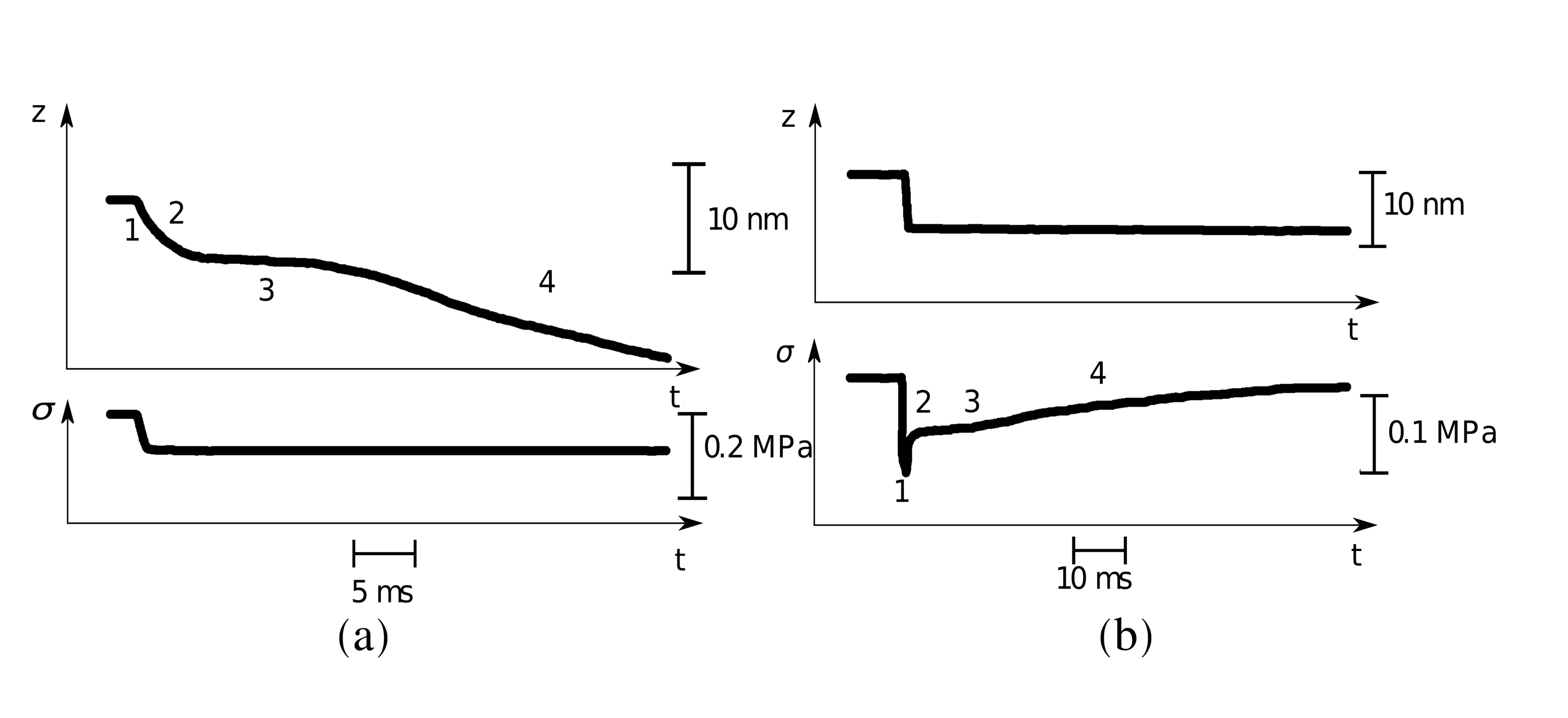 Figure 1
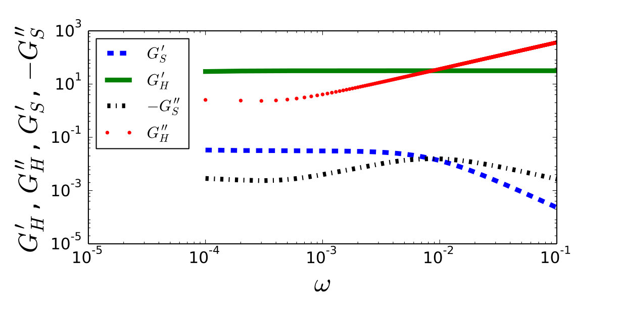 Figure 2
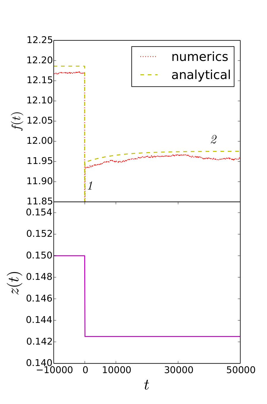 Figure 3
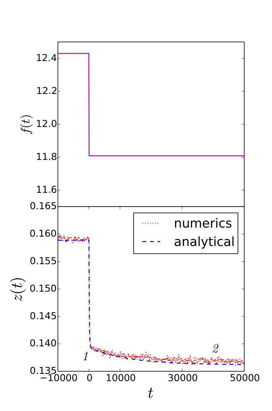 Figure 4
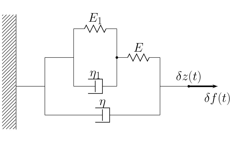 Figure 5
Peer Reviews
No public reviews on file for this paper yet. If you reviewed it on a platform where reviews are public (OpenReview, ICLR, NeurIPS, ICML), you can paste yours below so the community can read it here.
Videos
No videos yet. Explain this paper in a talk, walkthrough, or lecture? Add one.
Taxonomy
TopicsBlood properties and coagulation
Passive viscoelastic response of striated muscles
Fabio Staniscia
LMS, École polytechnique, 91128 Palaiseau Cedex, France
Lev Truskinovsky
PMMH, CNRS - UMR 7636 PSL-ESPCI, 10 Rue Vauquelin, 75005 Paris, France
Abstract
Muscle cells with sarcomeric structure exhibit highly nontrivial passive mechanical response. The difficulty of its continuum modeling is due to the presence of long-range interactions transmitted by extended protein skeleton. To build a rheological model for muscle ’material’ we use a stochastic micromodel and derive a linear response theory for a half-sarcomere. Instead of the first order rheological equation, anticipated by A.V. Hill on the phenomenological grounds, we obtain a novel second order equation. We use the values of the microscopic parameters for frog muscles to show that the proposed rheological model is in excellent quantitative agreement with physiological experiments.
pacs:
87.19.Ff, 46.35.+z, 87.15.A-, 87.85.jc
One of the simplest biological systems, that still defies the attempts to reproduce it artificially as a macroscopic material, is a striated muscle Kidambi et al. (2018). Its mechanical complexity is due to the presence of a large number of nonlinear, hierarchically organized microscopic sub-systems that are strongly coupled through long-range interactions Caruel and Truskinovsky (2018). This makes the task of reconstructing the macroscopic constitutive relations describing even its passive mechanical response rather challenging Caruel et al. (2019); Regazzoni et al. (2018).
A broadly used phenomenological theory of the passive visco-elastic response of striated muscles, proposed by A.V.Hill Hill (1938, 1949); Glantz (1974); Gerazov and Garner (2016), does not rely on coarse graining techniques DeVault and McLennan (1965); Bavaud (1987) and therefore does not offer a link between macro and micro parameters. Since Hill’s rheological relation involves a single characteristic time scale, it also does not capture the difference in the passive response exhibited by striated muscles abruptly loaded in soft (isotonic) and hard (isometric) loading devices Huxley and Simmons (1971); Reconditi et al. (2004).
A microscopically guided stochastic approach to muscle visco-elasticity was proposed by Huxley and Simmons Huxley and Simmons (1971); Eisenberg et al. (1980) who assumed that the individual force producing units (myosin cross-bridges) are stochastically independent. A mean-field interaction between the cross-bridges was incorporated in a closely related model by Shimizu Shimizu and Yamada (1972); Kometani and Shimizu (1975); Bonilla (1987); Frank (2004). The two approaches have been recently unified Marcucci and Truskinovsky (2010a, b); Caruel et al. (2013); Caruel and Truskinovsky (2018). In the present article we use this framework to rigorously derive from a micro-model a linear rheological response theory for a muscle half-sarcomere. Our analysis builds on the work of Shiino Shiino (1987) who obtained a similar linear response theory for the related model of Desai and Zwanzig Desai and Zwanzig (1978); Bonilla (1987); Frank (2004); other relevant out-of-equilibrium systems were studied in Patelli et al. (2012); Patelli and Ruffo (2014).
Our main result is the linear spring-dashpot scheme which reproduces adequately the mechanical behavior of a muscle fiber subjected to a time dependent perturbation. In contrast to the classical model of Hill Hill (1938, 1949), the proposed rheological equation contains not only the first but also the *second * time derivatives of the macroscopic displacement. We use the values of the microscopic parameters for frog muscles to show that our macroscopic model, which does not rely on any fitting parameters, is in excellent quantitative agreement with physiological experiment.
The model contains two time scales that can be associated with the transient stages of muscle response known as phases 1 and 2, see Fig. 1 and Huxley and Simmons (1971); Piazzesi et al. (2003); Decostre et al. (2005); Pia (2007), with both of them captured adequately by our rheological model. The presence of the two time scales reflects involvement of the two parallel passive processes: the (microscopic) conformational change in myosin heads and the macroscopic relaxation of the myofilaments in a viscous environment. The obtained linear rheological equation does not capture the collective barrier crossing which can be associated with the slower phase 3 explained in Caruel and Truskinovsky (2016, 2017, 2018); it also does not address the active phase 4, see Fig. 1.
We recall that striated muscle is a hierarchical chemo-mechanical system with the smallest scale represented by force generating half-sarcomeres Alberts et al. (2013); Caruel and Truskinovsky (2018). To reproduce the passive response of this molecular machine we use the simplest microscopic model developed in Marcucci and Truskinovsky (2010a, b); Caruel et al. (2013); Caruel and Truskinovsky (2016, 2017). We assume that behind the muscle power stroke, responsible for fast force recovery, is a double well potential of Landau type, , describing two conformational states of a cross-bridge Marcucci and Truskinovsky (2010a); it is known that myosin heads can be in other configurations Huxley (1974); Decostre et al. (2005); Caremani et al. (2013), so here we simplify the real physical picture Molloy et al. (1995); Reconditi et al. (2004). We also assume that the potential is asymmetric, which allows the system to generate (stall) force in the physiological regime of isometric contractions. While this asymmetry is maintained actively Sheshka et al. (2016), we can still interpret the short time response in such system as passive. The active response involving detachment of the cross-bridges becomes dominant at time-scales of the order of ms Howard (2001).
To define the dimensionless units we rescale the length by the size of the maximum working stroke , the energy by , where is the cross-bridge stiffness, and the time by the ratio of the cross-bridge drag coefficient and . To model a bundle of thick and thin filaments linked by cross-bridges and loaded with the force we use the dimensionless energy Caruel and Truskinovsky (2018)
[TABLE]
where the variables represent the configuration of individual cross bridges. The latter are elastically coupled through the cross-bridge stiffness to a collective variable representing an actin filament; the associated quadratic term in (1) represents mean field type interaction. The combined elasticity of actin and myosin filaments is described by the quadratic term coupling the variable and with the dimensionless coefficient representing the overall filamental stiffness, see Caruel and Truskinovsky (2018) for more details.
We assume that the meso-scopic collective variable relaxes instantaneously Huxley et al. (1994); Wakabayashi et al. (1994) and we can therefore eliminate such (Weiss-type) variable adiabatically. We obtain where we introduced notation Substituting the obtained expression for into (1) we obtain the redressed energy whose main feature vis-à-vis the model of Huxley and Simmons is the presence of all-to-all interaction between the cross-bridges expressed through the term , see also Desai and Zwanzig (1978); Shiino (1987).
Next we assume that the macro-variable is also deterministic, however now its dynamics is governed by the relaxation equation: where the superimposed dot denotes time derivative and is the dimensionless macroscopic friction coefficient obtained by normalizing the filamental drag coefficient by the myosin head drag coefficient . We can rewrite this equation as
[TABLE]
The time scale will then characterize the evolution of the macro-variable .
In the evolution of the micro-variables we need to account for the thermal noise: where and . Here we introduced the inverse dimensionless temperature . Under the assumption that is large, the single particle probability density can be found from the nonlinear Fokker-Planck equation Desai and Zwanzig (1978); Shiino (1987); Frank (2005)
[TABLE]
where we use approximation . The stationary solution of (3) is , where
[TABLE]
is an effective double well potential and is a normalization constant Caruel and Truskinovsky (2018). In (4) we must use the self-consistence condition ; such closure can be justified rigorously in the thermodynamic limit Dauxois et al. (2003).
To develop the linear response theory we use as a starting point the approach developed in Shiino (1987). First, we linearize (3) to obtain the propagator
[TABLE]
A perturbation associated with a small change of the macroscopic strain variable will then satisfy a linear equation
[TABLE]
In particular, the collective variable , will evolve according to
[TABLE]
which in Fourier space reads The susceptibility in (7) is defined by the relation
[TABLE]
where is the Heaviside function.
Next we write the conventional fluctuation-dissipation type identity , where is the auto-correlation function of a single element which is assumed to be evolving in the effective potential (4). Given that in linear approximation each cross-bridge can be viewed as conducting independently a simple Brownian motion in a double well potential we can use the Kramers approximation to obtain Skinner and Wolynes (1978); Pratolongo et al. (1995):
[TABLE]
where with , being the minima of the potential (4) and , the local maximum between them. The pre-factor can be also computed analytically with . In this computation we neglected the effect of the relaxation within a single well because it is much faster in physiological conditions than the barrier crossing.
If we rewrite (9) in the Fourier space and use (2), we obtain the desired linear response relation between the macro-variables and :
[TABLE]
The corresponding spring-dash-pot model is shown in Fig. 2. At the inner level we have a parallel bundle of a spring with stiffness and a dash-pot with viscosity . This subsystem accounts for the cross-bridge dynamics. The outer level contains a spring with stiffness and the dash-pot with viscosity ; the latter represents viscous response of the effective backbone.
In the real space the rheological relation (10) takes the form
[TABLE]
where and . If we obtain the Kelvin-Voigt model, and if Eq. 11 reproduces the rheological structure of the (passive) Hill’s model.
To make a more detailed comparison in a hard device we can define the storage modulus and the loss modulus as real and imaginary parts of the ratio ; in a soft device we must consider instead the ratio . The frequency dependence of these parameters is illustrated in Fig. 3. Note the divergence of at large in qualitative difference with the Hill’s model where this parameter tends to zero. Similarly, in the Hill’s model has a finite limit at large while in our model it tends to zero.
Consider now the response of the system (11) to canonical step-like perturbations Mainardi and Spada (2011) as in the typical muscle experiments. In the hard device, the response to the input , is described by the equation were is the Dirac delta function, whose effect cannot be detected in experiments unless the perturbation is strictly instantaneous. Note the first jump in tension , taking place simultaneously with the applied length step (phase 1 in Fig. 1b and 4a), which is the signature of a purely elastic behavior Reconditi et al. (2004). The elastic phase is followed by an exponential relaxation (phase 2 in Fig. 1b and 4a) with the time scale . The condition , or equivalently, , then serves as a bound (since we are using an approximate expression for the correlation function ) for the mechanical stability threshold of the equilibrium system in the hard device.
In the soft-device the response to a small step like perturbation is described by the equation
[TABLE]
where we introduced two new effective time scales
[TABLE]
Observe that according to (12), , indicating that there is no synchronous response to a step-like perturbation. The fact that in the soft device the relaxation starts when the perturbation is still being delivered Decostre et al. (2005), explains the difficulty in separating stages 1 and 2 (shown in Fig. 1a and 4b) of the transient response in isotonic conditions: since the first relaxation process with the time scale was sometimes interpreted as purely elastic Huxley and Simmons (1971); Piazzesi et al. (2003); Decostre et al. (2005); Pia (2007). The approximate stability condition is now . Note the difference between the stability thresholds in soft and hard device reflecting the ensemble inequivalence in this mean field system Barré et al. (2001); Caruel et al. (2013).
Using the basic physiological constraints on the parameters, , , , one can show that in stable regimes , which is in agreement with the fact that the relaxation in the soft the device is slower than in the hard device. In unstable regimes the expression under the square root in (13) may become negative which would indicate the possibility of oscillatory relaxation (in the soft device). Damped oscillations have been indeed observed in some mechanical experiments Edman and Curtin (2001); Sugi and Tsuchiya (1981), however, they appeared at larger timescales where the implied mechanical instability might have been suppressed actively Sheshka et al. (2016).
To make quantitative predictions and compare our results with physiological measurements we need to calibrate the model using the physical values of parameters.
For the cross-bridge stiffness we take the value pN/nm Ford et al. (1977), while the combined stiffness of actin and myosin filaments can be estimated at the value pN/nm Huxley et al. (1994); Wakabayashi et al. (1994). Since we obtain . Given that the maximum working stroke is nm, the energy scale is , and we can conclude that at K the value of the dimensionless inverse temperature is .
To estimate parameter we assume that a typical myosin head has the diameter nm and that the cytoplasm has the effective dynamical viscosity Kushmerick and Podolsky (1969); Arrio-Dupont et al. (1996). Viewing it as a sphere we obtain ms pN/nm, so that the corresponding time unit is ms. The dimensionless viscosity of a thick filament can be now calculated using the estimate for the drag coefficient , where is a viscosity coefficient obtained in Ford et al. (1977) for Rana temporaria. We use here the expression for the density of thick filaments in the section of a sarcomere where the thick filaments form a triangular pattern and lie at a distance nm Matsubara and Elliott (1972). The drag coefficient for the bundle of thick filaments constituting the half-sarcomere can be taken in the form , where is the cross section of the sarcomere. Substituting this expression into the estimate for we can extend the predictions of the model to the case of the whole half-sarcomere. The number of crossbridges has to be then multiplied by number of thick filaments in a half-sarcomere with the parallel rescaling .
To model the double well potential we use the simplest quartic function with one minimum (pre-power-stroke state) and another minimum (post-power-stroke state). The barrier is chosen at the level because the activation energy for the muscle power stroke was previously estimated to be either zJ or zJ Elangovan et al. (2012); Anson (1992) and we have chosen the smaller value as more relevant for the the fast time transient response.
The rheological equation (11) obtained for a single half-sarcomere must be now renormalized to the scale of a muscle fiber. To this end we assume that the response is affine, at least when perturbations are sufficiently small. We can view a myofibril as a chain of half-sarcomeres connected in series, and represent a muscle fiber by a parallel arrangement of such myofibrils. The renormalization will then reduce to the substitutions and .
Using these values of parameters we compute ( ms) which is compatible with the relaxation time measured in Piazzesi et al. (2003). Next we estimate the elastic modulus for the instantaneous response of a half-sarcomere in the hard device. Given that () is the length of a half-sarcomere and is the ratio of the cross-section of the muscle fiber occupied by sarcomeres Mobley and Eisenberg (1975), we obtain (), close to the value measured in Piazzesi et al. (2003). Finally we compute ( ms) and ( ms), which is also in good agreement with experimental observations Piazzesi et al. (2002); Decostre et al. (2005).
We are now in the position to evaluate to what extent the microscopic stochastic model and the macroscopic deterministic model can reproduce the outcomes of the realistic experiments. Numerical simulations of the microscopic model were conducted with a second order stochastic Runge-Kutta algorithm. We simulated the response of the microscopic model to a step-like perturbation in a hard device, and in a soft device, computing the corresponding responses and .
The results are summarized in Fig. 4 where we used the physiological values of parameters except that in the simulation of the stochastic micro-model of a half sarcomere, instead of the realistic value , we used the computationally reachable value , while appropriately rescaling the parameter to ensure that the time scale remains at its realistic value. Numerical experiments aimed at a single bundle of thick and thin filaments with and using the physiological value of give practically the same results. In both cases the agreement between the stochastic model and the rheological equation (11) is excellent for both hard and soft devices.
To conclude, we have shown that the time dependent passive viscoelastic behavior of striated muscles can be understood at the quantitative level starting from the microscopic structure of a half sarcomere. From a stochastic microscale model we derived a deterministic rheological model which describes linear response of muscle fibers under various loading conditions and found explicit relations between the macroscopic and the microscopic parameters. The fact that the derived rheological relation involves not only first but also second derivatives allowed us to explain the qualitative differences in the mechanical response of isometrically and isotonically loaded muscles. The model was calibrated based on independent data and excellent quantitative agreement was reached with physiological observations. It would be of interest to check experimentally the predicted link between the the mechanical response to fast perturbationsPiazzesi et al. (2002, 2003) and the power spectrum of mechanical fluctuations Malmerberg et al. (2015).
Acknowledgements. The authors thank M. Caruel, R. Garcia Garcia and S. Ruffo for helpful discussions. FS was supported by a postdoctoral fellowship from Ecole Polytechnique. The work of LT was supported by the grant ANR-10-IDEX-0001-02 PSL.
The reference list from the paper itself. Each links out to its DOI / PubMed record.
- 1Kidambi et al. (2018) N. Kidambi, R. L. Harne, and K.-W. Wang, Phys. Rev. E 98 , 043001 (2018).
- 2Caruel and Truskinovsky (2018) M. Caruel and L. Truskinovsky, Reports on Progress in Physics 81 , 036602 (2018).
- 3Caruel et al. (2019) M. Caruel, P. Moireau, and D. Chapelle, Biomechanics and Modeling in Mechanobiology 18 , 563 (2019).
- 4Regazzoni et al. (2018) F. Regazzoni, L. Dedè, and A. Quarteroni, Biomechanics and Modeling in Mechanobiology 17 , 1663 (2018).
- 5Hill (1938) A. V. Hill, Proceedings of the Royal Society of London B: Biological Sciences 126 , 136 (1938).
- 6Hill (1949) A. V. Hill, Proceedings of the Royal Society of London. Series B-Biological Sciences 136 , 399 (1949).
- 7Glantz (1974) S. A. Glantz, Journal of Biomechanics 7 , 137 (1974).
- 8Gerazov and Garner (2016) B. Gerazov and P. N. Garner, in Speech and Computer , edited by A. Ronzhin, R. Potapova, and G. Németh (Springer International Publishing, Cham, 2016) pp. 84–91.