Bethe state norms for the Heisenberg spin chain in the scaling limit
Gleb A. Kotousov, Sergei L. Lukyanov

TL;DR
This paper investigates the norms of Bethe states in the critical Heisenberg spin chain using the ODE/IQFT correspondence, leading to conjectures about their scaling behavior and clarifying the role of Hermitian structures in integrability.
Contribution
It introduces conjectures on the scaling behavior of Bethe state norms and clarifies the role of Hermitian structures in the integrable framework of the Heisenberg chain.
Findings
Formulated conjectures on norm scaling behavior
Clarified the role of Hermitian structures in integrability
Combined analytical and numerical approaches
Abstract
In this paper we discuss the norms of the Bethe states for the spin one-half Heisenberg chain in the critical regime. Our analysis is based on the ODE/IQFT correspondence. Together with numerical work, this has lead us to formulate a set of conjectures concerning the scaling behavior of the norms. Also, we clarify the role of the different Hermitian structures associated with the integrable structure studied in the series of works of Bazhanov, Lukyanov and Zamolodchikov in the mid nineties.
Click any figure to enlarge with its caption.
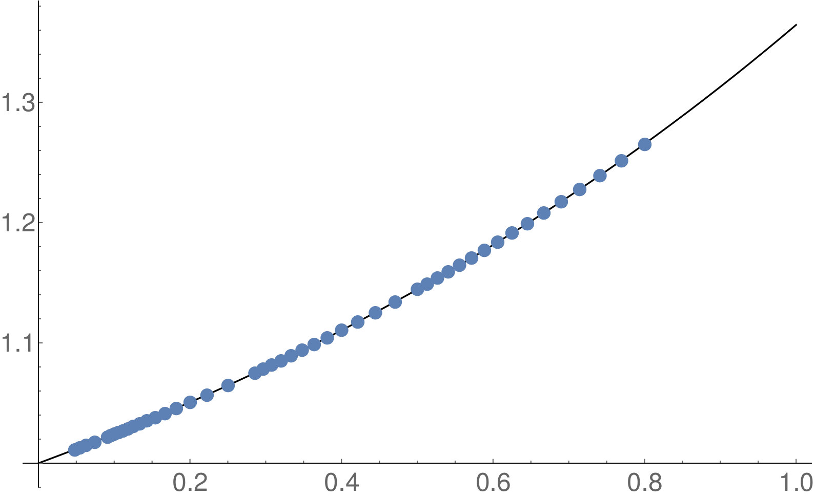 Figure 1
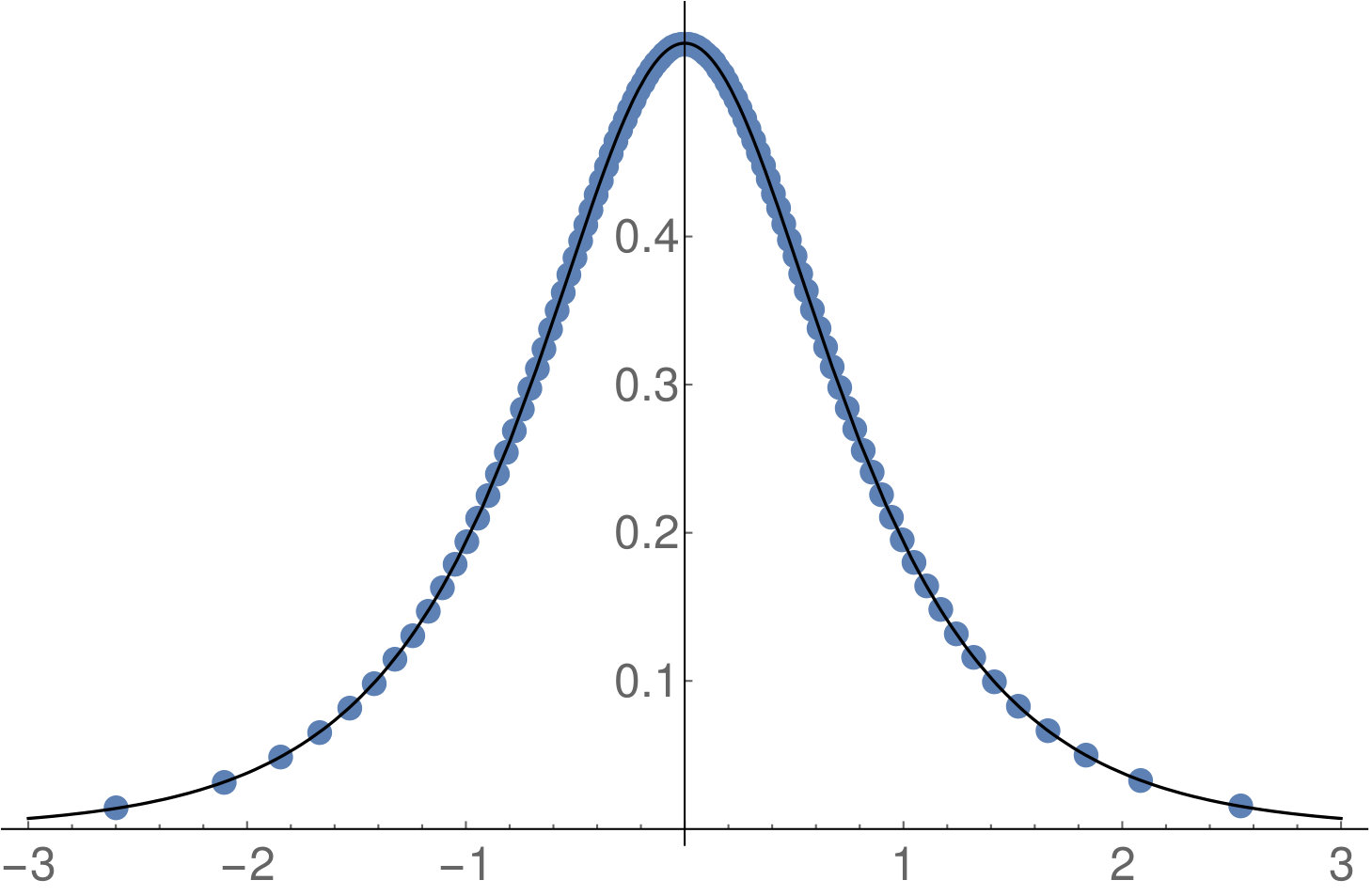 Figure 2
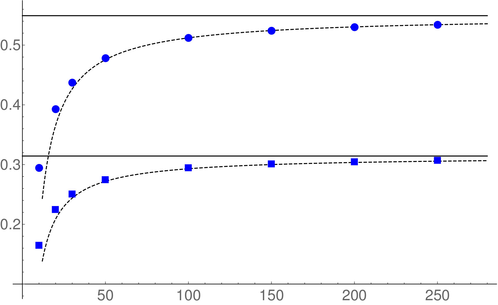 Figure 3
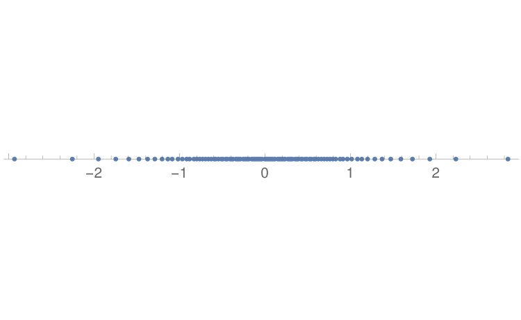 Figure 4
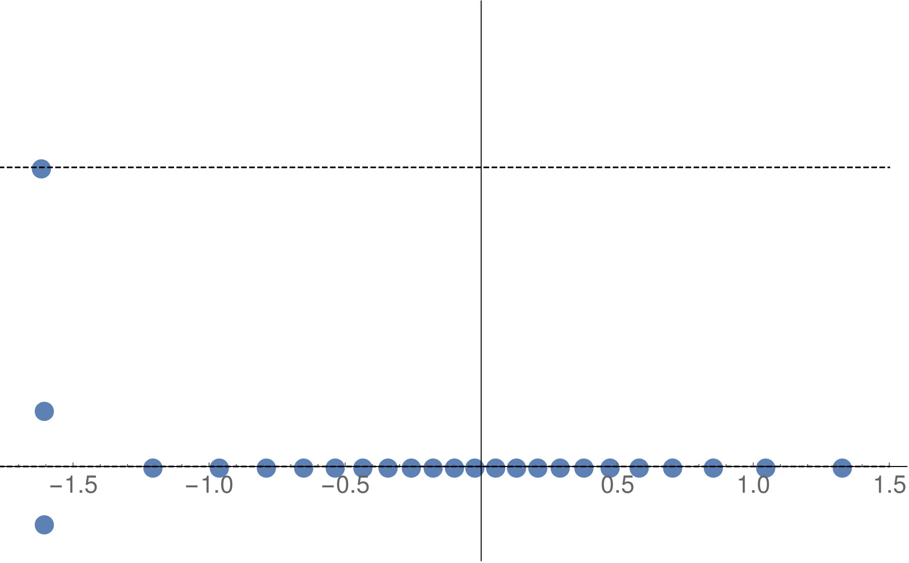 Figure 5
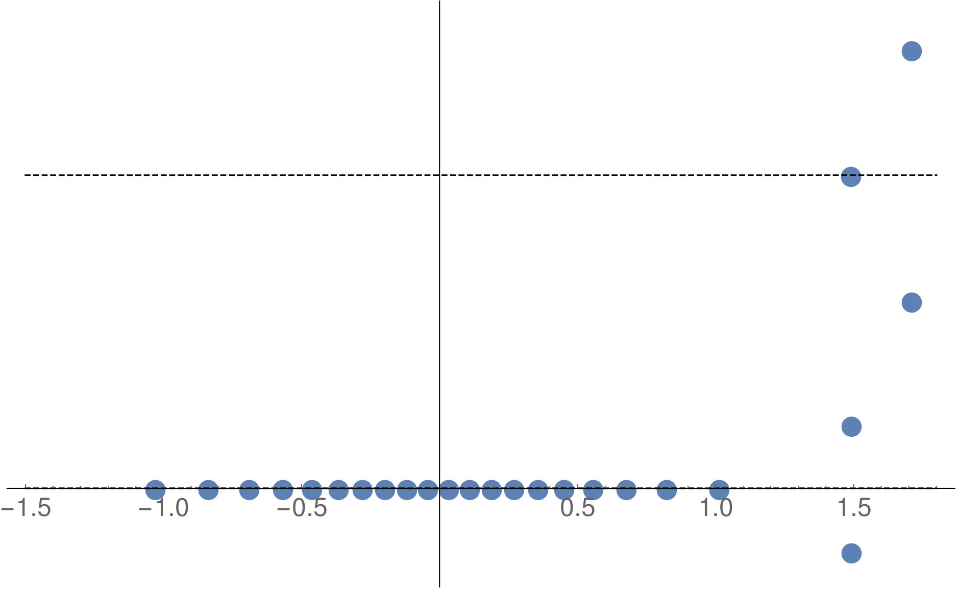 Figure 6
| Parameters | |||||
| Parameters | State | |||||
| “” | ||||||
| “” | ||||||
| “” | ||||||
| “” |
Peer Reviews
No public reviews on file for this paper yet. If you reviewed it on a platform where reviews are public (OpenReview, ICLR, NeurIPS, ICML), you can paste yours below so the community can read it here.
Videos
No videos yet. Explain this paper in a talk, walkthrough, or lecture? Add one.
**Bethe state norms for the Heisenberg spin chain in the scaling limit **
Gleb A. Kotousov1,2 and Sergei L. Lukyanov1,3
1NHETC, Department of Physics and Astronomy
Rutgers University
Piscataway, NJ 08855-0849, USA
2Department of Theoretical Physics
Research School of Physics and Engineering
Australian National University, Canberra, ACT 2601, Australia
and
3Kharkevich Institute for Information Transmission Problems,
Moscow, 127994, Russia
Abstract
In this paper we discuss the norms of the Bethe states for the spin Heisenberg chain in the critical regime. Our analysis is based on the ODE/IQFT correspondence. Together with numerical work, this has lead us to formulate a set of conjectures concerning the scaling behavior of the norms. Also, we clarify the rle of the different Hermitian structures associated with the integrable structure studied in the series of works of Bazhanov, Lukyanov and Zamolodchikov in the mid nineties.
1 Introduction
Consider the Hamiltonian of the Heisenberg spin chain
[TABLE]
subject to the twisted boundary conditions involving the parameter :
[TABLE]
Since it commutes with the -component of the total spin operator they can be simultaneously diagonalized. If we let the “down” spins be at sites , then the (unnormalized) Bethe Ansatz (BA) wave function has the form
[TABLE]
Here stands for the sum over the permutations of and is given by the product of “two-body” factors:
[TABLE]
The quasi-periodicity condition
[TABLE]
leads to a set of equations specifying the admissible values of known as the BA equations:
[TABLE]
with
[TABLE]
The subject of our interest is the normalization sum
[TABLE]
In ref.[1] strong arguments were presented to justify the formulae
[TABLE]
where the elements of the matrix are expressed in terms of (1.6)
[TABLE]
The formula (1.8) was inspired by the original Gaudin hypothesis [2] for the Lieb-Liniger model. Its rigorous proof was given by Korepin in ref.[3].
The Bethe wave function contains an ambiguity related to the choice of the two-body factor . Indeed, the substitution
[TABLE]
where is an arbitrary function of , does not affect the BA equations (1.5). However this changes the overall normalization of the wave function (1.3) (1.4) and, in turn, affects the norm . In what follows we will assume a certain choice for . To describe it explicitly let us parameterize the anisotropy as
[TABLE]
and substitute by the set :
[TABLE]
With this parametrization
[TABLE]
so that the two-body factors in (1.4) can be chosen as
[TABLE]
In the last thirty years impressive progress has been made for the exact calculation of a variety of interesting quantities in the Heisenberg model. However, to the best of our knowledge, we are still lacking a simple analytical tool to study the large- behavior of the norms (1.8)-(1.11). We consider the case with , when the spin chain is critical. Then our numerical analysis suggests that the norms corresponding to the low energy excitations possess the following large- behavior
[TABLE]
It is not difficult to find the exact expressions for the coefficients that define the leading large- asymptotic. Moreover, as the numerical calculation of for the chain with sites requires a negligible amount of computer time nowadays, it is possible to easily determine the scaling exponent and amplitude with a relative accuracy of as long as the anisotropy parameter is not too close to . With the numerical data at hand, one can try to guess the analytical expression for and in (1.12). The main purpose of this work is to formulate a set of conjectures concerning the form of these scaling quantities.
2 RG flow of the low energy Bethe states
Some immediate clarifications are needed for eq. (1.12). In assigning an dependence to the norms, we have in mind a family of Bethe states |\Psi_{L}\big{\rangle} defined for different lengths of the spin chain. For a general lattice system, there are difficulties in introducing the -dependence (RG flow) for individual stationary states. Of course, since the Hilbert space is not isomorphic for different lattice sizes, the problem only makes sense for the low energy part of the spectrum. It is clear how to assign such a dependence for the ground state or, for that matter, the lowest energy states in the disjoint sectors of the Hilbert space. However forming individual RG flow trajectories for low energy stationary states that are densely distributed does not seem to be a trivial task.
In the case under consideration the problem is greatly facilitated by the existence of the BA equations, which are useful to re-write in the logarithmic form
[TABLE]
Here are the so-called Bethe numbers which are integers or half-integers for odd or even respectively. An unambiguous definition of requires fixing the branches of the logarithms in the formulae (1.9), (1.10). Although this is an important step in any practical calculation, we will not touch on it here and only mention that
[TABLE]
for the vacuum state in the sector with fixed value of . For sufficiently large the Bethe numbers corresponding to the low energy states are given by , where the variation from the “vacuum” distribution (2.2) are nonzero only in the vicinity of the edges, i.e., for or . The set can be used to define the individual RG flow trajectories with the following procedure.
Starting with a spin chain for relatively small one can perform the numerical diagonalization of the Hamiltonian. The latter is part of a family of commuting operators, of which a prominent rle is played by the so-called -operator:
[TABLE]
Together with the energies, one should compute the corresponding eigenvalues of which are polynomials,
[TABLE]
whose zeros are related to through eq.(1.9). This allows one to extract the Bethe roots for a certain Bethe state and, using (2.1), also the set . For the state , the BA equations are specified to have the same . Moreover, for their iterative solution the initial approximation can be constructed using the Bethe roots for . This procedure provides a way for defining the RG flow of an individual Bethe state. Finally, the norm entering in the l.h.s. of eq. (1.12) is understood as
[TABLE]
3 Scaling behavior of the Bethe roots
The BA equations (1.5), being written for the set (1.9), form an algebraic system111In this paper it is always assumed that , i.e., .
[TABLE]
In the case of the spin chain in the critical regime, any set solving this algebraic system coincides with its complex conjugate:222This follows from the conjugation condition for the -operator , which implies that all the eigenvalues (2.3) are real analytic functions of .
[TABLE]
This important property allows one to rewrite eq.(1.8), (1.11) in the form
[TABLE]
Let us now give a short sketch of how one can obtain the leading large asymptotic behavior . First consider the vacuum in the sector with given spin . For such a state, if the twist parameter is sufficiently small, all the Bethe roots are real and positive. Using the BA equations one can show that the numbers
[TABLE]
are distributed within the segment with (see fig.1). As most of the roots become densely packed about the origin
so that
[TABLE]
becomes the continuous density and (see fig.2)
[TABLE]
Here we use the parameter
[TABLE]
With these well known facts (see e.g.[4]) it is easy to show that the leading asymptotic behavior of the logarithm of the double product in the r.h.s. of (3.3) grows as with
[TABLE]
At the same time one can argue that in (3.3) goes as , i.e, does not contribute to the leading large asymptotic of the norm. Finally one notes that for the low energy excitations with , the pattern of the Bethe roots are changed essentially only in the vicinity of the edges and the density of the majority of the roots is still given by (3.5). As a result, the leading large- asymptotic of their norms remains the same.
It is a more difficult task to justify the full asymptotic formula (1.12). Nevertheless, numerical work supports this relation. It also shows that the constant remains the same for the low energy states and reads explicitly as
[TABLE]
At the same time both the exponent and the amplitude do depend on the state , i.e, their value is influenced by the roots near the edges of the locus of the Bethe roots distribution.
In the case of the vacuum states, where the Bethe numbers are given by (2.2), all the roots are real and ordered as . For the excited states the roots may become complex and can be ordered w.r.t. their real part
[TABLE]
(the ordering prescription for the Bethe roots with coinciding real parts is not essential for us at this point). When both and go to infinity with kept fixed, the roots and . More accurately for given there exists the following limits
[TABLE]
In these formulae we have used instead of due to the following reason. For one can approximate the Bethe roots by and . It is easy to check that these formulae are consistent with the relations (3.4),(3.5), provided that
[TABLE]
This simple form of the asymptotics justifies the appearance of entering into the definition of the scaling limit (3.8) of the Bethe roots.
4 BA equations in the scaling limit
Keeping in mind the scaling behavior (3.8), one can consider the scaling limit of the BA equations (3.1). To simplify the discussion, we make the technical assumption that . In this case, as it follows from (3.8), with fixed decays faster than so that the l.h.s. of (3.1) turns to be one as . Hence, the BA equations take the form
[TABLE]
where
[TABLE]
Similarly, we can consider (3.1) assuming that is kept fixed as . This leads to equations for the set , which differ from (4.1) only in nomenclature:
[TABLE]
with
[TABLE]
Finally eqs.(4.1) and (4.3) can be rewritten in logarithmic form
[TABLE]
Here we use the notations
[TABLE]
where the convergence of the products are guaranteed by the conditions (3.9) provided that . The low energy Bethe states are distinguished by a specific phase agreement in (4.5), determined by a choice of integers and which play the rle similar to that of the Bethe numbers in (2.1). These integers of course depend on the choice of branches of the logarithm in (4.5). However, once these branches are suitably fixed, every low energy state is characterized by the two sets and .
The parameters and which show up in (4.5) call for some explanation. Since the Hamiltonian of the spin chain (1.1), (1.2) is a periodic function of the twist parameter , relations (4.2) and (4.4) imply that
[TABLE]
where . Below we will refer to the integer as a winding number. It enumerates the different bands of the spectrum of the model. The lowest energy states in the sector with given are of special interest. We will call these the primary Bethe states. The patterns of the Bethe roots are depicted for two such states corresponding to the winding numbers and in fig. 3.
Finally let us note that the functions and (4.6) can be interpreted as a properly defined scaling limit of the eigenvalues of the -operator. Indeed, as it follows from eqs.(2.3), (3.8)
[TABLE]
Notice that in writing eq.(2.3) the -operator was normalized by the condition
[TABLE]
In this case
[TABLE]
5 ODE/IQFT correspondence
It is well known that the scaling behavior of the Heisenberg spin chain is governed by the massless Gaussian model with the Lagrangian density
[TABLE]
Below we use the complex Euclidean coordinates , and denote , . We’ll take and due to the scale invariance, one can set without any loss of generality. The equations of motion imply that and are holomorphic and antiholomorphic fields, respectively, admitting the Fourier series expansions
[TABLE]
The expansion coefficients obey the Heisenberg commutation relations,
[TABLE]
The low energy states of the spin chain in the sector with given form the linear space
[TABLE]
in the scaling limit. Here and stand for the Fock spaces. The Fock space is the highest weight representation with the highest vector , defined by the conditions
[TABLE]
Similarly, the Fock space is the space of the representation of another copy of the Heisenberg algebra generated by .
On the other hand, our analysis in the previous section suggests that the low energy states are characterized by the value of , the winding number and two sets of integers and . As it follows from eq.(2.2), for the vacuum state with , the integers and are consecutive positive numbers
[TABLE]
For a general low energy state the , differ from their “vacuum” values, but stabilize to these for sufficiently large :
[TABLE]
In this section we will briefly explain the link between the two descriptions. Our discussion is based on the ODE/IQFT (Ordinary Differential Equations/Integrable Quantum Field Theory) correspondence, which was developed in the works [5, 6, 7, 8].
In ref.[8], the Schrdinger equation was studied
[TABLE]
with the so-called Monster potentials of the form
[TABLE]
Here the set of complex numbers satisfy the system of algebraic equations
[TABLE]
With these constraints imposed on the positions of the singularities any solution of the Schrdinger equation is monodromy free everywhere except for and for any value of . In other words the solutions remain single-valued in the vicinity of each singularity specified by . For this reason, these points are referred to as apparent singularities.
Assuming that , one can consider the standard spectral problem for the ODE defined on the ray . This leads to a discrete spectral set . It was explained in Appendix A of ref.[8] that this set can be obtained through the solution of the exact Bohr-Sommerfeld quantization condition, which takes the form
[TABLE]
Here , while denotes the spectral determinant that for is given by the convergent product
[TABLE]
For a given Monster potential the integers appearing in the r.h.s. of (5.6) are fixed unambiguously once the branch of the logarithm is specified. Comparison with the scaling form of the BA equation (4.5) suggests that for any low energy state the set of scaling Bethe roots coincides with the spectral set for a certain Monster potential up to an overall factor, provided that the following identifications of the parameters are made
[TABLE]
Using the WKB approximation one can show that for
[TABLE]
where the constant reads explicitly as
[TABLE]
Comparing (5.8) with the asymptotic formula for (3.9) implies that
[TABLE]
The same is of course true for the set , which will correspond to another Monster potential
[TABLE]
characterized by the same value of , but with such that
[TABLE]
and another set .
In ref.[8] it was argued that for given and generic values of , the number of distinct Monster potentials coincides with the number of integer partitions of , i.e., :
[TABLE]
This important property was recently proven by D. Masoero[9]. We now note that the level subspace , which is spanned on the vectors of the form
[TABLE]
has dimensions , i.e., it coincides with the number of distinct Monster potentials for fixed . This suggests that the scaling limit of any low energy Bethe state is described by
[TABLE]
where stands for the norm (2.4). The states , labeled by the set , form the basis in the level subspace . Similarly , labeled by the fully independent set , are a basis of . Thus we can see the emergence of the general structure (5.4) through the scaling limit of the Bethe states. Also (5.4) implies that
[TABLE]
Of course there are many ways to introduce a basis in the level subspaces . The special property of the states is that they are consistent with a certain integrable structure that was studied in refs.[10, 11, 12]. Here we’ll present a few results from those papers. Using the chiral Bose field (5.2) one can construct a commuting set of local Integrals of Motion (IM) with spin :
[TABLE]
By local we mean that each is given by an integral over the local density built out of and its derivatives
[TABLE]
For example, the first three local densities read explicitly as
[TABLE]
The dots in the last line stand for the differential polynomials that involve, together with , also the higher derivatives \partial^{2}\phi,\,\partial^{3}\phi,\ldots\. The set of local IM depend on a single parameter which can be an arbitrary complex number in general. If one makes the identification
[TABLE]
then all the local IM are simultaneously diagonalized in the basis , i.e.,
[TABLE]
The eigenvalues of the first three IM are given by eqs.(29) in ref.[8]. In particular
[TABLE]
The higher spin integrals of motion turn out to be symmetric polynomials of order w.r.t. the variables . In their turn, the level zero eigenvalues are polynomials of order w.r.t. . For example
[TABLE]
Since the local IM act invariantly on each level subspace , the diagonalization problem (5.16) reduces to that of finite dimensional mutually commuting matrices for any given . Let’s present some explicit formulae for for the lowest excited states.
For , when the Monster potential contains only one apparent singularity, the equations (5.5) dramatically simplify. Their solution is
[TABLE]
which is expressed in terms of and , related to and as in eqs. (5), (5.15). Since one has that
[TABLE]
Here is the overall normalization constant, which remains undetermined.
For there are two solutions of eq.(5.5), which will be denoted by and . Explicitly one can show that
[TABLE]
where
[TABLE]
with
[TABLE]
The corresponding basis states are given by
[TABLE]
6 Scaling limit of the norms
The states that appear in the scaling limit (5.11) diagonalize the full set of local IM (5.16). It is expected that for generic values of , this allows one to specify the states up to an overall normalization. To resolve this last ambiguity, we should discuss the natural Hermitian structure appearing in the spin chain and its scaling limit.
The space of states of the spin chain of length is the tensor product of copies of the two-dimensional complex vector space. The positive definite inner product for this space is induced by that of each two-dimensional component. The latter is defined as , where stands for the two basis vectors such that . For generic values of the twist parameter , any two Bethe states corresponding to different solutions of the BA equations turn out to be orthogonal w.r.t. this inner product. We’ll return to this important property later, in sec. 10.
On the other hand, the space admits a natural positive definite inner product specified unambiguously by the conjugation condition for the Heisenberg generators,
[TABLE]
together with the relations for the highest vector
[TABLE]
It is important that this Hermitian structure is consistent with the integrable structure described in the previous section. In particular, all the local IM are Hermitian operators w.r.t. the conjugation (6.1),
[TABLE]
and therefore, for generic values of , one may expect that the states and corresponding to different sets and to be orthogonal. Thus, we come to the conclusion that the natural Hermitian structure in the spin chain of finite length becomes that defined by formulae (6.1) and (6.2) in the scaling limit. Then eq.(5.11) implies that the states form an orthonormal basis in :
[TABLE]
and similarly for . The last condition fixes the overall normalization of up to an inessential sign factor.333 The transformation acts on the Bethe wave function as . As it follows from the formulae (1.3), (1.4), (1.9), (1.11) and (3.2) under the transformation the Bethe state gains an overall phase factor with . By a simple modification of the Bethe wave function, the Bethe state can be adjusted so that . Together with eq. (5.11), this implies that and . Since the transformation acts in the Fock space as , where is a c-number, this allows one to resolve the phase ambiguity in the normalization of and . For example, the undetermined constants in eqs.(5.18) and (5.19) read as follows:
[TABLE]
Let us now turns to the norms appearing in eq. (5.11). Our numerical work led us to the following
Conjecture I: The scaling exponent in the asymptotic formula (1.12) is given by
[TABLE]
while the amplitude factorizes as
[TABLE]
7 Characterizing the Bethe states when is finite
The scaling amplitudes are functions of the set , which label the states in the Fock space. Thus, for their numerical computation using eqs.(1.12),(3.6),(3.7),(6.6),(6.7), we run into an important practical problem: having at hand the Bethe roots corresponding to the Bethe state for a few values of , how to identify its scaling limit, i.e., to extract the sets and characterizing the r.h.s. of eq. (5.11).
The most straightforward approach to the problem is to study the energy corresponding to . In terms of the Bethe roots, it is given by the following expression
[TABLE]
For the critical spin chain, the large- behavior obeys the asymptotic
[TABLE]
Here is the specific bulk energy, which in the case at hand is given by
[TABLE]
while is the Fermi velocity (to be compared with eq. (3.7)):
[TABLE]
In view of eq.(5), the formula (7.1) allows one to extract the integer from the numerical data at finite . However, it is of course insufficient to determine the sets and characterizing the scaling limit of . More information can be obtained from the study of the finite size corrections to the energy, denoted by in eq. (7.1). The leading behavior of was found in ref.[13] (see also [14]). For , it is expressed in terms of the local integrals of motion
[TABLE]
where the constants are known explicitly and are presented in that work. For the case when , the corrections take the form
[TABLE]
Here and are the eigenvalues of the so-called dual non-local integrals of motion and respectively [11]. Contrary to the local IM, it is rather tedious to compute the eigenvalues of these operators for the excited states.
The formulae (7.2), (7.3) are sometimes useful for finding and , especially when , for which the leading behavior of is expressed in terms of the local IM. However, there exists a more effective method for identifying the scaling limit of the Bethe state. To explain it, we first make the following remark. As was mentioned before, the functions and defined in eq. (4.6) can be regarded as the scaling limit of the eigenvalues of the lattice -operator (4.8). It turns out that it is possible to construct the operator acting in the Fock space whose eigenvalue on the state coincides with . For the explicit formulae, we refer the reader to the original papers [11, 12]. Here we just mention that the sets of mutually commuting local and dual non-local IM are generated through the large- operator-valued asymptotic expansion of . For and with , the expansion reads as follows [11, 8]
[TABLE]
Here the constant is given by eq.(5.9), while the numerical coefficients and are not essential for our purposes and can be found in sec. 4 of ref.[8]. The subject of our interest is the operator , which will be referred to as the reflection operator. It commutes with all the IM and can be diagonalized simultaneously with them:
[TABLE]
It is possible to show that the eigenvalue of this operator is related to the Bethe roots for the Bethe state as
[TABLE]
Thus, the eigenvalues and can be extracted numerically from the Bethe roots for sufficiently large (see fig. 4). On the other hand, as will be discussed in the next section, there exists a straightforward procedure to calculate the spectrum of the reflection operator in the Fock space . We found that this was the most effective way of identifying the scaling limit of the Bethe state .
For the eigenvalues of read as follows. For the highest state in the Fock space, is given by [11, 6]
[TABLE]
For the first level state (5.18), the eigenvalue is
[TABLE]
One has that for the two states at the second level, defined by eq. (5.19), the corresponding eigenvalues are
[TABLE]
where .
8 The reflection operator
The reflection operator is closely related to the reflection -matrix of the Liouville CFT. The latter was discussed in detail in the seminal work of the Zamolodchikov brothers [15]. Here, following this paper, we’ll briefly describe its construction.
Consider the Liouville CFT associated with the Lagrangian
[TABLE]
where the space-time is the 2D Euclidean cylinder equipped with the complex coordinates and . Because of the scale invariance, we can assume that . Contrary to the Gaussian model (5.1) the field is not holomorphic for the Liouville CFT. However the component of the energy-momentum tensor,
[TABLE]
satisfies the Cauchy-Riemann equation . Being the periodic field at a given Euclidean time slice, can be expanded in the Fourier series
[TABLE]
The expansion coefficients satisfy the Virasoro algebra commutation relations
[TABLE]
with the central charge
[TABLE]
Similar relations hold true for the antiholomorphic component of the energy momentum tensor. The space of states of the Liouville CFT is classified using the highest weight representations of . The chiral part of this Hilbert space is built from the Verma module containing the primary state :
[TABLE]
Let us introduce the “zero-mode” of the Liouville field
[TABLE]
and consider the asymptotic domain in the configuration space where . Then the exponential interaction in (8.1) is negligible, so that becomes a free massless field that can be expanded in terms of the free field oscillators as in (5.2),(5.3)
[TABLE]
Here is the momentum conjugate to the zero-mode. In the asymptotic domain, the Virasoro generators are represented as follows
[TABLE]
The above relations suggest that the Fock space for can be interpreted as the space of “in”-asymptotic states of the Liouville CFT, while with are identified with the “out”-states (see ref.[15] for a further discussion). In such a situation it is natural to introduce the reflection -matrix intertwining the spaces of in- and out- asymptotic states:
[TABLE]
It is readily established that
[TABLE]
where is a certain phase factor while and are properly normalized operators acting in the chiral Fock spaces. In particular
[TABLE]
The action of the operator is fully determined by the conformal symmetry and is constructed in the following way. One can consider the oscillator basis in the Fock space formed by the vectors
[TABLE]
where stands for the multi-index with . On the other hand, formulae (8) define the structure of the Virasoro highest weight representation on the Fock space with . There is a natural basis in that is associated with this structure
[TABLE]
where again . The two bases are of course linearly related, so that
[TABLE]
The matrix elements of the operator are given by
[TABLE]
It should be emphasized that, since this operator intertwines different Fock spaces, the problem of its diagonalization does not make sense. However one can introduce another intertwiner, the “-conjugation”, whose action is defined by the condition
[TABLE]
so that acts invariantly in the Fock space
[TABLE]
In ref.[15] it was pointed out that this operator commutes with the action of the local IM defined by eqs.(5), (5) with the parameter substituted by . In connection to this, we note that the local IM can be re-written in terms of the field (8.3) and its derivatives only:
[TABLE]
where is the central charge (8.5) of the Virasoro algebra (8.4). In general, one has
[TABLE]
where the dots stand for the terms involving . The limit can be understood as a certain classical limit such that becomes the set of IM for the classical KdV equation [16, 17, 10]. Thus, the operator (8.9) is part of the quantum KdV integrable structure studied in refs.[10, 11, 12]. It should be pointed out that the Liouville reflection -matrix itself is defined by the conformal symmetry alone and does not assume the presence of any integrable structure.
The reflection operator appearing in the previous section is given by
[TABLE]
where the parameters are identified as follows
[TABLE]
Since all the matrix elements {\big{[}s(p)\big{]}^{J}}_{I} are rational functions of , the operator commutes with the local IM in the domain where . A useful relation, that follows immediately from eqs. (8.7),(8.8),(8.12) and (7.8), is that
[TABLE]
for any set .
Formula (8.12) provides an effective tool for the calculation of the spectrum of the reflection operator. The eigenvalues for the first few levels are given by eqs. (7.8)-(7.10). For the higher levels , the eigenvalues of turn out to be rather cumbersome. However their product for a given level , i.e., , admits a remarkably simple structure
[TABLE]
where is the number of integer partitions of .
Significant simplifications occur in the case when . Using the explicit formula (7.9), (7.10) one has
[TABLE]
with . In general, for an arbitrary set , it is possible to show that
[TABLE]
Here are two sets of integers satisfying the condition and also
[TABLE]
In fact, the sets can be used to classify the states for any . The integers , which appear in the exact Bohr-Sommerfeld quantization condition (5.6), are expressed through these numbers (for details, see Appendix A in ref.[8]).
Finally, it is worth noting that the spectral problem for the reflection operator (7.5) turns out to be the most effective procedure for the explicit construction of the basis states .
9 Inner product for the Verma module
The formulae (8.10),(8.11) combined with the Fourier expansion for (8.3) imply that the local IM can be understood as elements of the universal enveloping algebra of without any reference to the Heisenberg algebra. Therefore the diagonalization of the set can be formulated as a problem in the Verma module rather than in the Fock space . Recall that denotes an eigenvector of the local IM at level normalized by the condition (6.4). We now introduce the notation \big{|}{\bm{w}}^{(N)}\big{\rangle}\!\!\big{\rangle} for the eigenvector
[TABLE]
normalized such that
[TABLE]
Here the dots denote the terms involving the Virasoro algebra generators with . The eigenvectors up to level are given by
[TABLE]
Of course, being written in terms of the Heisenberg creation operators via eq. (8), these states coincide up to an overall factor with the highest Fock state , (5.18) and \big{|}{\bm{w}}^{(2,\pm)}\big{\rangle} (5.19), respectively.
The Virasoro algebra possesses the natural Hermitian conjugation
[TABLE]
for any real values of the central charge . It is important to note that when is pure imaginary , i.e., , this does not coincide with the Hermitian conjugation discussed in sec. 6. The latter in this case, as it follows from eq. (8), does not lead to a simple conjugation condition for .
The formula (9.4) can be equivalently rewritten in terms of the holomorphic field :
[TABLE]
In view of eqs.(8.10),(8.11) this implies that
[TABLE]
Thus, the Hermitian conjugation (9.4) is consistent with the quantum KdV integrable structure.
The Verma module has a unique Hermitian form that is induced from the conjugation (9.4) and such that the norm of the highest vector is one. Because of the Hermiticity of the local IM (9.5), this Hermitian form is diagonal in the basis of the eigenstates \big{|}{\bm{w}}\big{\rangle}\!\!\big{\rangle} (9.1), (9.2):
[TABLE]
For example, for the states (9) at the first few levels one has
[TABLE]
where . Notice that the product of for all the states with given coincides with the Gram determinant for (9.6) restricted to this level. The calculation for the lowest levels leads to
[TABLE]
This is reminiscent of the Kac determinant formula [18]. However, contrary to the latter, the factor does depend on and for . In particular
[TABLE]
In the l.h.s. of eq.(9.6) we use the subscript to emphasize that the inner product is calculated using the natural Hermitian conjugation (9.4) for the Virasoro algebra. On the other hand, one can treat \big{|}{\bm{w}}\big{\rangle}\!\!\big{\rangle} and \big{|}{\bm{w}}^{\prime}\big{\rangle}\!\!\big{\rangle} as states from the Fock space and calculate their inner product using the Hermitian conjugation for the Heisenberg algebra. The result, of course, is different:
[TABLE]
The relations (8.7), (8.12) imply that
[TABLE]
10 Star conjugation for the finite spin chain
We now turn to the main subject of this paper – the norm (1.8), or equivalently (3.3). In fact, instead of it is useful to focus on the combination
[TABLE]
Here
[TABLE]
and relations (7.6), (7.7) imply the following scaling behavior for this quantity
[TABLE]
Combining these with eqs.(1.12),(3.7),(6.6),(6.7) one finds
[TABLE]
with the scaling exponent given by
[TABLE]
The amplitudes and are related to and in (6.7) as
[TABLE]
The motivation for studying comes from Korepin’s approach to the norms in ref.[3], which is based on the Quantum Inverse Scattering Method. In this framework, the main player is the quantum monodromy matrix that is built from the ordered product of the elementary transport matrices:
[TABLE]
In particular, provided the following identifications are made
[TABLE]
and taking into the account that the Hamiltonian in ref.[3] differs from (1.1) by means of the similarity transformation with the matrix444In this formula is assumed to be even.
[TABLE]
the Bethe state corresponding to the wave function (1.3),
[TABLE]
can be nicely expressed in terms of the operators555In the l.h.s. of this relation we use the argument instead of . It is easy to see that the operator is a single valued function of this variable.
[TABLE]
Namely, one has
[TABLE]
Here stands for the pseudo-vacuum
[TABLE]
Notice that the states (10.10) diagonalize the transfer-matrix
[TABLE]
The latter is related to the Hamiltonian (1.1) as
[TABLE]
Using eq. (10.10) and that coincides with the complex conjugated set, the norm can be represented as
[TABLE]
On the other hand, a simple calculation based on the definitions (10.7) and (10.9) shows that
[TABLE]
where the operator is defined similarly to (10.9):
[TABLE]
Thus eq.(10.12) takes the form
[TABLE]
In ref.[1] Gaudin, McCoy and Wu conjectured that the above norm coincides with the r.h.s. of eq. (1.8) with taken as in eq.(1.11). This was proven in the work [3].
Let us rewrite eq.(10.13) in terms of defined by (10.1):
[TABLE]
We now note that (10.2) coincides with the eigenvalue of the operator
[TABLE]
built from the -operator. Then with eq. (10.14) one can interpret to be the norm of the Bethe state \prod_{m=1}^{M}{\hat{\bm{\mathsf{B}}}}(\zeta_{m})\,\big{|}\,0\,\big{\rangle} w.r.t. the “star” conjugation, which is related to the ordinary matrix conjugation {\hat{\mathsf{O}}}^{\dagger}\equiv\big{(}{\hat{\mathsf{O}}}^{T}\big{)}^{*} as
[TABLE]
In view of eqs.(9.6), (9.8), (9.9), (10.1), (10.3) the star conjugation (10.16) for the spin chain with finite length becomes and for in the scaling limit.
For any operator commuting with , one has that . In particular, it is easy to show that for the transfer-matrix (10.11)
[TABLE]
When the twist parameter , the transfer-matrix is expected to lift all the degeneracies in the basis of the stationary states, so that \prod_{m=1}^{M}{\hat{\bm{\mathsf{B}}}}(\zeta_{m})\,\big{|}\,0\,\big{\rangle} corresponding to different sets turn out to be orthogonal w.r.t. the inner products associated with both the “dagger” and “star” conjugations. Finally, we note that the norm corresponding to the star conjugation is not positive definite.
11 Outcomes of numerical work
Unfortunately we don’t know of any analytic techniques that could allow one to derive the scaling behavior of the norms of the Bethe states (1.12), including explicit expressions for the scaling exponent and amplitude . However, through numerical work, we conjectured the formula (6.6) for , and found that obeys the factorized structure (6.7). The latter, as a consequence of eq.(10.6) can be written in the form
[TABLE]
Recall that , and . In sec. 8, we discussed how to compute the eigenvalues () of the reflection operators entering into the above formula. Thus, we are left to describe the unknown factors and . Since there is only a nomenclature difference between the two, it is sufficient to focus on only.
In order to present the results of our numerical study, we will first define some special functions and briefly describe their properties.
11.1 The special functions
Introduce the notation
[TABLE]
Notice that the scaling exponent (10.5) is given by
[TABLE]
Then, the function is defined through the convergent product
[TABLE]
Here and are the Glaisher and Euler constants, respectively, while plays the rle of the parameter which is always assumed to be positive. It follows from the definition that is an entire function of whose zeros are located on the real negative semi-axis at the points
[TABLE]
As the function possesses the asymptotic behavior
[TABLE]
In many situations it is convenient to use the integral representation
[TABLE]
which is valid in the half plane . Note that this formula immediately implies that satisfies the “duality” relation
[TABLE]
Similar to (11.4), we define another function :
[TABLE]
that obeys the relation
[TABLE]
Contrary to (11.4) it is possible to explicitly evaluate the integral in eq.(11.5), which yields
[TABLE]
Notice that, using the function , eq.(7.8) can be rewritten as
[TABLE]
Finally we define the entire function
[TABLE]
which for admits the integral representation
[TABLE]
For any complex the value of can be found by means of the convergent product
[TABLE]
11.2 Conjectures
Through a numerical study of the norms in the scaling limit, we were lead to the following
Conjecture II: In the case of the primary Bethe states, which correspond to the level ,
[TABLE]
Here the constants are independent of and depend only on the parameter .
Fig. 5 depicts as a function of . Notice that for the spin chain can be reformulated as a non-interacting system of 1D lattice fermions. In this case, and one can show that
[TABLE]
We found it useful to re-write the other constant appearing in eq. (11.8) in the form
[TABLE]
Then for the free fermion case
[TABLE]
Moreover, within the accuracy of our calculations, in the domain .
Conjecture III: For a general Bethe state
[TABLE]
where is defined by eqs. (9.6), (9.1), (9.2) and the constants are the same as in eq. (11.8). This formula was numerically verified for (for an illustration, see tabs. 1 and 2).
Eq.(11.10) supplemented by (11.1), (9.9), (11.6), (11.7) implies the following result for the scaling amplitude from (1.12):
[TABLE]
The state dependent factor is unambiguously defined by eqs. (9.1), (9.2), (9.8). For the primary Bethe states one has that .
The following comment is in order here. In the case when , i.e., , an explicit analytical expression for the norm at finite was conjectured for certain primary Bethe states by Razumov and Stroganov in refs.[19, 20]. In our conventions, the expressions proposed in those works translate to
[TABLE]
where
[TABLE]
is the number of alternating sign matrices. It is straightforward to show that the large- behavior of (11.2) is consistent with our results (1.12), (6.6), (11.11), provided that
[TABLE]
12 Conclusion
This work is dedicated to the description of the scaling behavior of the norms of the low energy states of the spin chain in the critical regime, where the anisotropy . The key result is the formula (1.12) supplemented by the explicit expressions for the constants (3.6), (3.7), the state dependent exponent (6.6) and the scaling amplitude (11.11). The result was obtained by a combination of analytical techniques based on the ODE/IQFT correspondence and the numerical analysis of the norms. Currently, all the above mentioned formulae have a conjectural status. We believe that their rigorous proof would give a better understanding of the scaling limit of integrable lattice models and, perhaps, general aspects of the RG flow for systems in dimensions.
Another result which deserves to be mentioned is the Hermitian conjugation for the finite chain given by eqs. (10.16) and (10.15), which induces the canonical conjugation (9.4) of the conformal algebra in the scaling limit. Clearly, such a modification of the conventional matrix Hermitian structure can be interpreted as the lattice counterpart of the Dotsenko-Fateev procedure of introducing the “charge at infinity” in the Gaussian model [21]. This is of prime importance for the RSOS restrictions of the 6-vertex model [22]. One can note that, typically, in lattice integrable systems the Bethe states are not orthogonal w.r.t. the naive inner product as the standard matrix conjugation does not have any meaningful intrinsic description in the algebra of commuting - and - operators. An interesting example of such a phenomenon is provided by the alternating spin chain associated with the inhomogeneous 6-vertex model [23]. In this case the Hermitian conjugation, which is consistent with the integrable structure of the model, becomes the canonical one for the -algebra underlying the scaling behavior of the lattice system. A detailed study of the interplay of these Hermitian and integrable structures is of prime importance for understanding the scaling limit of the alternating spin chain [24]. Some results in this direction were reported in the recent work [25].
Acknowledgments
The authors thank V. Bazhanov, G. Korchemsky, I. Kostov, V. Mangazeev, H. Saleur, F. Smirnov and A. Zamolodchikov for stimulating discussions and important comments.
The final stage of this work was done during the second author’s visit to the IPhT Centre CEA de Saclay. SL is grateful to the IPhT for its support and hospitality.
The reference list from the paper itself. Each links out to its DOI / PubMed record.
- 1[1] M. Gaudin, B. M. Mc Coy and T. T. Wu, “ Normalization sum for the Bethe’s hypothesis wave functions of the Heisenberg-Ising chain ”, Phys. Rev. D 23 , 417 (1981) [https://journals.aps.org/prd/abstract/10.1103/Phys Rev D.23.417] .
- 2[2] M. Gaudin, Saclay Report Nos. CEA-N-1559(1), 1972 (unpublished); Saclay Report Nos. CEA-N-1559(2), 1972 (unpublished); “ The Bethe Wavefunction ”, Cambridge: Cambridge University Press (2014) [https://doi.org/10.1017/CBO 9781107053885] . · doi ↗
- 3[3] V. E. Korepin, “ Calculation of norms of Bethe wave functions ”, Commun. Math. Phys. 86, 391 (1982) [https://projecteuclid.org/euclid.cmp/1103921777] .
- 4[4] R. J. Baxter, “ Exactly solved models in statistical mechanics ”, London: Academic Press (1982) [https://physics.anu.edu.au/theophys/ files/Exactly.pdf] .
- 5[5] P. Dorey and R. Tateo, “ Anharmonic oscillators, the thermodynamic Bethe ansatz, and nonlinear integral equations ”, J. Phys. A 32 , L 419 (1999) [ar Xiv:hep-th/9812211] .
- 6[6] V. V. Bazhanov, S. L. Lukyanov and A. B. Zamolodchikov, “ Spectral determinants for Schroedinger equation and Q-operators of conformal field theory ”, J. Stat. Phys. 102 , 567 (2001) [ar Xiv:hep-th/9812247] .
- 7[7] J. Suzuki, “ Functional relations in Stokes multipliers – Fun with x 6 + α x 2 superscript 𝑥 6 𝛼 superscript 𝑥 2 x^{6}+\alpha x^{2} potential ”, J. Stat. Phys. 102 , 1029 (2001) [ar Xiv:quant-ph/0003066] .
- 8[8] V. V. Bazhanov, S. L. Lukyanov and A. B. Zamolodchikov, “ Higher-level eigenvalues of Q-operators and Schroedinger equation ”, Adv. Theor. Math. Phys. 7 , 711 (2003) [ar Xiv:hep-th/0307108] .