A Chance-Constrained Stochastic Electricity Market
Yury Dvorkin

TL;DR
This paper introduces a chance-constrained stochastic market design that effectively manages renewable energy uncertainty, ensuring robust prices and social welfare in electricity markets, demonstrated through a case study on the ISO New England testbed.
Contribution
It proposes a novel chance-constrained stochastic market framework that internalizes renewable uncertainty and guarantees non-confiscatory outcomes in expectation and per scenario.
Findings
Produces a robust competitive equilibrium under uncertainty
Internalizes renewable resource uncertainty in price formation
Validated through a case study on ISO New England testbed
Abstract
Efficiently accommodating uncertain renewable resources in wholesale electricity markets is among the foremost priorities of market regulators in the US, UK and EU nations. However, existing deterministic market designs fail to internalize the uncertainty and their scenario-based stochastic extensions are limited in their ability to simultaneously maximize social welfare and guarantee non-confiscatory market outcomes in expectation and per each scenario. This paper proposes a chance-constrained stochastic market design, which is capable of producing a robust competitive equilibrium and internalizing uncertainty of the renewable resources in the price formation process. The equilibrium and resulting prices are obtained for different uncertainty assumptions, which requires using either linear (restrictive assumptions) or second-order conic (more general assumptions) duality in the price…
Click any figure to enlarge with its caption.
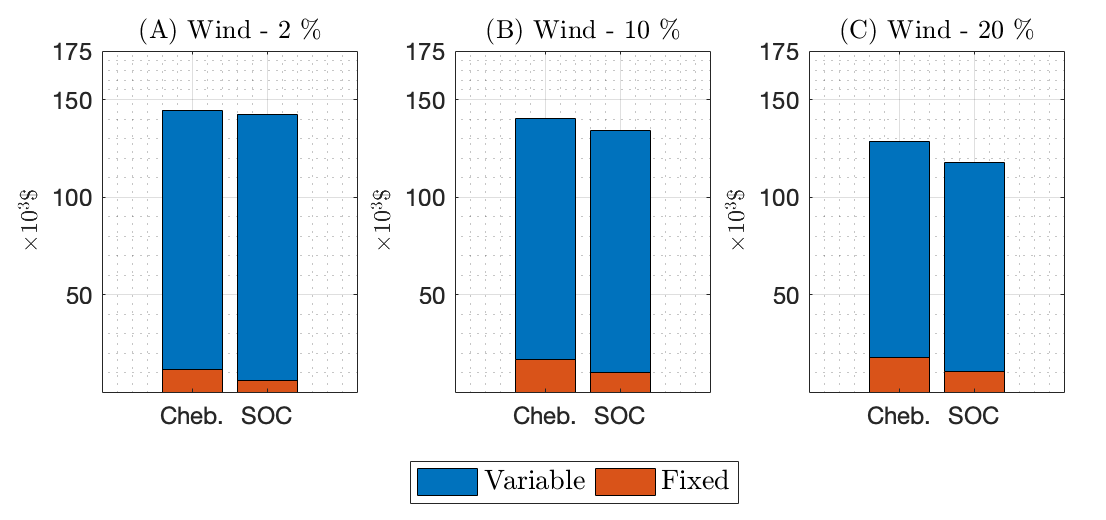 Figure 1
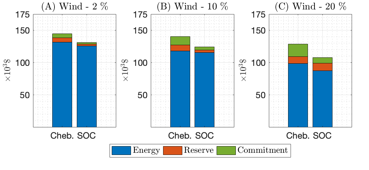 Figure 2
 Figure 3
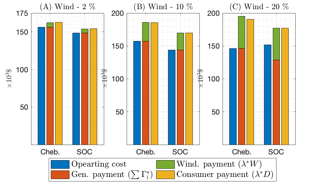 Figure 4
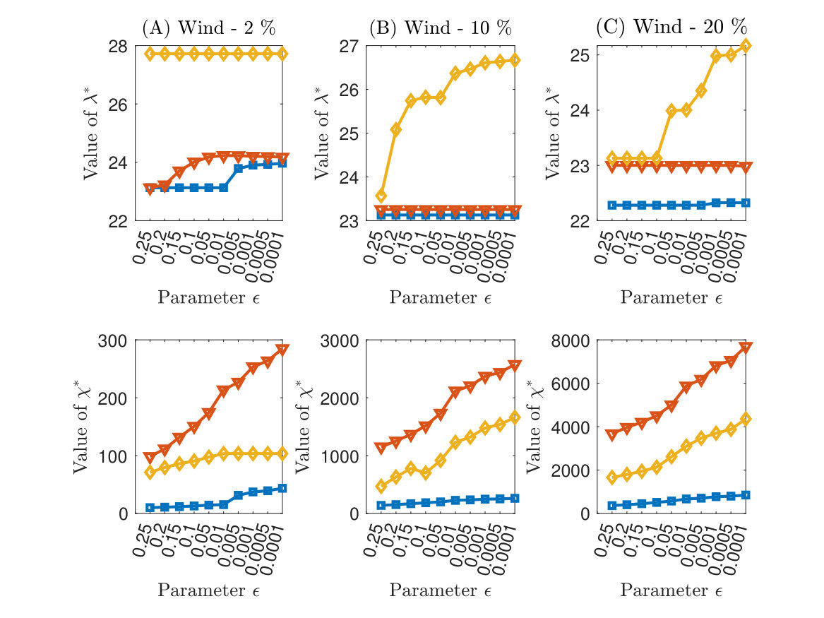 Figure 5
Peer Reviews
No public reviews on file for this paper yet. If you reviewed it on a platform where reviews are public (OpenReview, ICLR, NeurIPS, ICML), you can paste yours below so the community can read it here.
Videos
No videos yet. Explain this paper in a talk, walkthrough, or lecture? Add one.
A Chance-Constrained Stochastic Electricity Market
Yury Dvorkin, IEEE, Member Yury Dvorkin is with the Department of Electrical and Computer Engineering, Tandon School of Engineering, New York University, New York, NY 11201 USA (e-mail: [email protected]). This work was supported by the U.S. National Science Foundation under Grants # ECCS-1760540, CMMI-1825212, ECCS-1847285 and by the Alfred P. Sloan Foundation under Grant # G-2019-12363.
Abstract
Efficiently accommodating uncertain renewable resources in wholesale electricity markets is among the foremost priorities of market regulators in the US, UK and EU nations. However, existing deterministic market designs fail to internalize the uncertainty and their scenario-based stochastic extensions are limited in their ability to simultaneously maximize social welfare and guarantee non-confiscatory market outcomes in expectation and per each scenario. This paper proposes a chance-constrained stochastic market design, which is capable of producing a robust competitive equilibrium and internalizing uncertainty of the renewable resources in the price formation process. The equilibrium and resulting prices are obtained for different uncertainty assumptions, which requires using either linear (restrictive assumptions) or second-order conic (more general assumptions) duality in the price formation process. The usefulness of the proposed stochastic market design is demonstrated via the case study carried out on the 8-zone ISO New England testbed.
I Introduction
Following the restructuring of the power sector in the US and many European nations, wholesale electricity markets have become instrumental for unleashing competitive forces that, at least theoretically, should encourage efficiency improvements among electricity suppliers and eventually reduce the cost of electricity for consumers. For example, PJM reports that their market has annually saved up to $2.3 billion and reduced wholesale electricity prices by 40% in 2008-2017 [1]. However, there is a growing concern that the ability of existing electricity market designs to continue delivering these benefits will drastically diminish, as the current trend to massively deploy large-scale renewable resources continues. This concern is mainly attributed to the uncertainty and limited controllability of renewable resources, as well as their zero or near-zero production costs, which tend to distort market outcomes by dispatching thermal generators in an out-of-merit order [2, 3]. To account for the effect of constantly increasing uncertainty on market outcomes, Morales et al. [4] redefine the merit order to include the expected cost of uncertainty, in addition to the original marginal cost of production, associated with increased reserve needs due to the presence of renewable resources. Therefore, consistent with the motivation in [4, 2, 3], the US Department of Energy emphasizes the need for ‘market structures such as ancillary services, balancing markets and energy markets [that] maintain their competitive frameworks […] as resource mixes change to assure that the market rules are providing the appropriate signals to bring forth both long-term and short-term electricity supplies’ [5].
This need has paved the way for new market mechanisms, commonly referred to as stochastic market designs, that are capable of holistically modeling probabilistic characteristics of renewable resources, e.g., by means of scenario-based stochastic programming. To a large extent, these mechanisms are enabled by the seminal work of Papavasiliou and Oren [6], which demonstrated the economic savings of scenario-based stochastic programming attained from reducing overly conservative deterministic reserve margins [6]. Thus, instead of using conservative, exogenously set margins (e.g., -rule as in [6]), uncertain and variable outputs of renewable resources can be represented via a finite set of scenarios and their corresponding probabilities. This leads to a lower expected and ex-post operating cost and, under the assumption of inflexible demand, maximizes the social welfare. While this welfare-maximization is a desired property of any market design, existing stochastic market designs struggle to achieve it simultaneously with two other desired properties – revenue adequacy, i.e., the payments collected by the market from consumers are greater or equal to the payments made by the market to producers, and cost recovery, i.e., the payment to each producer is greater or equal to its operating cost111Current deterministic US markets also use out-of-market corrections and uplift payments to retain market participants.. Furthermore, in the specific case of scenario-based stochastic programming, achieving revenue adequacy and cost recovery is difficult since it must be done for both the expected case and each scenario individually. For instance, Pritchard et al. [7], Morales et al. [8] and Wong et al. [9] demonstrated that revenue adequacy and cost recovery are satisfied in expectation, but do not necessarily hold for individual scenarios. Kazempour et al. [10] and Ruiz et al. [11] simulated a stochastic electricity market using stochastic equilibrium problems to simultaneously ensure cost recovery and revenue adequacy per scenario and in expectation. However, the market designs in [11, 10] do not guarantee social welfare maximization and, therefore, are intended by the authors for market analyses rather than market-clearing tools. As discussed in [10], a lack of cost recovery and revenue adequacy guarantees inhibits implementing scenario-based stochastic market designs in practice. As a result, rare real-world stochastic electricity markets are limited to exogenous sizing of probabilistic security margins (reserves) within otherwise deterministic market-clearing routines, e.g., in Swissgrid [12].
Realizing the shortcomings of scenario-based stochastic programming described above, this paper offers a different perspective on a stochastic market design. Instead of modeling uncertain outputs of renewable resources by means of a set of scenarios as in [7, 8, 9, 13, 10, 11, 12], one can exploit a chance-constrained approach to internalize the stochasticity of renewable resources in market-clearing tools using statistical moments of the underlying uncertainty (e.g., mean and standard deviation). This approach leads to chance (probabilistic) constraints that, in turn, can be exactly reformulated into convex, deterministic expressions and solved efficiently at scale [14, 15]. Furthermore, these chance constraints offer a high degree of modeling fidelity to control uncertainty assumptions (e.g., probability distributions [16, 17]) and risk tolerance (e.g., the likelihood of constraint violations [16, 15, 14, 18]). Replacing a set of scenarios with its statistical moments using chance constraints not only offers a more accurate representation of uncertainty in market-clearing and dispatch tools, see comparison in [16, 17, 15], but also eliminates the need to trade-off between expected and per scenario performance, while immunizing the resulting market outcomes against uncertainty. That is, a stochastic solution is obtained at the expense of solving a deterministic optimization problem, which internalizes statistical moments and risk parameters in the price formation process.
This paper proposes an alternative stochastic market design that uses chance constraints to accurately model uncertainty of renewable resources. Relative to scenarios, which are often difficult to obtain, the chance constraints can be formulated using statistical moments of uncertain quantities, which are readily available from historical observations222Such historical observations can either be collected by the market operator from their day-to-day operations, or obtained from public repositories supported by the US National Aeronautics and Space Administration and National Oceanic and Atmospheric Administration [17], or licensed/purchased from third-party data providers [19]. [17], and internalize this uncertainty in market-clearing tools. To this end, we formulate a two-stage chance-constrained unit commitment (CCUC) problem that follows pool-market assumptions typical for US wholesale electricity markets. Within this CCUC problem, we consider three different assumptions on underlying uncertainty. First, we assume that the uncertainty is represented by a normal distribution. In this case, the CCUC problem is reduced to a mixed-integer linear program (MILP) that can be used for pricing electricity similarly to the current US practice (e.g., as in [20, 21]). Second, to better accommodate realistic uncertainty, which is often not normally distributed [22], and quadratic production costs of thermal generators, we formulate distributionally robust chance constraints and approximate them using the Chebyshev approximation, leading to a mixed-integer second-order conic (MISOC) program. Third, since the Chebyshev approximation is notoriously conservative, we invoke an exact second-order conic (SOC) reformulation of distributionally robust chance constraints from [23], which also renders a MISOC program. Note that the second and third assumptions cannot be accommodated for electricity pricing by means of linear duality theory, as in [20, 21], and thus the resulting MISOC programs require using more general SOC duality. This paper proves that the MISOC equivalents of the CCUC problem yield a robust competitive equilibrium and analyzes electricity prices obtained by means of SOC duality. In addition to its superior computational performance relative to scenario-based stochastic programming [15], using the CCUC for electricity pricing is advantageous in several aspects. First, the market-clearing procedure does not rely on scenarios and produces a single set of market decisions. Hence, market participants, who are currently distrustful of a scenario-based stochastic market with scenario parameters they do not control [10], will not be exposed to risk of losses. Second, the prices obtained from the proposed market internalize uncertainty and risk parameters in the price formation process, without trading off between expected and per scenario performance. As a result, the proposed chance-constrained market design enables real-world implementations of stochastic electricity markets.
II Stochastic Market via Chance Constraints
Following the current US practice, we formulate a two-stage CCUC problem that optimizes the power production for a single time instance in the future, where the only source of uncertainty stems from wind power generation:
[TABLE]
where is a binary decision on the on/off status of controllable generator from set and is the power output of this generator under uncertainty . Similarly to the current practice, in which the market operator provides forecasts and estimates the reserve requirements, it is assumed that forecasts and , as well as parameters characterizing uncertainty (e.g., distribution and statistical moments), are released by the market operator and are common for all market participants. Assuming that common forecasts are shared among market participants makes it possible to neglect the effects of information asymmetry that can be exploited by strategically acting market participants with proprietary (and different from the market) information, see [24]. Eq. (1a) minimizes the expected operating cost given decisions and and production cost of each controllable generator given by coefficients , and . The output of generator under uncertainty is modeled using a proportional control law in (1b), where is a scheduled power output and is a reserve participation factor. Note that the control law in (1b) assumes that recourse decision is parameterized in terms of first-stage decisions and , which corresponds to preventive security when the operator aims to withstand uncertainty realizations without corrective control actions. Alternatively, one can replace (1b) with a corrective recourse as explained in [25]. The joint, two-sided chance constraint in (1c) ensures that is within the minimum () and maximum () power output limits with the probability given by , where is a small number that represents the tolerance of the market to constraint violations. We assume that wind producers are modeled as undispatchable price-takers with the uncertain power outputs of , where is a given forecast and is its uncertainty. Eq. (1d) ensures that participation factor , if controllable generator is offline, i.e., , and attains a non-negative value from its domain range , if otherwise. The system-wide power balance is enforced in (1e), which balances the total output of conventional and wind power generation resources and demand. Eq. (1f) ensures the sufficiency of reserve provided by controllable generators to cope with uncertainty . The decision variables are declared in (1g). Solving the CCUC in (1) depends on the treatment of (1c) and the assumptions made on as discussed below.
II-1 Approximation by individual chance constraints
To avoid dealing with the joint, two-sided chance constraint in (1c), it is common to invoke two ad-hoc assumptions that follow from power system practices. First, it is assumed that violations on different generators are independent of one another during normal (steady-state) power system operations. Second, simultaneous violations of the minimum and maximum output limits on a given conventional generator are impossible. As a result, (1c) can be approximated by the following separate, one-sided chance constraints:
[TABLE]
[TABLE]
Note that (2c)-(2d) are derived only using and and do not assume a particular parametric distribution (e.g., normal). Thus, using the result in (2c)-(2d) in (1a) and invoking that to reformulate (2a)-(2b), the CCUC problem in (1) is recast as:
[TABLE]
where is a given parameter and is the inverse cumulative distribution function of the standard normal distribution. Note that, if in (3), it follows from (3d) that and due to (3b)-(3c). While the constraints of (3) are linear, the objective function in (3a) is quadratic, thus turning (3) into a mixed-integer quadratic program (MIQP), which can be solved by off-the-shelf solvers (e.g., CPLEX, Gurobi).
II-2 Approximation by the Chebyshev inequality
While the normal assumption on in (3) fares well in practice, e.g., [15, 14], it introduces some inaccuracies as empirically measured uncertainty does not follow this distribution exactly, e.g., [22, 17]. To overcome this limitation, can be modeled using a set of distributions, rather than a single distribution as in (3):
[TABLE]
where uncertainty set encapsulates all probability measures with given first- and second-order moments and . Assuming makes it possible to recast (1c) as distributionally robust chance constraints [27, 23, 28]:
[TABLE]
Applying the Chebyshev inequality to (5) as described in [27, 23, 28], the CCUC problem in (1) can be replaced with:
[TABLE]
where . Similarly to (3), (6) is a MIQP that can be solved efficiently with off-the-shelf solvers. Although adjusting parameter allows for better fitting of empirical data on uncertainty , the accuracy of the Chebyshev approximation reduces when and its solution becomes unnecessarily conservative or may even be infeasible, [23]. Note that in (6) can be chosen such that , i.e., (3) and (6) yield identical solutions.
II-3 Exact SOC reformulation
Motivated by the need to overcome the conservatism of the Chebyshev approximation in (6), Xie and Ahmed [23] derived an SOC equivalent of (1c). Using [23, Theorem 2], the CCUC problem in (1) is equivalent to:
[TABLE]
where and are auxiliary variables and (7b)-(7d) are exact equivalents of (1c). Relative to the optimization in (3) and (6) that only have linear constraints, the notable difference of (7) is constraint (7d), which is a SOC constraint.
II-A Pricing with Chance Constraints via LP duality
II-A1 Prior work
Motivated by the current practice of electricity markets to use LP duality for obtaining electricity prices, [21] proposed to reduce the MIQP in (3) to a linear program (LP) by invoking two restrictive assumptions that , i.e., , and , which leads to the following MILP:
[TABLE]
Remark 1**.**
The MILP in (8) can be related to currently used deterministic market-clearing procedures, if the reserve contribution of each controllable generator is expressed in terms of . Indeed, the upward () and downward () reserve margins in (8b) and (8c) due to can be computed as . Accordingly, the total upward and downward reserve requirement allocated in (8) can be computed as .
While the MILP in (8) cannot be used for pricing electricity directly due to the presence of binary variables , which prevents computing dual variables of binding constraints, it can be converted into an equivalent LP problem, which can be used for electricity pricing as proven in [20, 21]. First, (8) is solved using a MILP solver (e.g., CPLEX, Gurobi) to obtain the optimal values of binary variables . Second, the following LP equivalent of (8) is solved to obtain dual variables:
[TABLE]
where variables are converted into real-valued variables and (9g) sets the value of this variable to . Since (8) and (9) yield the same optimal solution, as proven in [20, 21], dual variables , , and of constraints (9d)-(9g) can be leveraged for electricity pricing. Next, [21] defines the robust competitive equilibrium as follows:
Definition 1**.**
A robust competitive equilibrium for the stochastic market defined by (8) is a set of prices and a set of dispatch decisions that (i) clear the market, i.e., and , and (ii) maximize the profit of individual generators.
We now prove that (8) and (9) return this equilibrium in the following theorem:
Theorem 1**.**
Let be an optimal solution of (8) and let be dual variables of (9). Then constitutes a robust competitive equilibrium, i.e.:
The market clears at and . 2. 2.
Each producer maximizes its profit under the payment of .
Proof.
See our previous work in [21]. ∎
In other words, Theorem 1 establishes that dual variables , , and represent prices for energy, reserve, and commitment allocations that attain the least-cost solution and support a market equilibrium, i.e., no generator has any incentive to deviate from the solution of (8). Similarly to the current electricity markets, Theorem 1 entitles every generator to receive the following three payments: (i) for the energy produced, (ii) for the reserve provided, and (iii) for the commitment status.
II-A2 Extensions of prior work
While still using the LP duality as in [20], we extend the results from [21] by demonstrating that prices , , and internalize both uncertainty () and risk () parameters. Consider the stationary conditions of (9):
[TABLE]
where denotes the Lagrangian function of (9):
[TABLE]
Using the stationary conditions in (10) and , prices , , and can be expressed as follows:
[TABLE]
As per (12), reserve price explicitly depends on , and , while energy and commitment prices and depend on these parameters implicitly via dual variables of inequality constraints and . Unlike the scenario-based stochastic market designs in [7, 9, 8, 10, 13], the prices in (12) incorporate uncertainty and risk parameters without the need to consider multiple scenarios and trading off among per scenario and expected performance. Notably, if inequality constraints in (9b) are not binding, i.e., , these prices reduce to , and that matches the prices of the deterministic market design implemented based on [20].
Remark 2**.**
The results in Theorem 1 and in (12) are obtained for the optimization in (8) under the assumption that and . However, the former assumption can be overcome by adjusting the value of . For example, if the actual uncertainty is modeled as and the desired tolerance to constraint violations is given by , the optimization (8) is still applicable, despite the underlying assumption that , if in (8b)-(8c) is selected such that .
Remark 3**.**
Since Theorem 1 is obtained by reducing (1) to a MILP and proved using the same procedure as in [20], this market design inherits the same cost recovery and revenue adequacy properties as the market design in [20] (which currently underlies US markets), i.e., it requires an uplift payment to each generator equal to to reflect the cost of commitment decisions.
Using the uplift payment mechanism, we can show that the equilibrium obtained with Theorem 1 is sufficient to recover the operating cost of each producer:
Corollary 1**.**
Theorem 1 ensures the full cost recovery by each producer, i.e., , under the robust competitive equilibrium.
Proof.
Using [21], we reformulate (9) as the following equilibrium for a given value of :
[TABLE]
∎
Theorem 1 is developed under the assumption that and . The effect of the first assumption on the optimal solution can be mitigated by tuning parameters , see Remark 2 and the discussion in [16]. The second assumption does not allow for accurately333Note that current electricity markets approximate quadratic production costs using piece-wise linear functions computing the expected operating cost, which is crucial for the efficiency of any stochastic electricity market design, see Morales et al. [4]. These shortcomings cannot be addressed using LP duality as in [20, 21] and motivate the main proposition of this paper, that is to invoke SOC duality for electricity pricing, which allows for a rigorous stochastic market-clearing procedure under high-fidelity assumptions on the underlying uncertainty and internalizing this uncertainty in the market-clearing problem.
II-B Pricing with Chance Constraints via SOC duality
This sections deals with electricity pricing for distributionally robust formulations based on the Chebyshev approximation in (6) and the exact SOC reformulation in (7) and assumes , which inhibits invoking LP duality.
To show that (6) and (7) can be used for electricity pricing, we will follow the same procedure as in [20, 21]. We show that the original mixed-integer problem in both cases can be converted into a MISOC program and has an augmented and continuous equivalent (i.e., when the binary decisions are fixed to the optimal value). Second, we will prove that the dual variables of the continuous equivalent are electricity prices and support a robust competitive equilibrium defined similarly to Definition 1:
Definition 2**.**
A robust competitive equilibrium for the stochastic market defined by either (6) or (7) is a set of prices and a set of dispatch decisions that (i) clear the market, i.e., and , and (ii) maximize the profit of individual generators.
II-B1 Pricing under the Chebyshev approximation
Given Definition 2, our hypothesis is that dispatch decisions will be obtained by solving the mixed-integer optimization in (6) and respective prices will be given by the dual solution of the following augmented equivalent:
[TABLE]
This hypothesis leads to the following theorem:
Theorem 2**.**
Let be an optimal solution of (6) and let be dual variables of constraints (3d), (3e) and (13b) of the augmented equivalent in (14). Then is a robust competitive equilibrium given by Definition 2, i.e.:
The market clears at and . 2. 2.
Each producer maximizes its profit under the payment of .
Proof.
Consider (6). If it is feasible and solved to optimality, optimal values and must satisfy equality constraints (3e) and (3f). As a result, it follows that and , i.e., the first postulate of Theorem 2 holds.
Proving the second postulate of Theorem 2 requires showing that dual variables of the augmented optimization in (14) represent and can be interpreted as marginal sensitivities of the equivalent constraints in the mixed-integer optimization in (6). This proof follows from [29, Proposition 1], which establishes equivalence between the optimal solution of a given MIQP problem and its augmented problem with relaxed integer decision set to their optimal values. Hence, dual variables , , and of the augmented problem in (14) are sensitivities of the equivalent constraints in (6).
Now we show that optimal values maximize the profit of each producer. To this end, we recast (14) as the following equivalent MISOC program using substitution and :
[TABLE]
where and are auxiliary decision variables, (15b) and (15c) are SOC constraints. Note that dual variables of constraints in (15) are given in parenthesis.
In turn, the optimization in (15) can be reformulated as the following equilibrium problem (as proven in Appendix A):
[TABLE]
where (16a)-(16f) is solved by each producer individually and (16g)-(16i) is solved by the market. Note that the objective function of each producer given by (16a) is profit-maximizing and is formulated based on Definition 2 as \Pi_{i}=\big{(}\lambda p_{i}+\chi\alpha_{i}+\gamma_{i}u_{i}-C_{0,i}u_{i}-C_{1,i}p_{i}-C_{2,i}(x_{i}+\sigma^{2}z_{i})\big{)}. Each producer solves its optimization given by (16a)-(16e) and obtains optimal decisions that must satisfy the market problem in (16g)-(16i), i.e., and , which returns prices and . Under this equilibrium solution, the profit of each producer is maximized, due to the objective function in (16a), and can be computed as \Pi_{i}^{\prime}=\big{(}\lambda^{\prime}p_{i}^{\prime}+\chi^{\prime}\alpha_{i}^{\prime}+\gamma_{i}^{\prime}u_{i}^{\prime}-C_{0,i}u_{i}^{\prime}-C_{1,i}p_{i}^{\prime}-C_{2,i}(p_{i}^{\prime})^{2}-C_{2,i}\sigma^{2}(\alpha_{i}^{\prime})^{2}\big{)}.
Since the equilibrium problem in (16) is equivalent to (15), as proven in Appendix A, and (15) is equivalent to the original optimization in (6), as per [29, Proposition 1], their optimal solutions are equal. Hence, we note , , , , , and . This leads to . Since is maximized by the optimization in (16a)-(16f), so is . Thus, ensures that the second postulate of Theorem 2 holds. ∎
While semantically similar to Theorem 1, the result of Theorem 2 is a generalization of Theorem 1 that leverages SOC duality for electricity pricing and allows for more accurate market prices and dispatch allocations due to (i) modeling distributionally robust chance constraints in (15) (the assumption of used in Theorem 1 is no longer required) and (ii) considering quadratic production costs since . Accordingly, using Theorem 2, we can obtain explicit expressions for energy, reserve and commitment prices by using stationary conditions of (15) given in Appendix A. Indeed, re-arranging terms in (26a)-(26c) leads to:
[TABLE]
Similarly to (12), and in (17c) and (17d) do not depend on uncertainty and risks parameters, while in (17e) internalizes these parameters via .
II-B2 Pricing under the exact SOC reformulation
Similarly to (6), the optimization in (7) is a MISOC problem and, therefore, we can follow the same procedure as described in Section II-B to show that (7) can yield a robust competitive equilibrium as given by Definition 2. First, we define the continuous equivalent of (7):
[TABLE]
where and are auxiliary variables, (18b) and (18b) are auxiliary SOC constraints, and is the optimal solution of (7) that can be obtained using off-the-shelf solvers. Using the original mixed-integer optimization in (7) and its augmented SOC equivalent in (18), we prove:
Theorem 3**.**
Let be an optimal solution of (7) and let be dual variables of constraints (18h), (18i) and (18j) of the augmented SOC equivalent in (18). Then is a robust competitive equilibrium given by Definition (2), i.e.:
The market clears at and . 2. 2.
Each producer maximizes its profit under the payment of .
Proof.
Note that (7) and (18) are MISOC and SOC problems, and, thus, are similar to (6) and (15) in Theorem 2. Therefore, Theorem 3 can be proven analogously to the proof of Theorem 2. We omit the proof for brevity. ∎
Using the equilibrium established by Theorem 3, we can analyze the dependency of the resulting prices on uncertainty and risk parameters. Consider the Lagrangian function of (18) and recall that and :
[TABLE]
and obtain the following stationary conditions:
[TABLE]
Expressing and from (20a) and (20b) as functions of and , respectively, and using these expressions in (18h) and (18i) leads to:
[TABLE]
Note that similarly to the prices in (21a) and (21c), and in (21a) and (21c) are independent of uncertainty and risk parameters, while in (21b) internalizes .
II-C Design Properties of the SOC-based Markets
The market outcomes obtained under Theorems 2 and 3 not only internalize uncertainty and risk parameters in the price formation process, but also are helpful in ensuring such market design properties as cost recovery and revenue adequacy.
II-C1 Cost recovery
Cost recovery implies that producers recover their operating cost from market outcomes and can be formalized as , where \Pi_{i}=\big{(}\lambda p_{i}+\chi\alpha_{i}+\gamma_{i}u_{i}-C_{0,i}u_{i}-C_{1,i}p_{i}-C_{2,i}(x_{i}+\sigma^{2}z_{i})\big{)} as defined for the equilibrium problem in (16). Since the optimization problem of each producer in (16a)-(16f) is convex, we can invoke the strong duality theorem for the optimal market outcomes. The strong duality theorem makes it possible to equate the primal and dual objective functions of (16a)-(16f) as follows:
[TABLE]
Analogously, in the case of the exact SOC reformulation, (7) can be used to formulate an equilibrium problem similar to (16). In this equilibrium problem, each producer is modeled as . Hence, similarly to the Chebyshev case, we can exploit the strong duality property to obtain:
[TABLE]
Since , , we can ensure that in (22d) similarly to (22c), i.e., either we restrict (see [30]) or the market is convex and p_{i}\in\big{[}0,\overline{P}_{i}\big{]}.
Note that if no additional restriction is imposed on non-negativity of dual variables and , one can compute the uplift payment for each producer as \Upsilon_{i}^{\ast}=\max\big{[}0,-\Pi_{i}^{\ast}\big{]}, if .
II-C2 Revenue adequacy
Revenue adequacy is needed to ensure that the total payment from consumers collected by the market operator covers the total payment to producers made by the market operator. Since the stochastic market designs in Theorems 2-3 are based on the same principles as the currently practiced market design in [20], they are also revenue-inadequate. Thus, the market revenue deficit () is:
[TABLE]
where the first two terms represent the payment to controllable and wind power producers and the last term is the payment collected from consumers. Recall that Theorems 2-3 define and establish that and . Hence, (23a) is recast as:
[TABLE]
Since , the sign of (24a) depends on , which can attain both negative and positive values. Hence, if in (24a), this deficit must be additionally allocated among consumers, e.g., as in [20]. However, similarly to the cost recovery properties discussed above, we can guarantee , i.e. the market is revenue-adequate, in the special cases of non-confiscatory prices () and convex markets (p_{i}\in\big{[}0,\overline{P}_{i}\big{]}). Indeed, if , then , which leads to . Similarly, if the market is convex , we obtain from (17c) and (21c) that , which results in and .
II-C3 Expected vs Per Scenario Performance
The cost recovery and revenue adequacy properties described above are shown for expected quantities, i.e., the assumption is that and . However, since these two constraints are always met, if the optimizations in (6) and (7) are feasible, we can invoke [15, Lemma 2.1], which ensures that the expected solution is “viable”, equivalent to the solution for every realization of uncertainty assumed on random variable , e.g., . As a result, the cost recovery and revenue adequacy properties of the market outcomes obtained with Theorems 2-3 hold for both the expected case and every realization of drawn consistently with the assumed uncertainty (e.g., distribution parameters or uncertainty set) and risk tolerance (e.g., tolerance to violating chance constraints). Hence, unlike scenario-based stochastic programming [10], the proposed market designs do not require trading-off market outcomes among the expected and per scenario cases at the expense of increasing the operating cost.
III Case Study
The case study is carried out on the 8-zone ISO New England testbed [31, 32], which includes 76 thermal generators with a total installed capacity of roughly 30 GW and techno-economic characteristics reported in [31]. The notable feature of wind power modeling in [31] is that it adopts an agent-based approach to account for the effects of local weather conditions, changes in the mix of wind turbine types, and changes in the geographical placement of wind turbines in order to model future wind penetration outputs at the system level. It is assumed that all nuclear power plants are committed ( 8 GW) to serve base loads. The forecast wind power output () is modeled as described in [32] for three different penetration levels: 2% (current), 10% and 20% of the total demand. We additionally assume that , i.e. the system-wide wind power production is always non-negative, as well as that and , i.e., the market operator has a uniform tolerance to constraint violations. Furthermore, we vary the value of parameter in the range from 0.0001 to 0.25 in order to capture the sensitivity of market outcomes to a wide range of choices available for this parameter. In practice, each market operator will need to calibrate this value to match their security preferences given the specifics of the underlying transmission system. All numerical results presented below were computed on a 2.9 GHz Intel Core i5 with 8 GB RAM under macOS Mojave. Table I reports the size of each optimization problem solved. Note that each optimization problem, including the exact MISOC equivalent, was solved under 3 seconds.
Figure 1 compares the energy () and reserve () prices obtained with the MILP model (Theorem 1), Chebyshev model (Theorem 2), exact MISOC reformulation (Theorem 3) for different values of . The effect of parameter on the resulting energy and reserve prices varies. Since the energy prices in all three models do not explicitly depend on , in some cases they remain constant for a wide range of values of . Also, as the wind penetration rate increases, the energy prices tend to decrease for the same value of , since more wind power generation replaces controllable generators with a relatively high production cost and the remaining controllable generators are dispatched in an out-of-merit order. On the other hand, as the value of reduces, reserve prices monotonically increase under all models and wind penetration rates, thus reflecting a greater need in reserve to deal with the uncertainty and variability of wind power generation. In all simulations, the Chebyshev model, which is based on a conservative approximation of chance constraints, yields the greatest energy prices, regardless of the value of chosen. On the other hand, the reserve prices under the Chebyshev approximation is lower than under the exact MISOC reformulation, since the Chebyshev’s conservative dispatch leads to a greater out-of-merit order degree that results in a large amount of committed headroom capacity available for providing reserves.
The trade-off between the energy and reserve prices obtained with the Chebyshev approximation and exact MISOC reformulation affects the revenue adequacy and cost recovery of these models. Figure 2 compares the Chebyshev and MISOC models for , as it is the most conservative solution among the results in Figure 1 and, therefore, is expected to cause greatest out-of-merit order distortions. Additionally, we analyze the market performance of these models in terms of their total operating cost as defined by respective objective functions and shown in Figure 3, total payment made by the market to controllable ( as itemized in Figure 4) and wind power () generators and the total payment collected by the market from consumers (). Regardless of the wind penetration rate, the Chebyshev model yields a more expensive solution due to its inherent conservatism, see Figure 3. This conservatism results in 311 MW of more committed power of conventional generators in the Chebyshev case relative to the MISOC case. Nevertheless, both the Chebyshev and exact MISOC models yield such prices that the total payment is sufficient to cover the total operating cost, as well as we also manually checked that , i.e., every controllable generator attains a non-negative profit. In other words, the market outcomes in Figure 1 lead to cost recovery for all producers.
As the wind penetration rate increases, we observe in Figure 2 that the payment made by the market to wind power generators increases. Although the payment made to controllable generators reduces, the effect of zero-cost wind power generators suppress electricity prices at higher wind penetration rates (see Figure 1), which makes the market revenue-inadequate (e.g., the market deficit ). This revenue inadequacy is observed for the 20% penetration levels and causes the relative mismatch between the total payment to producers and the total payment from consumers equal to 0.2% and 3.1% for the MISOC and Chebyshev cases, respectively.
Furthermore, the effect of greater wind penetration rates is observed in Figures 3 and 4. Thus, greater wind penetrations tend to increase fixed costs in absolute values and relative to the total operating cost for both the MISOC and Chebyshev market designs. However, the fixed costs of the MISOC solution is systematically lower than in the Chebyshev case. Figure 4 shows that the reserve and commitment payments increase for greater wind penetration rates. Notably, the MISOC market design consistently results in lower commitment payments than the Chebyshev case.
IV Conclusion
This paper described an alternative approach to design a stochastic wholesale electricity market that allows one to internalize uncertainty of renewable generation resources and risk tolerance of the market operator in the price formation process using the chance constraints. The resulting stochastic market design exploits SOC duality to obtain a robust competitive equilibrium that has the cost recovery and revenue adequacy properties similar to existing deterministic markets. In the future, our work will focus on the application of the proposed pricing theory to multi-period network- and security-constrained stochastic market designs, which are needed by current market practices, and on achieving revenue adequacy of the stochastic market (e.g. by means of using alternative auction schemes [33]).
Appendix A Equivalence of (15) and (16)
We prove that (15) and (16) yield equivalent solutions. Consider (15) and recall that and . The Lagrange function of (15) is then given by:
[TABLE]
Using (25a), we obtain the KKT conditions of (15) :
[TABLE]
where (26a)-(26b) are the stationary conditions, (26d)-(26f) are the primal feasibility conditions, and (26g)-(26h) are the complementary slackness conditions. Note that (26a)-(26f) match the KKT conditions of (16a)-(16f) and that (26g)-(26h) match the KKT conditions of (16g)-(16h). Hence, (15) and (16) are characterized by the same set of KKT conditions and, thus, yield the equivalent solutions, [10, 34].
The reference list from the paper itself. Each links out to its DOI / PubMed record.
- 1[1] PJM Interconnection, LLC. (2018) The Value of Markets. [Online]. Available: https://tinyurl.com/y 5ey 3acs
- 2[2] A. J. Conejo and R. Sioshansi, “Rethinking restructured electricity market design: Lessons learned and future needs,” Int. J. El. Pwr. & En. Syst. , vol. 98, pp. 520 – 530, 2018.
- 3[3] S. Bose and S. H. Low, Some Emerging Challenges in Electricity Markets . Cham: Springer International Publishing, 2019, pp. 29–45.
- 4[4] J. M. Morales, M. Zugno, S. Pineda, and P. Pinson, “Redefining the merit order of stochastic generation in forward markets,” IEEE Transactions on Power Systems , vol. 29, no. 2, pp. 992–993, March 2014.
- 5[5] Weimar et al, “Integrating renewable generation into grid operations.” [Online]. Available: https://www.osti.gov/biblio/1251315
- 6[6] A. Papavasiliou, S. S. Oren, and R. P. O’Neill, “Reserve requirements for wind power integration: A scenario-based stochastic programming,” IEEE Tran. Pwr. Syst. , vol. 26, no. 4, pp. 2197–2206, Nov 2011.
- 7[7] G. Pritchard, G. Zakeri, and A. Philpott, “A single-settlement, energy-only electric power market for unpredictable and intermittent participants,” Operations Research , vol. 58, no. 4-part-2, pp. 1210–1219, 2010.
- 8[8] J. M. Morales et al, “Pricing electricity in pools with wind producers,” IEEE Tran. Pwr. Syst. , vol. 27, no. 3, pp. 1366–1376, Aug 2012.