TL;DR
This paper introduces DeepTemporalSeg, a deep neural network for semantic segmentation of 3D LiDAR scans that ensures temporal consistency using a Bayes filter, demonstrating improved accuracy on the KITTI benchmark.
Contribution
The paper presents a novel DCNN architecture with dense blocks and depthwise convolutions for efficient semantic segmentation, combined with a Bayes filter for temporal consistency.
Findings
Achieves state-of-the-art segmentation accuracy
Improves temporal consistency of predictions
Outperforms existing neural network architectures
Abstract
Understanding the semantic characteristics of the environment is a key enabler for autonomous robot operation. In this paper, we propose a deep convolutional neural network (DCNN) for the semantic segmentation of a LiDAR scan into the classes car, pedestrian or bicyclist. This architecture is based on dense blocks and efficiently utilizes depth separable convolutions to limit the number of parameters while still maintaining state-of-the-art performance. To make the predictions from the DCNN temporally consistent, we propose a Bayes filter based method. This method uses the predictions from the neural network to recursively estimate the current semantic state of a point in a scan. This recursive estimation uses the knowledge gained from previous scans, thereby making the predictions temporally consistent and robust towards isolated erroneous predictions. We compare the performance of our…
Click any figure to enlarge with its caption.
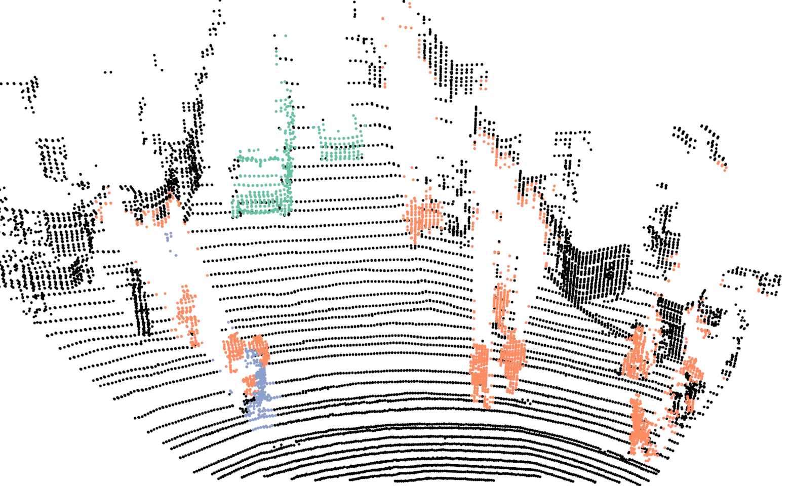 Figure 1
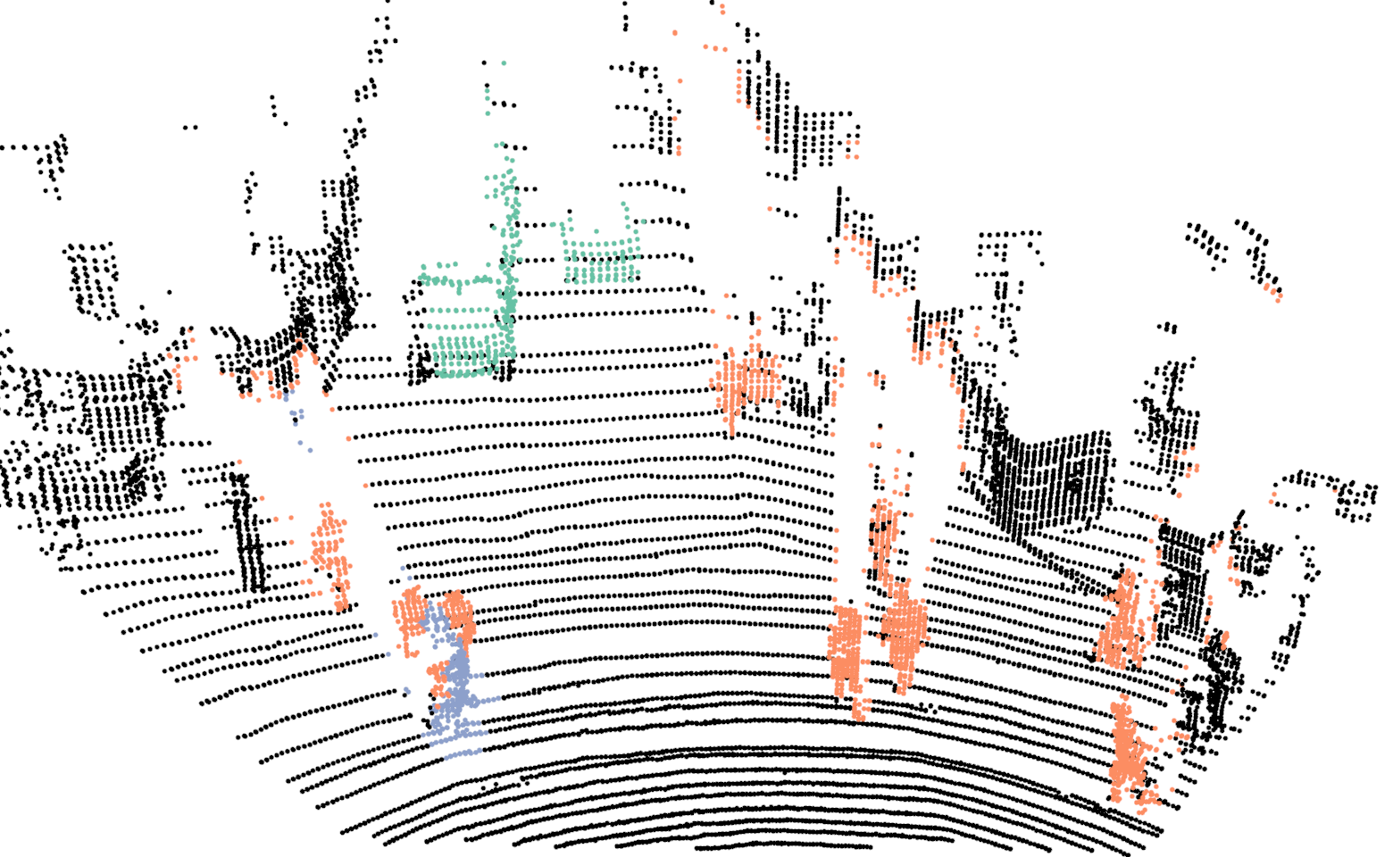 Figure 2
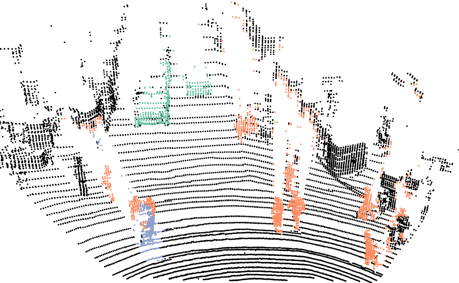 Figure 3
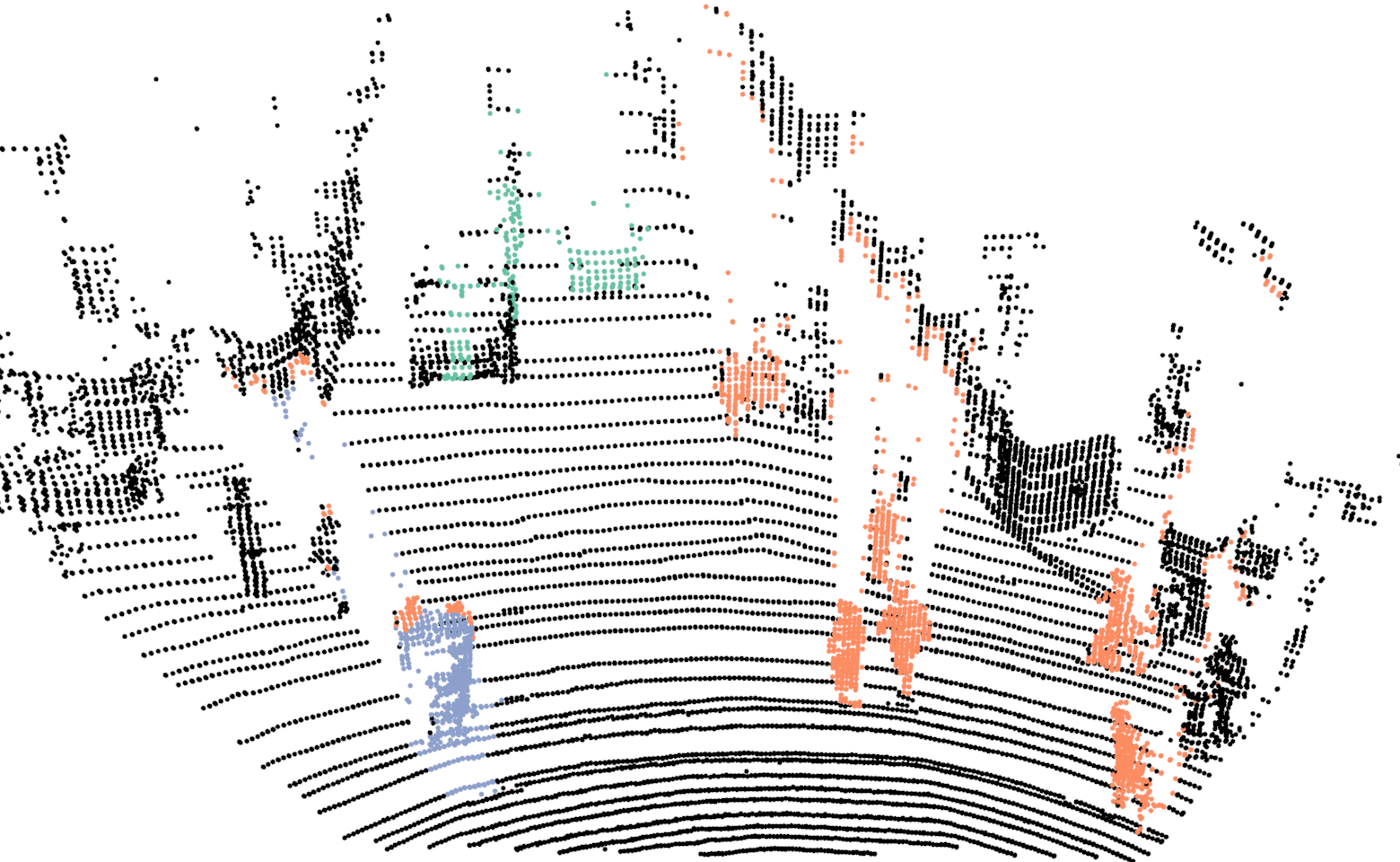 Figure 4
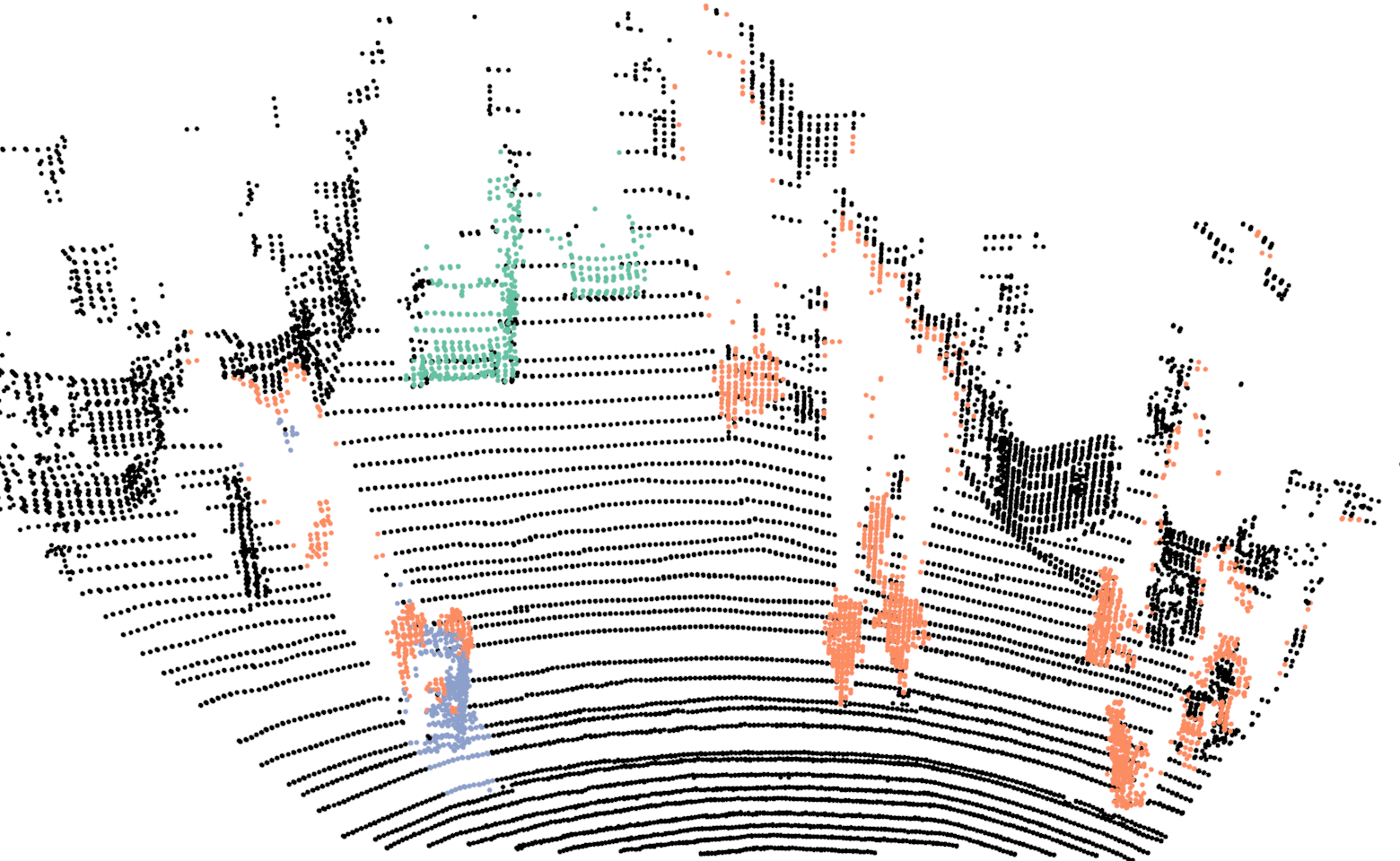 Figure 5
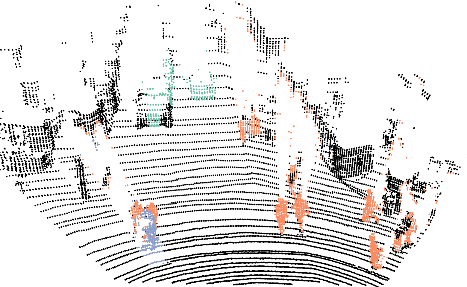 Figure 6
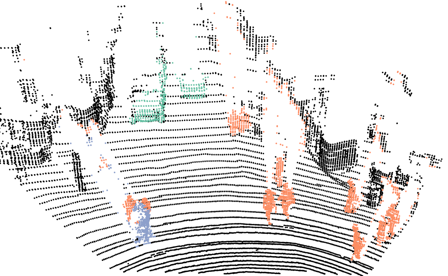 Figure 7
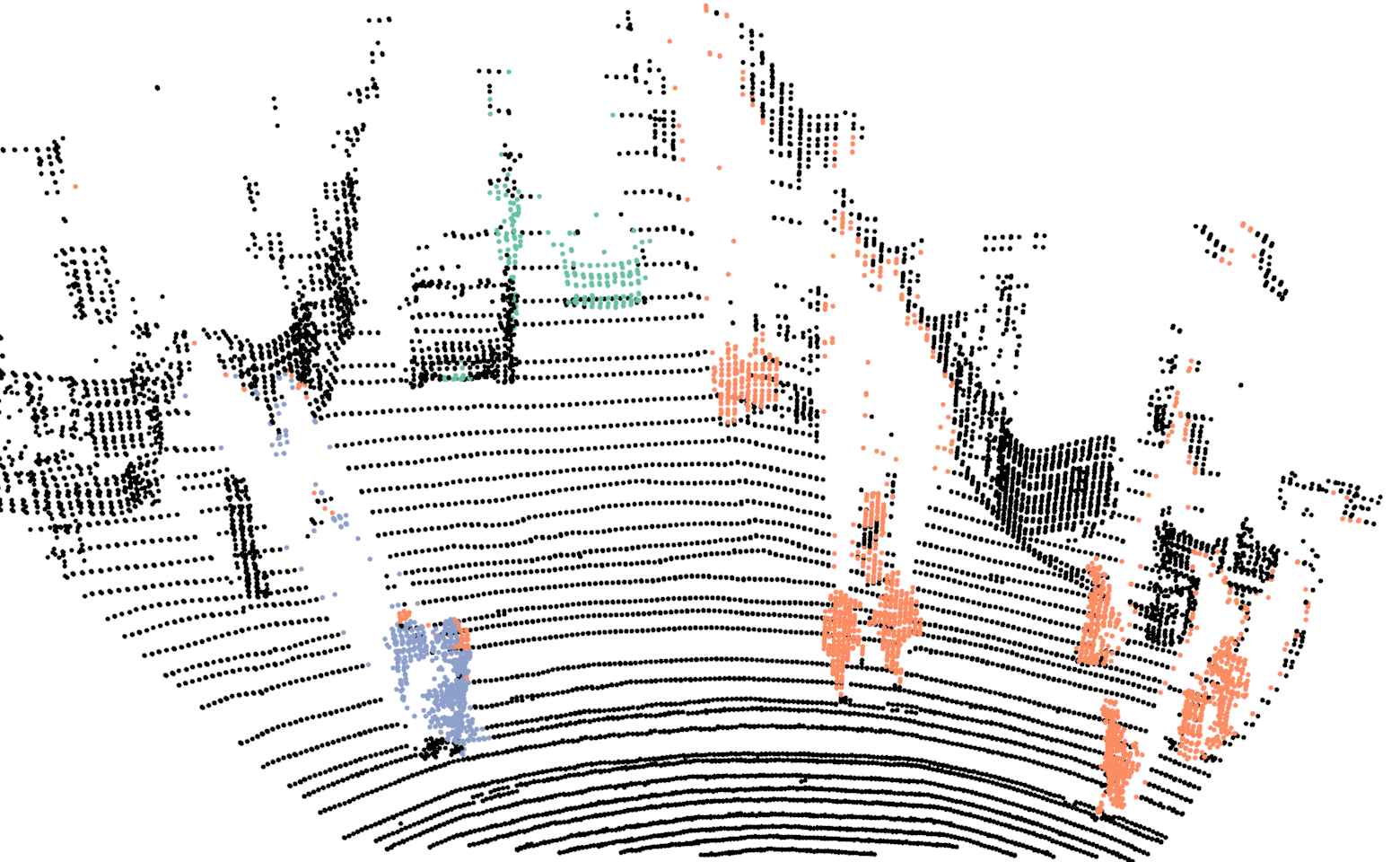 Figure 8
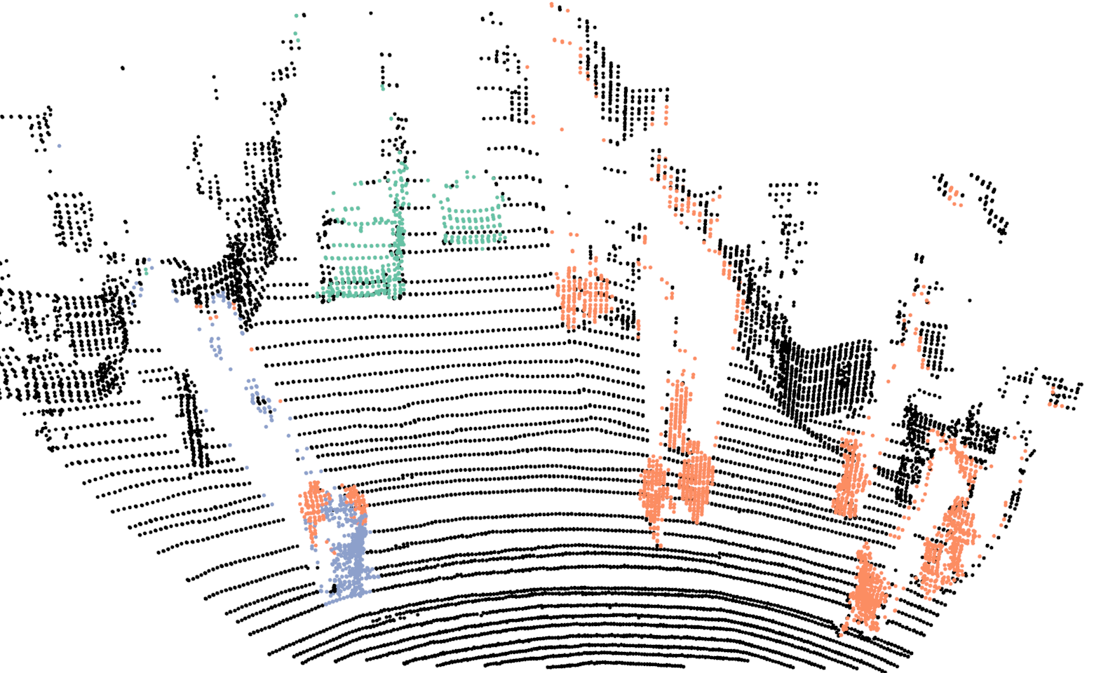 Figure 9
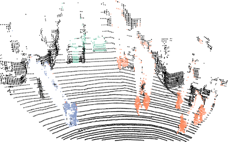 Figure 10
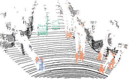 Figure 11
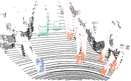 Figure 12
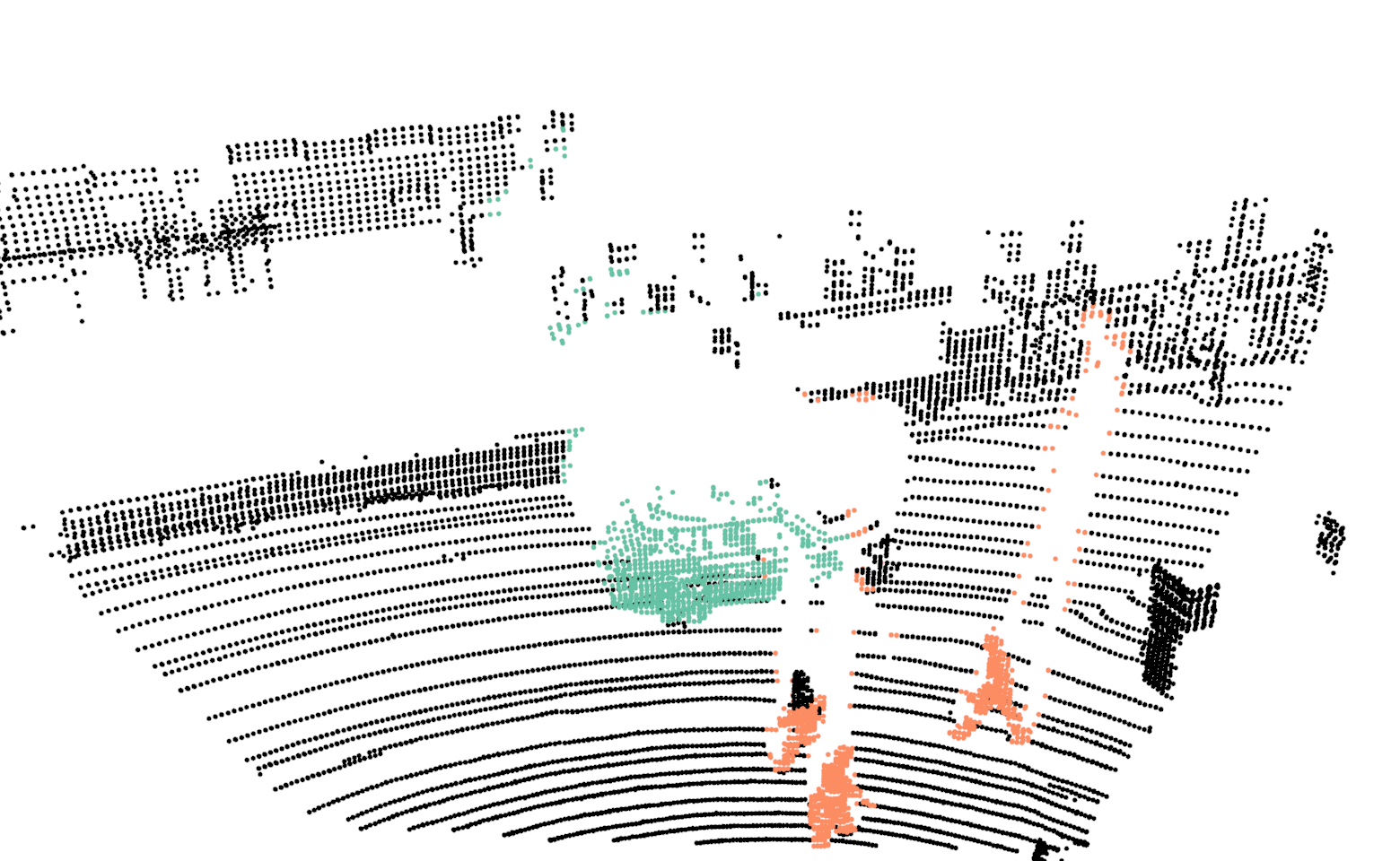 Figure 13
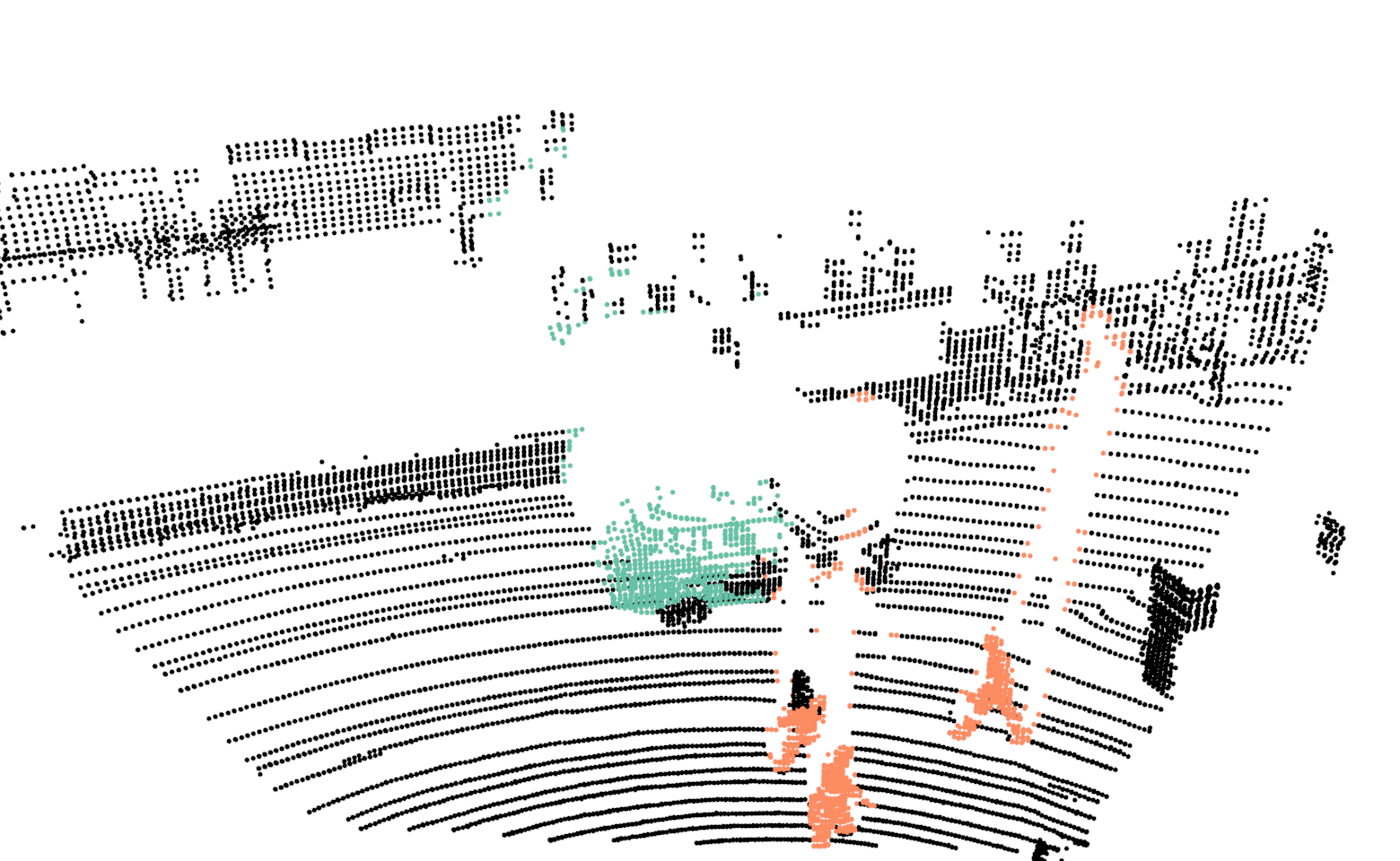 Figure 14
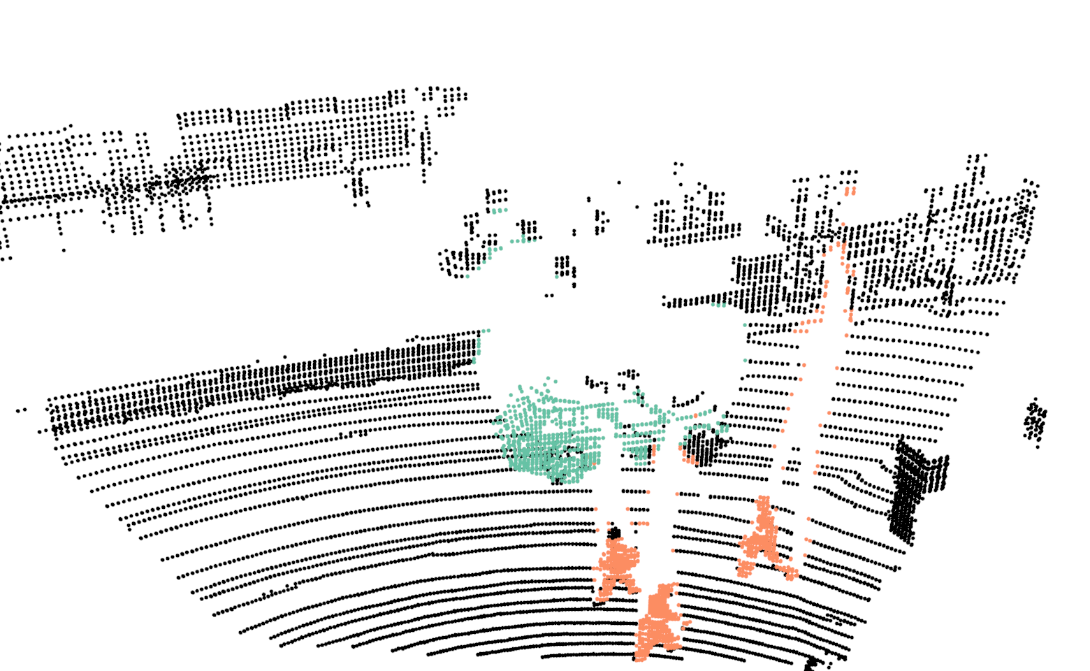 Figure 15
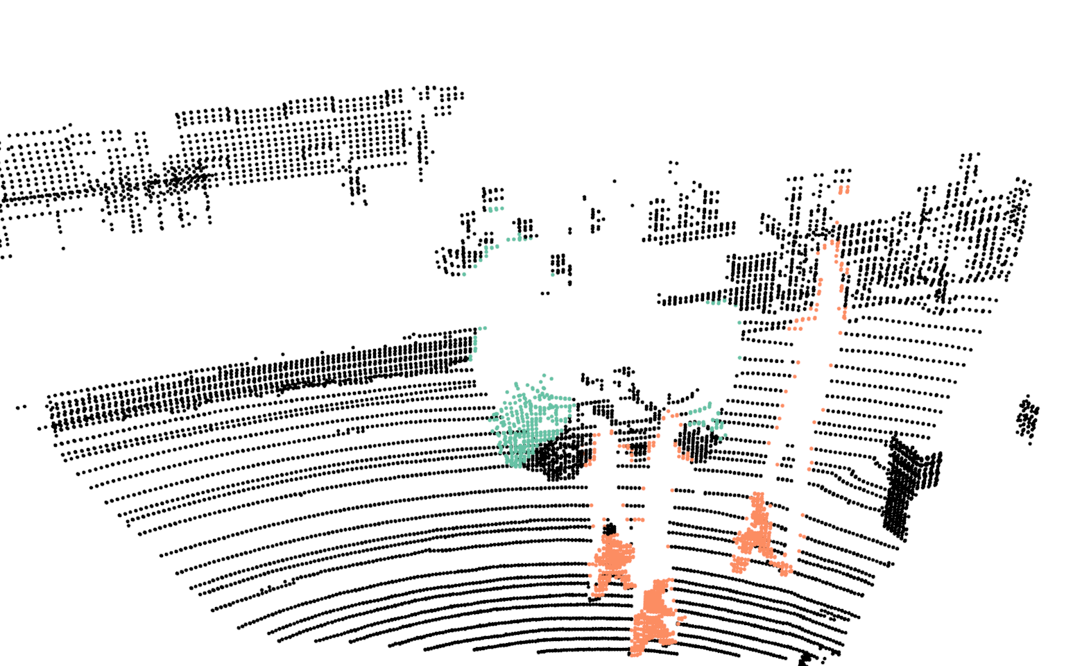 Figure 16
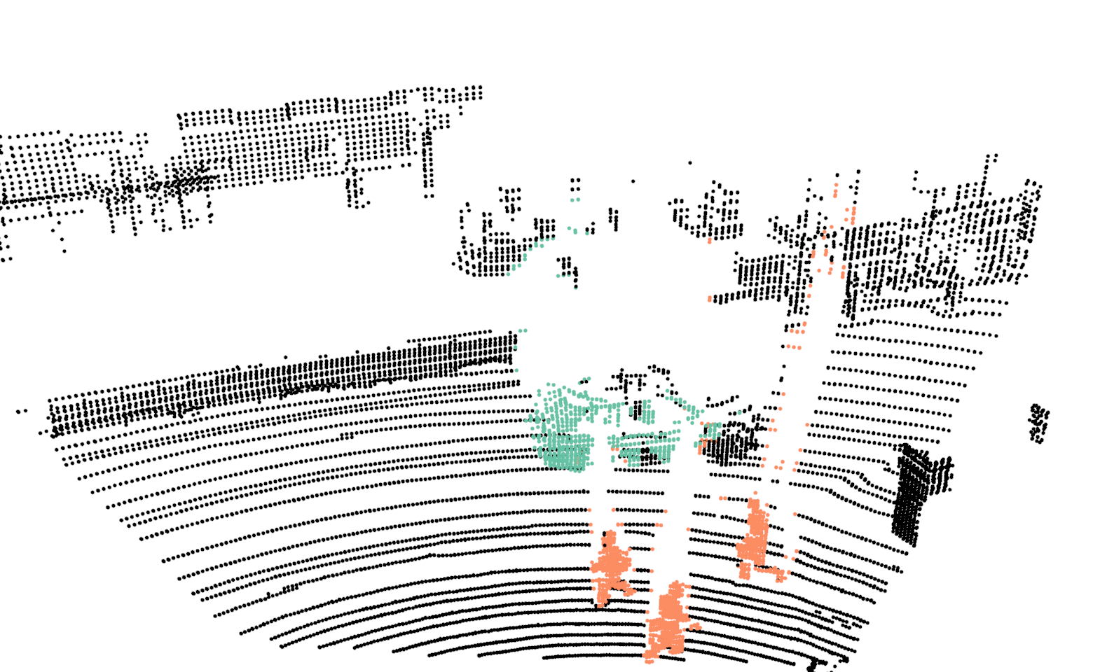 Figure 17
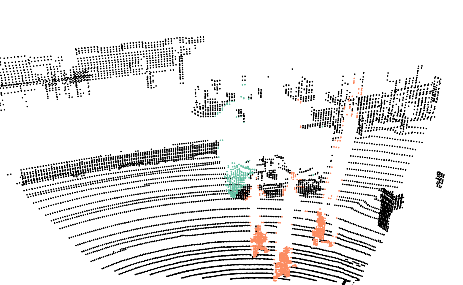 Figure 18
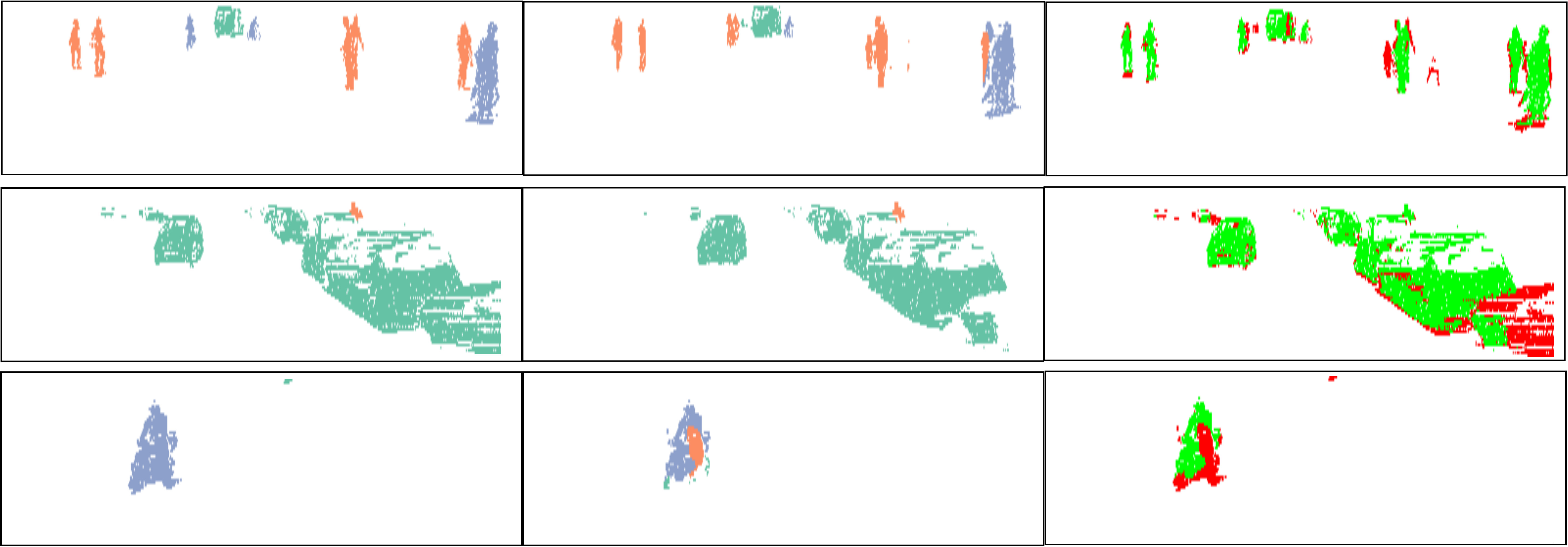 Figure 19
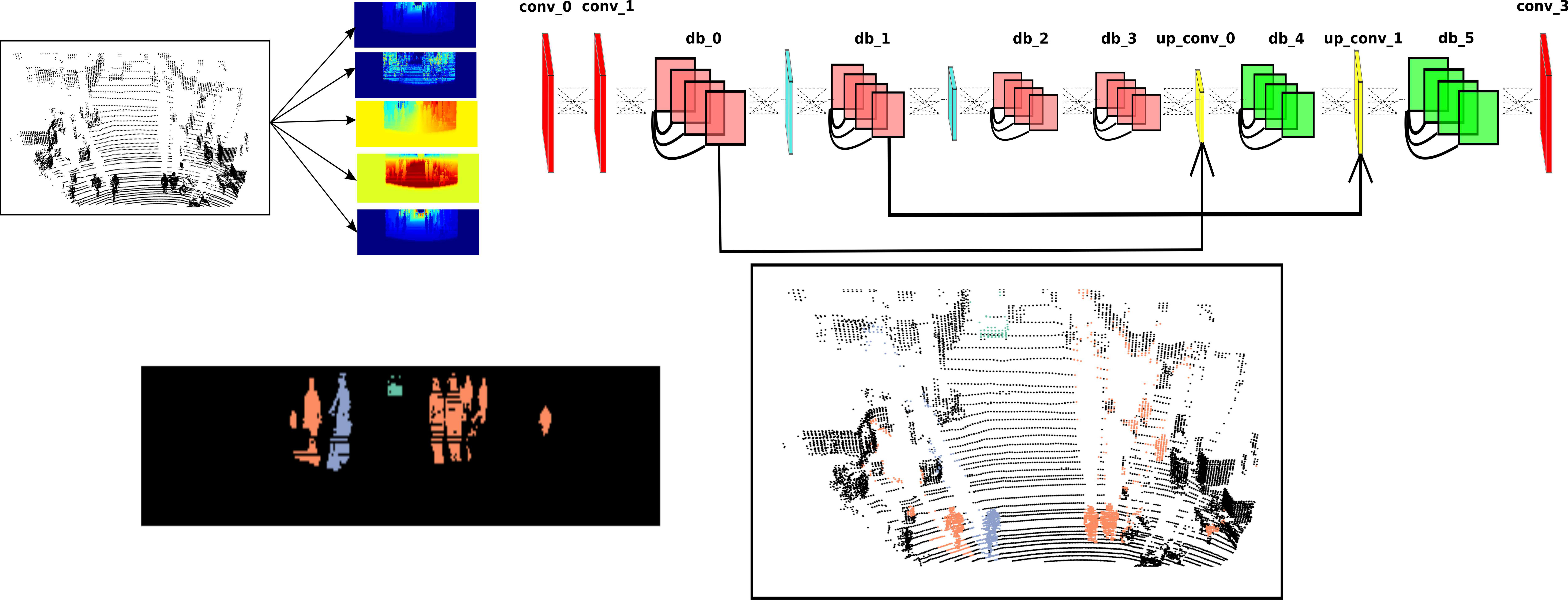 Figure 20
| Layer name | Dimension (HWC) | Repetition | Depth separable |
| conv_0 | - | No | |
| conv_1 | - | No | |
| db_0 | 6 | No | |
| db_1 | 8 | No | |
| db_2 | 10 | No | |
| db_3 | 15 | Yes | |
| up_conv_0 | - | No | |
| db_4 | 8 | Yes | |
| up_conv_1 | - | No | |
| db_5 | 6 | Yes | |
| conv_2 | - | No |
| Method | Cars | Pedestrians | Bicyclists | meanIoU |
| 100 Layer Tiramisu [13] | 74.2 | 48.7 | 43.7 | 55.5 |
| TD block [13] | 72.2 | 48.3 | 41.2 | 53.9 |
| Down-sample 8 | 74.1 | 43.8 | 39.7 | 52.5 |
| Down-sample width | 74.7 | 45.0 | 38.6 | 52.8 |
| db_3 depth separable | 74.2 | 49.2 | 36.8 | 53.4 |
| db_3 + db_2 depth separable | 73.6 | 41.2 | 33.2 | 49.3 |
| DBLiDARNet | 75.1 | 47.4 | 45.4 | 56.0 |
| Approach |
mIoU |
road |
sidewalk |
parking |
other-ground |
building |
car |
truck |
bicycle |
motorcycle |
other-vehicle |
vegetation |
trunk |
terrain |
person |
bicyclist |
motorcyclist |
fence |
pole |
traffic sign |
| PointNet [19] | 14.6 | 61.6 | 35.7 | 15.8 | 1.4 | 41.4 | 46.3 | 0.1 | 1.3 | 0.3 | 0.8 | 31.0 | 4.6 | 17.6 | 0.2 | 0.2 | 0.0 | 12.9 | 2.4 | 3.7 |
| SPGraph [15] | 17.4 | 45.0 | 28.5 | 0.6 | 0.6 | 64.3 | 49.3 | 0.1 | 0.2 | 0.2 | 0.8 | 48.9 | 27.2 | 24.6 | 0.3 | 2.7 | 0.1 | 20.8 | 15.9 | 0.8 |
| SPLATNet [24] | 18.4 | 64.6 | 39.1 | 0.4 | 0.0 | 58.3 | 58.2 | 0.0 | 0.0 | 0.0 | 0.0 | 71.1 | 9.9 | 19.3 | 0.0 | 0.0 | 0.0 | 23.1 | 5.6 | 0.0 |
| PointNet++ [20] | 20.1 | 72.0 | 41.8 | 18.7 | 5.6 | 62.3 | 53.7 | 0.9 | 1.9 | 0.2 | 0.2 | 46.5 | 13.8 | 30.0 | 0.9 | 1.0 | 0.0 | 16.9 | 6.0 | 8.9 |
| SqueezeSeg [27] | 29.5 | 85.4 | 54.3 | 26.9 | 4.5 | 57.4 | 68.8 | 3.3 | 16.0 | 4.1 | 3.6 | 60.0 | 24.3 | 53.7 | 12.9 | 13.1 | 0.9 | 29.0 | 17.5 | 24.5 |
| SqueezeSegV2 [28] | 39.7 | 88.6 | 67.6 | 45.8 | 17.7 | 73.7 | 81.8 | 13.4 | 18.5 | 17.9 | 14.0 | 71.8 | 35.8 | 60.2 | 20.1 | 25.1 | 3.9 | 41.1 | 20.2 | 36.3 |
| TangentConv [25] | 40.9 | 83.9 | 63.9 | 33.4 | 15.4 | 83.4 | 90.8 | 15.2 | 2.7 | 16.5 | 12.1 | 79.5 | 49.3 | 58.1 | 23.0 | 28.4 | 8.1 | 49.0 | 35.8 | 28.5 |
| DarkNet21Seg | 47.4 | 91.4 | 74.0 | 57.0 | 26.4 | 81.9 | 85.4 | 18.6 | 26.2 | 26.5 | 15.6 | 77.6 | 48.4 | 63.6 | 31.8 | 33.6 | 4.0 | 52.3 | 36.0 | 50.0 |
| DarkNet53Seg | 49.9 | 91.8 | 74.6 | 64.8 | 27.9 | 84.1 | 86.4 | 25.5 | 24.5 | 32.7 | 22.6 | 78.3 | 50.1 | 64.0 | 36.2 | 33.6 | 4.7 | 55.0 | 38.9 | 52.2 |
| DBLiDARNet | 37.6 | 85.8 | 59.3 | 8.7 | 1.0 | 78.6 | 81.5 | 6.6 | 29.4 | 19.6 | 6.5 | 77.1 | 46.0 | 58.1 | 23.7 | 20.1 | 2.4 | 39.6 | 32.6 | 39.1 |
| Seq. ID | DBLiDARNet | Object Bayes Filter | ||||
| Cars | Pedestrians | Bicyclist | Cars | Pedestrians | Bicyclist | |
| 0 | 76.2 | 2.0 | 29.6 | 79.2 | 2.0 | 23.6 |
| 2 | 54.9 | 37.0 | 0.0 | 55.3 | 46.9 | 0.0 |
| 3 | 75.2 | - | - | 75.5 | - | - |
| 4 | 66.6 | 40.8 | 35.2 | 69.1 | 47.4 | 53.2 |
| 5 | 70.1 | - | - | 70.0 | - | |
| 6 | 87.2 | - | - | 87.1 | - | - |
| 7 | 83.2 | 28.2 | - | 83.5 | 32.7 | - |
| 8 | 66.9 | - | - | 69.9 | - | - |
| 9 | 71.9 | 18.6 | - | 72.9 | 21.6 | - |
| 10 | 72.4 | 0.0 | 0.0 | 75.1 | 0.0 | 0.0 |
| 11 | 88.4 | 15.6 | - | 89.6 | 15.3 | - |
| 12 | 51.5 | 0.0 | 4.0 | 58.5 | 0.0 | 1.6 |
| 13 | 24.2 | 50.7 | 39.5 | 31.3 | 50.6 | 41.1 |
| 14 | 89.6 | 40.2 | - | 86.3 | 42.6 | - |
| 15 | 83.9 | 70.1 | 5.0 | 85.7 | 72.5 | 5.0 |
| 16 | 63.8 | 75.3 | 54.5 | 64.1 | 77.0 | 60.7 |
| 17 | - | 81.8 | 0.0 | - | 83.7 | 0.0 |
| 18 | 84.7 | - | - | 84.7 | - | - |
| 19 | 68.4 | 66.2 | 36.9 | 74.0 | 66.1 | 37.8 |
| 20 | 69.1 | - | - | 69.4 | - | - |
Peer Reviews
No public reviews on file for this paper yet. If you reviewed it on a platform where reviews are public (OpenReview, ICLR, NeurIPS, ICML), you can paste yours below so the community can read it here.
Code & Models
Videos
No videos yet. Explain this paper in a talk, walkthrough, or lecture? Add one.
Taxonomy
MethodsDiffusion-Convolutional Neural Networks
DeepTemporalSeg: Temporally Consistent Semantic Segmentation of 3D LiDAR Scans
Ayush Dewan1
Wolfram Burgard1,2 1Department of Computer Science, University of Freiburg, Germany.2Toyota Research Institute, Los Altos, USA.
Abstract
Understanding the semantic characteristics of the environment is a key enabler for autonomous robot operation. In this paper, we propose a deep convolutional neural network (DCNN) for semantic segmentation of a LiDAR scan into the classes car, pedestrian and bicyclist. This architecture is based on dense blocks and efficiently utilizes depth separable convolutions to limit the number of parameters while still maintaining the state-of-the-art performance. To make the predictions from the DCNN temporally consistent, we propose a Bayes filter based method. This method uses the predictions from the neural network to recursively estimate the current semantic state of a point in a scan. This recursive estimation uses the knowledge gained from previous scans, thereby making the predictions temporally consistent and robust towards isolated erroneous predictions. We compare the performance of our proposed architecture with other state-of-the-art neural network architectures and report substantial improvement. For the proposed Bayes filter approach, we shows results on various sequences in the KITTI tracking benchmark.
I Introduction
In the last decade, the research towards self-driving cars has picked up a staggering pace. The main objective of this technology is to make our roads safer than ever before [1]. A key ingredient to realize the goals of autonomous vehicles is a robust perception system, where the main objective is to understand the environment in which the robot is operating, through a variety of sensors that a robot is endowed with. In this paper, we focus of semantic scene understanding of urban outdoor environment using 3D LiDAR scans. Semantic understanding is crucial, as it paves the way for robust visual localization [18, 21], efficient mapping [23], among several other tasks.
In this paper, we propose a deep convolutional neural network (DCNN) architecture for the task of semantic segmentation of a 3D LiDAR scan into the following semantic categories: car, pedestrian and bicyclist. Our proposed architecture is based on dense blocks [11]. To reduce the number of parameters, we replace the standard convolution layers with depth separable convolution layers [7] for dense blocks in the decoder. This allows us to reduce the number of parameters by a significant amount while still having competitive performance.
Standard DCNN architectures treat each example independently and do not use any previous or prior information. Especially in the case of perception in robotics, the data is sequential. To leverage over this sequential nature of information, we propose a Bayes filter approach for making our segmentation results temporally consistent. More concretely, we use a Bayes filter with a static state, where static in this context means that transition between different states is unlikely, which is true for semantic classes. This approach neatly combines the current prediction of the neural network, with the information accumulated from previous scans. In our previous work [9], such an approach was part of our method to classify points in a 3D LiDAR scan as non-movable, movable and dynamic. We illustrated its advantages through qualitative results. In this paper, we thoroughly analyze our method by evaluating our approach on various sequences of KITTI tracking benchmark and report both qualitative and quantitative results.
The main contributions of this paper include a DCNN for semantic segmentation of LiDAR scans into the classes: car, pedestrian and bicyclist. We compare our DCNN with state-of-the-art DCNNs [27, 28, 26], proposed for the same task. To justify different architecture design choices and gain further insight towards them, we also present an ablation study. Our next contribution is a Bayes filter approach for making the predictions of the neural network temporally consistent. This approach leverages over the sequential nature of the input data stream and makes our segmentation system robust towards sporadic erroneous prediction. For comparison, we use our proposed architecture as a baseline method. The code for the proposed architecture, along the trained model and the dataset is available here http://deep-temporal-seg.informatik.uni-freiburg.de/.
II Related Work
With the advent of deep neural networks, a significant progress has been made towards solving a variety of tasks, including the task of semantic segmentation. Regarding 2D images, a plethora of research has been done in last few years [17, 22, 3, 13, 5], pushing the boundary of state-of-the-art results to the limit. A similar progress has not been in the field of semantic segmentation of 3D pointcloud data due to inherent differences in the two data modalities. In the case of 2D images, the input data to the network is fixed but in the case of 3D data, multiple representations are possible. Regarding the current task, the most commonly used representation are either a collection of 3D points or projecting the pointcloud on a 2D image. For the first representation, the PointNet and PointNet++ architecture proposed by Qi et al. [19, 20] is a popular choice for learning from unordered pointcloud. They have shown results primarily on indoor sequence for the data collected from RGB-D sensors. In our case, we use a LiDAR scanner for segmentation of urban outdoor environments. The data from LiDAR scanner is sparser in comparison to the RGB-D sensor and the outdoor environment is more spread out in comparison to confined indoor spaces. In our case, we use the second representation i.e. projecting the 3D LiDAR scan on to a 2D image. This allows us to represent a LiDAR scan in a compact fashion and furthermore the advancements made in the field of semantic segmentation using 2D images can be used as well.
Focusing on the task of semantic segmentation using 2D images, one of the initial architectures was proposed by Long et al. [17]. They proposed an encoder-decoder style, fully convolutional network (FCN) architecture and other architectures since then have followed the same paradigm. Jégou et al. [13] proposed a dense block based DCNN for the task of semantic segmentation. The main differences between our DCNN and theirs is that we use depth separable convolution layers for dense blocks in the decoder. To down-sample the feature maps they proposed a transition down block comprising of a composite function implementing different operations. We replace this block with a single max-pooling operation and show that instead of a composite function, this single operation is sufficient. In the presented ablation study, we justify these proposed changes.
We compare our proposed architecture with the architectures proposed in [27, 28, 26]. The first architecture proposed by Wu et al. [27] is based on the SqueezeNet [12] architecture. They use fire modules, which first involves squeezing the feature maps using filters and then expanding these squeezed feature maps in parallel using filters of size and and concatenating their outputs at the end. Using three max-pool layers they down-sample the feature maps only along the width dimension and to up-sample the feature maps they again use fire modules in the decoder. Last layer of their neural network architecture is a recurrent CRF and the complete architecture is trained end-to-end. In our ablation study, we compare with their proposed down-sampling technique.
They further improve this architecture in [28] by using a binary mask as an additional input channel. This mask indicates existence of a LiDAR measurement corresponding to a pixel location. Along this they also introduce a novel context aggregation module to limit the error introduced by missing LiDAR measurements and furthermore in order to tackle the class imbalancing problem they use focal loss [16] for training their DCNN. The last method we compare with is the DCNN proposed by Wang et al. [26]. Similar to the neural network architectures proposed by Wu et al. [27], their network architecture is also based on SqueezeNet. They also use Squeeze Excitation blocks [10] after the initial fire modules and at the end of the encoder use an enlargement layer which is based on the Atrous Spatial Pyramid Pooling [6].
III Network Architecture
In Fig.2 we illustrate the complete framework for semantic segmentation of a LiDAR scan. The first step is to project the scan onto different 2D images and each such image encodes a specific modality. These images are then stacked together and are passed through our proposed DCNN for semantic segmentation. The segmentation mask predicted by the DCNN is then projected back to the LiDAR scan to infer pointwise semantic labels.
For the task of semantic segmentation we a propose a novel fully convolutional DCNN architecture called DBLiDARNet. Our architecture is based on dense blocks and is shown in Fig.2. Similar to other DCNN architecture proposed for the task of semantic segmentation [13, 17, 22], our network is also comprised of an encoder for learning the features required for the task while down-sampling the feature map size and a decoder to up-sample the feature maps so that the last hidden layer has the same spatial resolution as the input image. In the encoder, we have two convolution layers (conv_0 and conv_1), four dense blocks (db_0, db_1, db_2 and db_3) and two max-pooling layers to down-sample the feature maps in comparison to the spatial resolution of the input image. In the decoder we use two up-convolution layers to up-sample the feature maps and use two more dense blocks with depth separable convolution layers. To limit the number of learnable parameters in the decoder, similar to the architecture proposed by Jégou et al. [13], in our proposed architecture the input to the up-convolution layers is the feature maps learned by the dense block prior to the up-convolution layer instead of all the features maps learned till that point. For instance the input to the layer up_conv_0 is only the feature maps learned by the dense block db_3. To recapture the information lost during up-sampling we use skip connections to concatenate the feature maps from the encoder to the output of the up-convolution layers. The complete details regarding the dimensions of each layer or block and different associated hyper-parameters is reported in Tab.I.
III-A Training
Our complete network architecture is implemented in TensorFlow [2]. We use the dataset provided by Wu et al. [27]. We use softmax cross-entropy loss and use the Adam optimizer [14] with a learning rate of , weight decay of and batch size of . Among the three classes, the point measurements from cars is significantly more than the measurements from either pedestrians or bicyclists, mainly because of the inherent difference in the size of the geometrical structure. This leads to the problem of class imbalancing, where some classes in the training data overwhelm the classes which are under represented. To tackle this we use a weight balancing technique and assign larger weights to points belonging to the class pedestrian and bicyclist in comparison to points belonging to the class car and background.
IV Bayes Filter Method
In the Sec.III, we proposed a novel DCNN architecture for semantic segmentation of a LiDAR scan into different categories. The output of the network is the predicted softmax probabilities of a point in a scan belonging to different categories. Since this prediction is performed independently for different scans, in this section we introduce a novel Bayes Filter approach to make our pointwise prediction temporally consistent. This approach assumes the scans are sequential with significant overlap and the objective is to leverage over this sequential nature of information and make our prediction robust to isolated erroneous predictions from the neural network.
The semantic state of a point is static, i.e. it remains same over time and transition between these states is unlikely. For each point, we use three separate binary Bayes filters with static state, to estimate the belief for each class independently. To estimate the belief for a class , for a point in a scan at time , we first define a binary random state variale , where indicates that the point belongs to the class and indicates the opposite. Without loss of generality, from now on, we would write as and as . The current belief depends only on the predictions of the neural network, , for the class as shown in Eq.(1).
[TABLE]
where, are softmax scores for the class . We define such binary random variables for each class and estimate the belief for each class independently. Using Bayes rule and Markov assumption we can rewrite the Eq.(1) as following,
[TABLE]
Using Bayes rule for the term , Eq.(2) can be modified as following,
[TABLE]
Similarly, can be written as,
[TABLE]
We now introduce the log odds notation, where odds of an event is defined in Eq.(5) and the log odds are defined in Eq.(6)
[TABLE]
The odds for a point having the semantic class can be estimated by dividing Eq.(3) with Eq.(4). The odds is defined in Eq.(7) and the log odds are defined in Eq.(9),
[TABLE]
where, the current measurement is defined as following,
[TABLE]
In Eq.(9), are the log odds for the belief at time , the first term on the right side in Eq.(9) are the log odds for the current measurement, are the log odds for the previous belief and are the log odds for the initial belief. Through this formulation, our inference not only depends on the current measurement (), but also on the previous measurements, incorporated through the recursive term . To enable this recursive behavior, data association between points in consecutive scans is required and for this we use our method of estimating pointwise motion proposed in [8]. We perform data association by aligning scans using the estimated motion and choosing the nearest point on the basis of Euclidean distance as the corresponding point. As mentioned before, we estimate for each class separately and for the inference we choose the class with the largest odds.
V Results
V-A Network Architecture
To evaluate our proposed DCNN, we use the test set from the dataset provided by Wu et al. [27]. We report class wise IoU and compare our results with two DCNN proposed by Wu et al. ([27],[28]) and the network architecture proposed by Wang et al. [26]. In Fig.3, we show qualitative semantic segmentation results. In Tab.II we report the class wise IoU and mean IoU for different methods. Our proposed DCNN outperforms the existing state-of-the art DCNNs proposed for the same task and has a better IoU for all the three classes. In the case of pedestrian, the increase in IoU is around 70%, for the class bicyclist the increase is around 17%, with an overall increase in mean IoU by 16%. These results indicate a remarkable improvement over the existing DCNNs proposed to solve the same task. Comparing the inter class performance, the highest IoU is achieved for the class car, whereas the performance for pedestrian and bicyclist are comparable. Similar trend is evident for other methods as well. This difference in performance has three main reasons, firstly the number of instances of pedestrian and bicyclist is lesser in comparison to car. Secondly, object in both these classes have a smaller size in comparison to cars and therefore the number of points sampled from their surface is significantly lower in comparison to points sampled from the surface of cars. Due to these reasons, these two classes are under represented and as mentioned before, we use weight balancing in order to have a large penalty for misclassifying points in these classes. The last reason is the over segmentation of points on a bicyclist into classes bicyclist and pedestrian as shown in Fig.3. This misclassification is not a common occurrence but still hampers the overall performance.
V-A1 Ablation Study
In this ablation study, we justify the network design choices we mentioned in Sec.III. The main differences between our dense blocks based fully convolutional network and the architecture proposed by Jégou et al. [13].
Replacing the transition-down block with max pooling for down-sampling the feature maps. This block implements a composite function comprising of batch normalization, ReLU activation, convolution layer (), dropout and max-pooling. We replace this transition-down block by a max-pooling layer. This decision is based on our empirical findings. 2. 2.
Using depth separable convolution layers instead of convolution layers for dense blocks in the decoder. This helps in reducing the parameters from 3.6M to 2.8M.
The architecture proposed by Jégou et al. [13] consists of five transition down blocks for down-sampling the feature maps 32. They, therefore use five up-convolution layers in the decoder along with same number of dense blocks. Such a high down-sampling rate will result in significant loss of information for reasons discussed before (Sec.III). Therefore in our implementation of their architecture we only use two transition down blocks instead of five. In Tab.III we report results for a model where we use our architecture but replace max-pool layers with transition down (TD) blocks. Our proposed architecture outperforms their architecture marginally while using fewer parameters. Using transition down blocks instead of a max-pooling layer leads to a slight decrease in performance as well. Comparing different down-sampling strategies, we trained two different models. For the first model we down-sample 8 instead of 4 and for the second model we down-sample 4 but only along the width dimension while keeping the height unchanged, similar to [27]. As reported in Tab.III, for the first model (down-sample 8), the IoU for the class car remains comparable but a decrease in performance is observed for the other classes. In comparison to cars, pedestrians and bicyclists are smaller and therefore a large down-sampling rate adversely affects these classes in comparison to other classes. For the second model, similar to the first, a noticeable decrease in performance is observed for both pedestrian and bicyclist classes. Without decreasing the height, feature maps have larger spatial resolution, thereby requiring more operations. Even though large down-sampling rate can hamper the performance, especially for the task of semantic segmentation, it is still required for increasing the receptive field as well as making the model efficient considering both the memory and computational requirements. Our proposed strategy of down-sampling the feature maps 4 allows us to exploit the advantages of such operations without losing the crucial information necessary for predicting accurate segmentation masks.
We trained two models, where we use depth separable convolution only in the last dense block of the encoder (db_3) and then in last two dense blocks together (db_3 + db_2). In both cases performance decreases, especially for the second case the decrease is substantial. Even though depth separable convolution is an ingenious way of reducing parameters but excessively using it can decrease performance as well.
V-A2 Semantic KITTI
In Tab.IV, we report results for the semantic KITTI dataset [4].
V-B Bayes Filter
To evaluate our proposed Bayes filter approach, we use the KITTI tracking benchmark. The benchmark contains 20 sequences and to evaluate our approach on all of the sequences, we split the sequences into two different sets. We train our network on both sets separately and use the other set for testing i.e. we train a model on the first set and test the learned model on the second set and then train on the second set and test on the first set.
For training the network we use our proposed network with the exact same parameters as discussed in Sec.III-A, with the one difference. In this case the input resolution of the images are , in comparison to . For evaluating the proposed Bayes filter we use our network as the baseline method and report comparison with the segmentation results from the network. In Fig.4, we illustrate the differences in the segmentation results for a sequence of six consecutive scans. In the case of neural network, points on a car are correctly classified in the first scan but in the next few scans, points on the same car are misclassified as background. For the same scans, our proposed Bayes filter is able to consistently classify points on the car correctly.
In Tab.V, we report class wise IoU for different sequences, for both our DCNN and the Bayes filter approach. In the cases where no instances of a class is observed, we do not report results as well (indicated by a dash sign). The performance of our DCNN on this dataset is similar to the results reported in Sec.V. For some sequences, the IoU for the class bicyclists is zero. In these cases, majority of times these objects are either far from the sensor or occluded and in the rare cases they are misclassified as pedestrians.
Comparing the DCNN results with the Bayes filter approach, across different sequences and classes, an improvement in IoU is consistently observed after using the Bayes filter approach. For most cases the improvement in IoU is around 4% to 9% but an improvement of 27% is achieved for class pedestrian in sequence 2 and staggering improvement of 51% is achieved for class bicyclist in sequence 4. For couple of isolated cases, a decrease in IoU is observed after using the filter approach. The implicit assumption of our Bayes filter approach is that the predictions from DCNN is seldom wrong and for cases, the filter uses the previous knowledge to correct those predictions. In the rare cases where this assumption is violated, the information accumulated by the filter spurs from incorrect measurements and therefore the filter approach needs multiple correct predictions from DCNN to improve its knowledge in comparison to a single prediction needed by DCNN. For instance, in the sequence 0, points on a bicyclist were labeled as pedestrian more than often, causing Bayes filter to accumulate the incorrect predictions.
VI Conclusions
In this paper, we proposed a DCNN to segment points in a 3D LiDAR scan into multiple semantic categories. Our proposed architecture is based on dense blocks and uses depth separable convolution to reduce the parameters while still maintaining competitive performance. It significantly outperforms state-of-the-art neural network architectures, with an average improvement of around 16% across different classes. In the presented ablation study, we justify our architecture choices. The neural network predicts the segmentation mask for each scan independently and to make these predictions temporally consistent, we proposed a Bayes filter method. Through extensive evaluation on the KITTI tracking benchmark, we report a consistent improvement across classes and sequences.
The reference list from the paper itself. Each links out to its DOI / PubMed record.
- 1way [2019] Waymo: Our Mission. https://waymo.com/mission/ , 2019. [Online; accessed 28-May-2019].
- 2Abadi et al. [2016] Martín Abadi, Ashish Agarwal, Paul Barham, Eugene Brevdo, Zhifeng Chen, Craig Citro, Greg S Corrado, Andy Davis, Jeffrey Dean, Matthieu Devin, et al. Tensorflow: Large-scale machine learning on heterogeneous distributed systems. ar Xiv preprint ar Xiv:1603.04467 , 2016.
- 3Badrinarayanan et al. [2015] Vijay Badrinarayanan, Alex Kendall, and Roberto Cipolla. Segnet: A deep convolutional encoder-decoder architecture for image segmentation. ar Xiv preprint ar Xiv: 1511.00561 , 2015. URL http://arxiv.org/abs/1511.00561 .
- 4Behley et al. [2019] J. Behley, M. Garbade, A. Milioto, J. Quenzel, S. Behnke, C. Stachniss, and J. Gall. Semantic KITTI: A Dataset for Semantic Scene Understanding of Li DAR Sequences. In Proc. of the IEEE/CVF International Conf. on Computer Vision (ICCV) , 2019.
- 5Chen et al. [2017] Liang-Chieh Chen, George Papandreou, Florian Schroff, and Hartwig Adam. Rethinking atrous convolution for semantic image segmentation. ar Xiv preprint ar Xiv:1706.05587 , 2017.
- 6Chen et al. [2018] Liang-Chieh Chen, George Papandreou, Iasonas Kokkinos, Kevin Murphy, and Alan L Yuille. Deeplab: Semantic image segmentation with deep convolutional nets, atrous convolution, and fully connected crfs. IEEE transactions on pattern analysis and machine intelligence , 40(4):834–848, 2018.
- 7Chollet [2017] François Chollet. Xception: Deep learning with depthwise separable convolutions. In Proceedings of the IEEE conference on computer vision and pattern recognition , pages 1251–1258, 2017.
- 8Dewan et al. [2016] Ayush Dewan, Tim Caselitz, Gian Diego Tipaldi, and Wolfram Burgard. Rigid scene flow for 3d lidar scans. In IEEE/RSJ International Conference on Intelligent Robots and Systems (IROS) , 2016.
