2D PET Image Reconstruction Using Robust L1 Estimation of the Gaussian Mixture Model
Azra Tafro, Damir Ser\v{s}i\'c, Ana Sovi\'c Kr\v{z}i\'c

TL;DR
This paper proposes a novel PET image reconstruction method using Gaussian mixture models and robust L1 estimation, improving resolution and reducing noise compared to traditional pixel-based approaches.
Contribution
It introduces a robust segmentation algorithm based on Gaussian mixture models and an iterative EM-like algorithm for PET image reconstruction.
Findings
Enhanced image resolution and noise robustness.
Reduced computational complexity and convergence time.
Demonstrated effectiveness on PET imaging data.
Abstract
An image or volume of interest in positron emission tomography (PET) is reconstructed from pairs of gamma rays emitted from a radioactive substance. Many image reconstruction methods are based on estimation of pixels or voxels on some predefined grid. Such an approach is usually associated with limited resolution of the reconstruction, high computational complexity due to slow convergence and noisy results. This paper explores reconstruction of PET images using the underlying assumption that the originals of interest can be modeled using Gaussian mixture models. A robust segmentation method based on statistical properties of the model is presented, with an iterative algorithm resembling the expectation-maximization algorithm. Use of parametric models for image description instead of pixels circumvent some of the mentioned limitations.
Click any figure to enlarge with its caption.
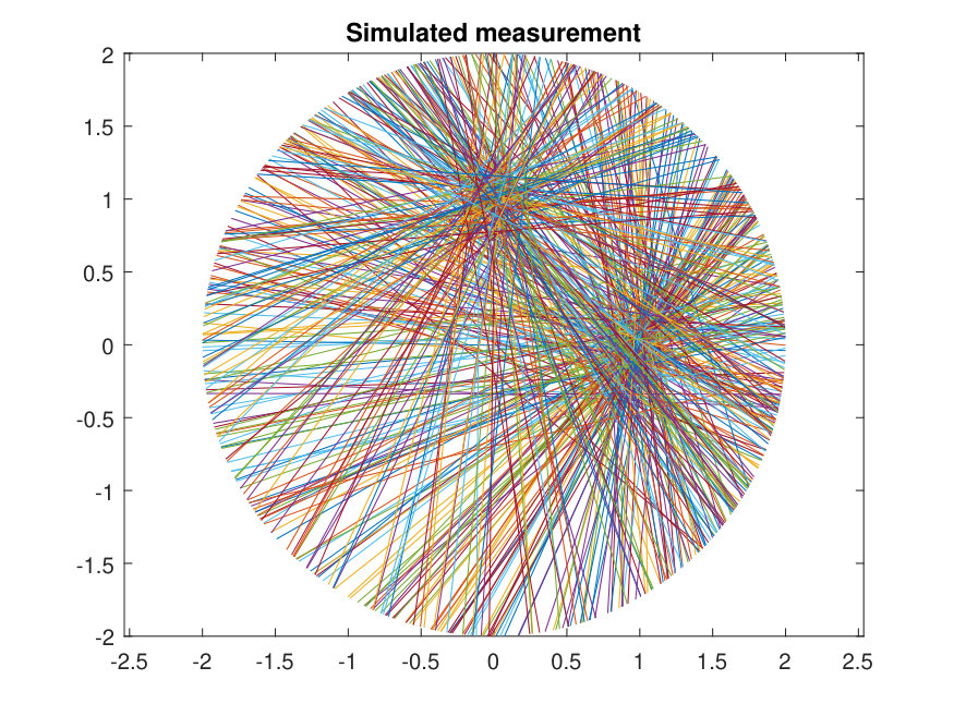 Figure 1
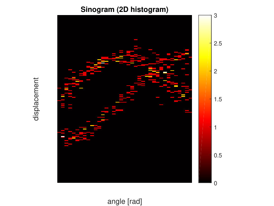 Figure 2
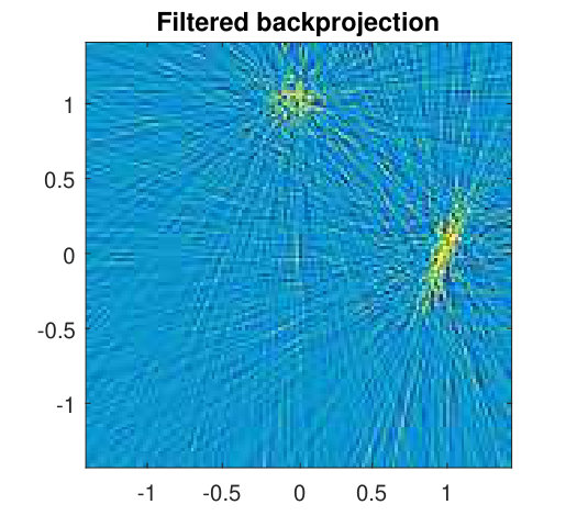 Figure 3
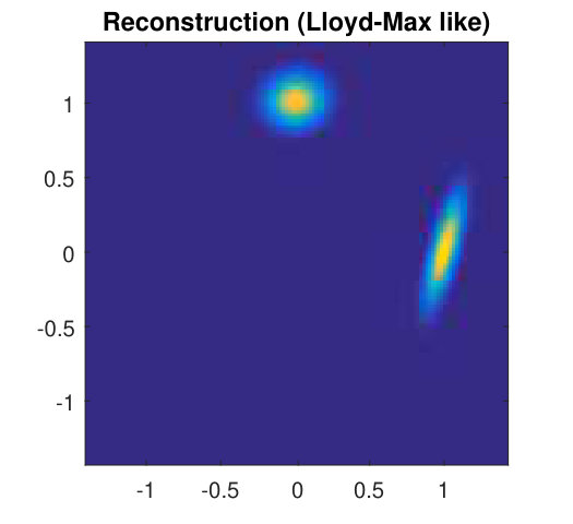 Figure 4
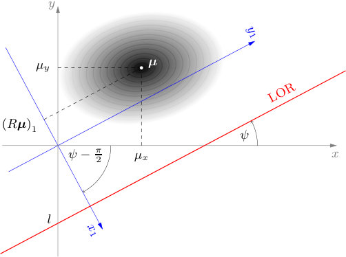 Figure 5
| method | 13.78% | 11.88% | 9.28% |
| method | 8.27% | 7.61% | 7.6% |
Peer Reviews
No public reviews on file for this paper yet. If you reviewed it on a platform where reviews are public (OpenReview, ICLR, NeurIPS, ICML), you can paste yours below so the community can read it here.
Videos
No videos yet. Explain this paper in a talk, walkthrough, or lecture? Add one.
Taxonomy
TopicsMedical Imaging Techniques and Applications · Bayesian Methods and Mixture Models · Statistical Methods and Inference
2D PET Image Reconstruction Using Robust Estimation of the Gaussian Mixture Model
††thanks: This work has been fully supported by Croatian Science Foundation under the project IP-2014-09-2625.
Azra Tafro, Damir Seršić and Ana Sović Kržić
Department of Electronic Systems and Information Processing
*University of Zagreb, Faculty of Electrical Engineering and Computing
*Zagreb, Croatia
[email protected], [email protected], [email protected]
Abstract
An image or volume of interest in positron emission tomography (PET) is reconstructed from pairs of gamma rays emitted from a radioactive substance. Many image reconstruction methods are based on estimation of pixels or voxels on some predefined grid. Such an approach is usually associated with limited resolution of the reconstruction, high computational complexity due to slow convergence and noisy results. This paper explores reconstruction of PET images using the underlying assumption that the originals of interest can be modeled using Gaussian mixture models. A robust segmentation method based on statistical properties of the model is presented, with an iterative algorithm resembling the expectation-maximization algorithm. Use of parametric models for image description instead of pixels circumvent some of the mentioned limitations.
Index Terms:
Gaussian mixture models, positron emission tomography, expectation-maximization (EM) algorithm, image segmentation
I Introduction
Positron emission tomography (PET) scanners detect the annihilation photon pairs arising from the positron emissions. Image reconstruction implies generating a two- or three-dimensional image of a radiotracer’s concentration to estimate physiologic parameters for volumes of interest in vivo. In three-dimensional scanners, we can consider the tube (parallelepiped) joining any two detector elements as a volume of response (VOR). In the absence of physical effects and noise, the total number of coincidence events detected will be proportional to the total amount of tracer contained in the volume of response. In the two-dimensional case, we consider only lines of response (LORs) joining two detector elements, lying within a specified imaging plane. The data are recorded as event histograms (sinograms or projected data) or as a list of recorded photon-pair events (list-mode data). For a general overview of standard PET image reconstruction methodology, see e.g. [1, 2] or [3].
Modern image reconstruction methods are mostly based on maximum-likelihood expectation-maximization (MLEM) iterations. Maximum likelihood is used as the optimization criterion, combined with the expectation-maximization algorithm for finding its solution. To overcome the computational complexity and slow convergence of the MLEM, the ordered subsets expectation-maximization (OSEM) algorithm has been recently introduced. Since MLEM or OSEM estimation of pixels or voxels is usually noisy [1], use of post-filtering methods is necessary. On the one hand, image reconstruction from its projections is a mature research field with well known methods and proven results. On the other hand, known limitations made a challenge for a different approach presented in this paper.
In image segmentation, a number of algorithms based on model-based techniques utilizing prior knowledge have been proposed to model uncertainty (see e.g. [4], [5]). The Gaussian mixture model (GMM) is a well-known and widely used model in a variety of segmentation and classification problems ([6],[7]).
In this paper, we propose a new robust algorithm for efficient reconstruction of an object from a PET image. Our method utilizes a novel minimizing algorithm to estimate the parameters of a Gaussian mixture model within framework similar to the standard expectation-maximization (EM) algorithm. Instead of voxels, we estimate parameters of the object’s model. We focus on the two-dimensional case for clarity, but an extension to three dimensions would follow in a similar fashion. This paper is organized into six sections. Section II gives an overview of traditional methodology in 2D PET imaging. In Section III an introduction to Gaussian mixture models is presented. Section IV describes the estimation of GMM parameters from PET data. Section V shows the implementation of iterative estimates in the EM-like algorithm. Finally, experimental results with discussion conclude the paper.
II Two-Dimensional PET Imaging
In the two-dimensional case, the acquired data are collected along LORs through a two-dimensional object. Traditionally, data are organized into sets of projections, integrals along all LORs for a fixed direction . The collection of all projections for forms a two dimensional function of the distance of the LOR from the origin, denoted by , and angle . The line-integral transform of is called the X-ray transform [8], which in 2D is the same as the Radon transform [9]. Since a fixed point traces a sinusoidal path in the projection space, the superposition of all sinusoids corresponding to each point of activity in a general object is called a sinogram. This is illustrated in Fig. 1.
A classical image reconstruction method is the filtered backprojection (FBP), which is based on the projection theorem of Fourier analysis. The algorithm reconstructs the image by calculating the inverse Fourier transform of the 2D Fourier transform of the backprojected image (see e.g. [2], [8], [10]). This technique does not include or depend on any assumptions about the data. Assumptions such as form, volume and dependence could be utilized to obtain more precise estimates.
III Gaussian Mixture Models
A Gaussian mixture model [11] is a weighted sum of component Gaussian densities as given by the equation:
[TABLE]
where is a -dimensional observation, are the weights of each Gaussian component, and are the Gaussian component densities. We assume that a given observation is a realization from exactly one of the Gaussian mixture components, and each component density is a -variate Gaussian function of the form:
[TABLE]
with denoting the determinant of . The set of probabilities such that defines the probabilities that belongs to the corresponding Gaussian component. The complete Gaussian mixture model is parameterized by the mean vectors , covariance matrices and mixture weights for all Gaussian component densities.
Traditionally, in image segmentation GMMs are used to model values at points of observation, e.g. activity concentration in voxels [12] or pixel values [13]. Those models do not take into account the spatial correlation between observations, which can be corrected by introducing Markov random fields [12, 13].
We propose applying the GMM directly to the spatial data, focusing only on the locations and not the values at those locations.
In this scenario, the Gaussian components represent potential points of origin for activity. The points that are realizations from these components are latent (unobserved). Our observations are lines (LORs) through these points at random angles , however using convenient properties of Gaussian distributions we will still be able to accurately estimate the parameters.
IV Estimating Gaussian Parameters
For clarity, in this section we focus only on one Gaussian component. Assuming we know a set of LORs whose points of origin come from a Gaussian distribution with parameters , we can estimate those parameters.
IV-A Estimating using minimal distance
The mean vector can be estimated in multiple ways. One method is to find the point in space whose total squared distance from all LORs is minimal. Clearly, the solution depends on our definition of distance.
Each LOR in two dimensions is uniquely given by its slope and an intercept (or by any two equivalent parameters) and we can write the LOR equations as
[TABLE]
In general, we can define the squared distance between -dimensional vectors and as
[TABLE]
for some weight matrix . In particular, when the distance in (4) is the Euclidian distance, and for we get the Mahalanobis distance. In our case and a planar line is given by one equation, but similar results would follow for higher dimensions. For a given , the point on the -th line that is nearest to , i.e. the solution to
[TABLE]
denoted by , can be found by solving [14]
[TABLE]
Now the point that is nearest to all lines is the solution of
[TABLE]
where is given in (5). This can be shown to be (see Appendix A) the solution to:
[TABLE]
where
[TABLE]
and
[TABLE]
Note that the zeros and null-vectors added in expressions above appear for calculation purposes (see Appendix A) and do not change the original problem.
It can also be shown that, for known, the estimate obtained using the Mahalanobis distance is also the maximum likelihood estimate for .
IV-B Estimating using 1D projections
In the two-dimensional setting, since is a symmetric matrix,
[TABLE]
we need to estimate three parameters: , and .
Observe a single line of response, and recall that one of the parameters determining the LOR is the slope , where is the angle between the line and the -axis. That means that by rotating the -coordinate system by , the LOR would be parallel to the new -axis. This is equivalent to the rotation of the Gaussian distribution by . This is illustrated in Fig. 2. Since a rotated Gaussian distribution is again Gaussian, in this new coordinate system the LOR is parallel to the -axis, and the Gaussian distribution has parameters
[TABLE]
Given the original LOR parameters, the coordinates of the point at which it intersects the new -axis are . Since marginal distributions of a Gaussian are again Gaussian, a 1D projection onto the new -axis is a Gaussian random variable with expectation
[TABLE]
and variance
[TABLE]
i.e. we obtain the one-dimensional mean and variance simply by omitting rows and columns from their multidimensional counterparts.
Therefore, each LOR gives us a one-dimensional projection whose squared (Euclidian) distance from the mean, , can be used to estimate the variance in (8). This gives us a system of equations:
[TABLE]
[TABLE]
Since there are (dozens of) thousands of measurements, the problem in (9) is overdetermined. It does not have an exact solution, but we can find the best approximation, i.e. the solution to
[TABLE]
Note that the solution will depend on the type of norm used in (10). Following classical methodology, the ordinary least squares (OLS) method gives the solution that minimizes the norm. This solution can be found by solving the equivalent problem
[TABLE]
As we will show in Sec. VI, OLS performs poorly when we introduce more than one component, so we will need to use alternative methods. It can be shown that in some cases minimization is preferred to the more traditional minimization because it is less sensitive, i.e. more resistant to gross and systematic errors [15]. The main argument against minimisation would be computational complexity, which can be alleviated by using iterative methods. In this paper, the solution is obtained by using the minimization algorithm proposed in [16]. We use it to solve a modified problem
[TABLE]
where is a constant corrective scale factor. In a sufficiently large sample, one would have enough data points in each direction to obtain a one-dimensional variance estimate. In the absence of that, we are able to obtain a robust estimator for the parameters of the covariance matrix following the median absolute deviation (MAD) estimator of deviation [17], i.e.
[TABLE]
where denotes the distribution function of the standard normal random variable.
V Iterative EM-like Algorithm
The expectation-maximization (EM) algorithm, first explained in [18], is an iterative method used to find maximum likelihood or maximum a posteriori (MAP) estimates of parameters in statistical models. The expectation (E) step creates a function for the expectation of the log-likelihood evaluated using the current estimate of parameters. The maximization (M) step then computes parameters maximizing the expected log-likelihood from the E step. Conversely, these estimates are then used in the next E step. In traditional applications of the EM algorithm to GMMs, the E step assigns each data point its membership probabilities , i.e. the probabilities that the point belongs to each of the mixture components. In the M step, parameters of each component are estimated using the points ”belonging” to that component. As already mentioned, in the PET setting observations are lines, however we can replicate the iterative steps using estimates from Sec. IV. Alternatively, this could also be considered a Lloyd-like algorithm, where the difference from the conventional Lloyd’s algorithm [19] is that we allow different distance functions of the form (4). The algorithm initializes parameters arbitrarily, and then alternates between the following steps:
Compute class membership probabilities. For each LOR, compute the squared distance from each component mean. We distinguish between a hard classification where we assign the LOR to its nearest component, and a soft classification where membership probability is inversely proportional to the squared distance. 2. 2.
Estimate component parameters. Either from a hard or soft classification, where each LOR participates with its proportional share, parameters of each component are estimated using methodology from Sec. IV.
The minimization algorithm recursively reduces and increases dimensionality of the observed subspace and uses weighted median to efficiently find the global minimum, and has shown to overperform state-of-the-art competitive methods when there are relatively few parameters to be estimated from a very high number of equations. For details, see Appendix B and [16].
Initial steps of the iterative algorithm use Euclidian distance in (4). Since later iterations improve the estimates, the distance gradually transforms into the Mahalanobis distance, i.e.
[TABLE]
where increases from [math] to . Therefore, in later iterations we obtain an MLE-like estimate of .
VI Results and remarks
To evaluate the methodology, we experimented in the two-dimensional setting with and components.
First, for proof of concept we show that the method in Sec. IV provides good estimates with both and minimization, for several covariance matrices with varying corresponding correlation coefficients:
[TABLE]
Since the 2D covariance matrix is of the form
[TABLE]
it is determined by three parameters – , and . This corresponds to the three-dimensional vector
[TABLE]
in (9). Instead of observing true and estimated matrices we will calculate the error in estimation of for each that corresponds to matrices above:
[TABLE]
Note that the corresponding correlation coefficients can be calculated from these vectors, and they are , , .
For each of these types we simulated a measurement from and points and calculated the average estimate for and estimates separately. We repeated the experiment . Accuracy of an estimate can be assessed in many ways, for illustrative purposes we chose relative error i.e.
[TABLE]
where denotes the standard Euclidian norm in both expressions. Results are given in Table I.
Given that the variance of the traditional standard deviation estimator (from points) equals , estimations within from LORs seem acceptable, which justifies the methodology described in Sec. IV. Significantly more accurate estimation from LORs further confirms this. It is also notable that the accuracy of the estimate increases as increases from [math] to .
For components we repeated the experiment as described in Sec. V for various combinations of types of vector . We used hard classification, where we assign each line to at most one component. We experimented with various constraints, from simply assigning LORs to more likely components to assignations only when the probability of belonging is above a certain threshold.
For synthetic measurements from a variety of original (real) GMMs the algorithm proved robust regardless of the values of initial parameters, with estimation using minimization and the scaling factor correcting the bias. The minimization method proved inefficient, since wrongly assigned LORs would cause unstable estimations and ”breaks” in the algorithm. An illustration of the results for , is shown in Fig. 3, along with the corresponding classical FBP method.
At the end, we would like to draw the readers attention to the fact that the reconstructed image is given by its parametric model: mean vectors , covariance matrices and mixture weights . It is virtually of infinite resolution, since the Gaussian components can be evaluated at each spatial point. The model is sparse: it consists from only a few parameters needed for the successful object representation. Hence, future research will be oriented to compressed sensing approach ([20, 7, 21]) for reducing the number of projections, in this case reduced radiotracer’s concentration. Due to robustness of the proposed reconstruction method, post-filtering step is not needed.
Appendix A
We will find the solution to (6) using classical matrix calculus techniques. First note that the solution to (5) is
[TABLE]
To accommodate this, we will denote the expression in (6) by and expand it:
[TABLE]
For simplicity, denote
[TABLE]
Now equals
[TABLE]
which we will differentiate piecewise to find the minimum. We have:
[TABLE]
where
[TABLE]
- 2)
[TABLE]
- 3)
[TABLE]
- 4)
[TABLE]
Note that in all calculations we use the fact that and, by extension, are symmetric. By plugging these equations into and equating that with [math] to obtain the minimum, we get:
[TABLE]
Define
[TABLE]
From the previous equation we now have
[TABLE]
from which it follows that
[TABLE]
It remains to verify that this stationary point is also a turning point. However, since a point whose sum of squared distances from all lines is minimal must exist from a geometrical perspective, the solution in (7) is indeed the (global) minimum.
Appendix B
The minimization algorithm recursively reduces and increases dimensionality of the observed subspace and uses weighted median to efficiently find the global minimum. Reduction of dimensionality is achieved by extracting of parameters and inserting them into remaining equations in (11). If is the -th row of matrix , and the -th element of vector , the -th equation of the system is
[TABLE]
We choose equation from the set and extract one of its parameters, e.g. :
[TABLE]
We insert it into all other equations and get a new system with only two unknown parameters:
[TABLE]
for Now, we choose some other equation and extract one of the remaining parameters, e.g. :
[TABLE]
We insert into all other equations and get the system of equations with only one unknown parameter :
[TABLE]
where ,
[TABLE]
[TABLE]
Parameter is calculated by minimizing norm
[TABLE]
The value of parameter is given by the weighted median (MED):
[TABLE]
where is an ordinal number of the concomitant equation and is the replication operator. The weighted median can be obtained using the algorithm given in [16]. The value of parameter is an element of set . Chosen equations define a local minimum in 1D, a vertex.
Return to a higher dimension is achieved by putting calculated parameter value in (13). To further descending in cost surface, we fix equations and , and try to find new using (14)-(16). If , new vertex is defined by and we repeat the same procedure. If , we conclude that the vertex is a local minimum in observed 2D subspace, thus we return to 3D by fixing and and try to find new instead of . We repeat the previous procedure until we cannot find new equation. Since the cost surface is convex, the global minimum is reached. Parameters , and are given by (12), (13) and (16).
The reference list from the paper itself. Each links out to its DOI / PubMed record.
- 1[1] S. Tong, A. M. Alessio, and P. E. Kinahan, “Image reconstruction for pet/ct scanners: past achievements and future challenges.” Imaging in medicine , vol. 2 5, pp. 529–545, 2010.
- 2[2] A. Alessio, P. Kinahan et al. , “Pet image reconstruction,” Nuclear medicine , vol. 1, pp. 1–22, 2006.
- 3[3] A. J. Reader and H. Zaidi, “Advances in pet image reconstruction,” PET Clinics , vol. 2, no. 2, pp. 173 – 190, 2007, p ET Instrumentation and Quantification. [Online]. Available: http://www.sciencedirect.com/science/article/pii/S 1556859807000193
- 4[4] Y. Zhang, M. Brady, and S. Smith, “Segmentation of brain mr images through a hidden markov random field model and the expectation-maximization algorithm,” IEEE transactions on medical imaging , vol. 20, no. 1, pp. 45–57, 2001.
- 5[5] J. Zhang, J. W. Modestino, and D. A. Langan, “Maximum-likelihood parameter estimation for unsupervised stochastic model-based image segmentation,” IEEE transactions on image processing , vol. 3, no. 4, pp. 404–420, 1994.
- 6[6] N. Friedman and S. Russell, “Image segmentation in video sequences: A probabilistic approach,” in Proceedings of the Thirteenth Conference on Uncertainty in Artificial Intelligence , ser. UAI’97. San Francisco, CA, USA: Morgan Kaufmann Publishers Inc., 1997, pp. 175–181. [Online]. Available: http://dl.acm.org/citation.cfm?id=2074226.2074247
- 7[7] I. Ralašić, A. Tafro, and D. Seršić, “Statistical compressive sensing for efficient signal reconstruction and classification,” in 2018 4th International Conference on Frontiers of Signal Processing (ICFSP) , Sep. 2018, pp. 44–49.
- 8[8] F. Natterer, The mathematics of computerized tomography . Siam, 1986, vol. 32.