Word-series high-order averaging of highly oscillatory differential equations with delay
J.M. Sanz-Serna, Beibei Zhu

TL;DR
This paper introduces a word-series based method to derive high-order averaged equations for highly oscillatory delay differential equations, enabling better analysis and simulation of such systems.
Contribution
It extends word-series averaging techniques to delay differential equations, providing a new approach for high-order averaging in systems with delay and oscillations.
Findings
High-order averaged equations can be derived for delay differential equations.
The method simplifies the analysis of oscillatory systems with delay.
Potential applications in control and signal processing with delays.
Abstract
We show that, for appropriate combinations of the values of the delay and the forcing frequency, it is possible to obtain easily high-order averaged versions of periodically forced systems of delay differential equations with constant delay. Our approach is based on the use of word-series techniques to obtain high-order averaged equations for differential equations without delay.
Click any figure to enlarge with its caption.
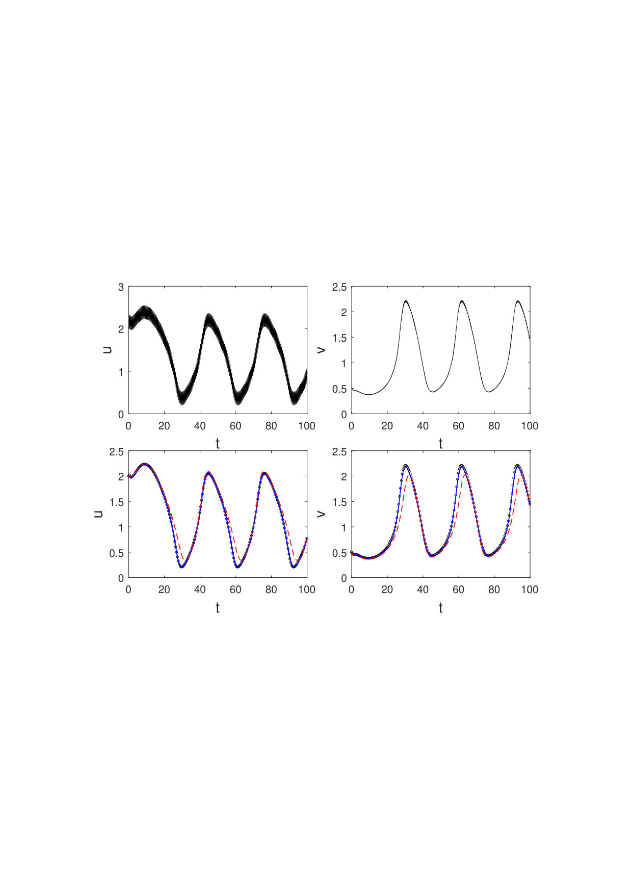 Figure 4
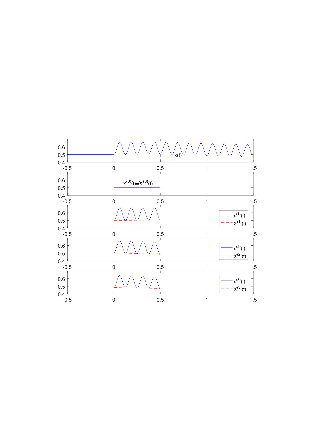 Figure 2
| AS2 | 3.31(-4) | 8.83(-5) | 2.28(-5) | 5.77(-6) | 1.46(-6) | 3.66(-7) |
|---|---|---|---|---|---|---|
| AS3 | 1.04(-4) | 1.28(-5) | 1.59(-6) | 1.96(-7) | 2.07(-8) | 2.30(-9) |
Peer Reviews
No public reviews on file for this paper yet. If you reviewed it on a platform where reviews are public (OpenReview, ICLR, NeurIPS, ICML), you can paste yours below so the community can read it here.
Videos
No videos yet. Explain this paper in a talk, walkthrough, or lecture? Add one.
Taxonomy
TopicsNonlinear Dynamics and Pattern Formation · Numerical methods for differential equations · Stability and Controllability of Differential Equations
Word-series high-order averaging of highly oscillatory differential equations with delay
J. M. Sanz-Serna
Departamento de Matemáticas, Universidad Carlos III de Madrid
Avenida de la Universidad 30, E-28911 Leganés (Madrid), Spain
Email: [email protected]
Beibei Zhu
National Center for Mathematics and Interdisciplinary Science
Academy of Mathematics and Systems Science
Chinese Academy of Sciences, Beijing 100190, P.R. China
Email: [email protected]
Abstract
We show that, for appropriate combinations of the values of the delay and the forcing frequency, it is possible to obtain easily high-order averaged versions of periodically forced systems of delay differential equations with constant delay. Our approach is based on the use of word-series techniques to obtain high-order averaged equations for differential equations without delay.
Mathematical Subject Classification (2010) 34C29
Keywords Delay differential equations, stroboscopic averaging, word series
1 Introduction
We show that, for appropriate combinations of the values of the delay and the forcing frequency, it is possible to obtain easily high-order averaged systems of periodically forced systems of delay differential equations with constant delay.
The well-known theory of averaging [20, 14] studies the reduction, by means of time-dependent changes of variables, of (nonautonomous) forced systems of differential equations to autonomous time-independent systems (averaged systems). Such a reduction is useful because autonomous systems are easier to analyze than their nonautonomous counterparts. In addition, the numerical integration of periodically or quasi-periodically forced systems may be expensive because typically integrators have to operate with step-sizes that are small with respect to the shortest period present in the forcing; in those cases, integrating an averaged version of the given system may be very advantageous.
In many occasions averaging is only carried out to first order. When the forcing is periodic this simply means replacing the right-hand side of the given oscillatory differential system by its average over one period of the forcing. In other cases, first order averaging is not enough and it is desirable to obtain averaged systems that provide more accurate approximations. For ordinary differential equations without delay the obtention of high-order averaging may be a daunting task, even with the help of a symbolic manipulator. The series of papers [6, 7, 8, 9, 15, 10, 18, 19] has developed a technique that, in the absence of delays, makes it possible to compute high-order averaged systems through simple recursions. The technique is based on the theory of word series [16], formal series [21] that have numerous applications in the fields of deterministic or stochastic dynamical systems [17] and numerical integration [1, 2].
The difficulties in obtaining high-order averaged systems are compounded if the system to be averaged has delays. In this paper we show that, for periodically forced differential systems with constant delay, it is possible to obtain high-order averaged systems by an application of the word-series results in [6, 7, 8, 9, 15, 10, 18, 19]. The simple treatment presented here is only possible when the forcing period is a submultiple of the delay, a hypothesis whose scope is discussed in Section 3.
Section 2 recalls the word-series averaging of systems of differential equations without delay. Section 3 contains the main idea and Section 4 describes an application that shows how third-order averaging succeeds where second-order averaging fails. The final Section 5 concludes.
2 Preliminaries
In this section we summarize the word-series averaging of differential equations without delay [18]. This summary will provide the foundation to address later the case with delay.
Let us consider highly oscillatory initial value problems of the form
[TABLE]
Here the smooth function is -periodic in its second argument , with Fourier expansion
[TABLE]
and the parameter is the angular frequency of the fast periodic forcing. The corresponding period is .
In the theory of word series the set of indices in (2) is seen as an (infinite) alphabet and for , the elements of are regarded as words consisting of letters of this alphabet. There is also an empty word with letters. Given (1), to each word one associates the corresponding word basis function , a map . By definition, for words with one letter , the word basis function is the Fourier coefficient in (2). For words with letters, we define recursively
[TABLE]
where is the Jacobian matrix of . For the empty word , the basis function is the identity map .
The set of all words (including the empty word) is denoted by and refers to the set of all mappings . For and , denotes the value of at . To each we associate the corresponding word series (relative to the mappings in (2)); this is the formal series
[TABLE]
whose terms are maps . The complex numbers are the coefficients of the series. As an example consider the case where and for each nonempty word ; in this case .
As proved in [7, 18] (see [19] for an alternative technique), there exist and a -periodic map such that the solution of (1) may be written as
[TABLE]
where is the solution of
[TABLE]
In this way, the time-dependent change of variables in (4) transforms the given highly oscillatory initial value problem into the initial value problem (5) where there is no periodic forcing. Therefore (5) provides an averaged version of (1). In addition, the coefficients are such that, at , , we have and for each nonempty word . This implies that, for those values of , the transformation is the identity map and it then follows that, in (4), at the strobocopic times, We then say that the change of variables is stroboscopic and that (5) is obtained from (1) through stroboscopic averaging. There are of course alternative forms of averaging; for instance one may impose the condition that the periodic change of variables has 0 average over one period, rather than being the identity at .
It is in order to point out that and depend on , but are otherwise universal in the sense that they do not change with the dimension or with the choice of . Such a universality implies that they may be computed once and for all; averaging a new differential system requires the computation of new basis functions but not of new coeffcients. The values and for may be computed easily by recursion with respect to the number of letters in the word ; the reader is referred to [7, 10, 18] for details.
In general, the formal series in the averaged system (5) and the formal series in the change of variables (4) do not converge and have to be truncated and of course the truncation introduces an error, see [8, 9]. For our purposes here we just mention that, if is truncated by eliminating all the terms in the series that correspond to words with more than letters, one obtains an initial value problem whose solution coincides at stroboscopic times with the solution except for an error of size as .111To approximate at times that are not stroboscopic one needs to apply to the solution of the truncated averaged system a change of variables obtained by truncating the series in (4) . The truncated averaged system with first order errors obtained by discarding contributions corresponding to words with two or more letters is found to be:
[TABLE]
as it may have been expected.
The truncated averaged system with second order errors is given by [7, 10, 18]
[TABLE]
Note that, is by definition the word-basis function associated with the one-letter words [math]. Furthermore, according to (3), the function is the word basis function associated to the word and similarly , are associated to and . Thus the right-hand side of (7) is indeed a word series (whose coefficients vanish for all words with 3 or more letters).
The closed form expression for the third order averaged system for the problem (1) with general may be seen in [7, 10, 18]. For order it is not practical to find the general expression of the averaged system and then to apply it to the specific instance of (1) at hand. One should rather find recursively the word basis functions corresponding to the of interest, perhaps with the help of a symbolic manipulator, see [15, 19] for additional details.
3 Highly oscillatory problems with delay
We now consider the -dimensional system with constant delay
[TABLE]
where is -periodic in its third argument, with Fourier expansion
[TABLE]
and is the angular frequency as above. Without loss of generality [22], it is assumed that the known function that specifies the initial history is independent of . Reference [22] contains a list of references to problems of this form that appear in different applications.
The developments that follow are based on the standing hypothesis that the delay is an integer multiple of the period , or in other words that is a stroboscopic time. Let us discuss this hypothesis. In some applications, the value of is given and the interest is in studying the behaviour of the solution of (8)–(9) for large , but there is some freedom as to the choice of the specific value of . In those cases, the theory below applies by choosing in such a way that is an integer. Similarly, our theory applies to situations where the interest is in a given, large value of and there is some freedom in the choice of to be used in the model. On the other hand, if the values of and are fixed, the material in this paper does not apply. In those cases finding high-order averaged systems may be extremely complicated (see e.g. the computations in [22]).
3.1 The averaging procedure
Assume that (8)–(9) is to be studied in a bounded interval of the form for a suitable integer . (This hypothesis is made at this stage for mathematical convenience to avoid systems of infinitely many differential equations; the averaged systems that we will find will be valid for all .) We introduce the functions (see Fig. 1).
[TABLE]
and note that determining these functions is clearly equivalent to determining the solution of (8)–(9) in the interval . The with satisfy the conditions
[TABLE]
and the differential equations
[TABLE]
Even though the relations (13) may be reminiscent of a two-point boundary value problem, we are facing here an initial value problem: is determined by solving the differential equation with with initial condition , once is known, is determined by solving the differential equation with with initial condition , etc.
By taking into account the periodicity of as a function of and our standing hypothesis that is a multiple of the period, the last display may be written as
[TABLE]
Note that this would be a system of the form (1) for the -dimensional vector if it were not for the fact that the right-hand side of the equation corresponding to contains , a known function of given in (11). In order to have a system of the form (1), where the right-hand side only depends on through the combination , we proceed as follows. We introduce the -dimensional vector of unknown functions of the variable
[TABLE]
and add to (14) the differential equations
[TABLE]
(the dot represents differentiation) subject to the initial conditions
[TABLE]
The solution of the initial value problem (15)–(16) is obviously and . Now (15) in tandem with (14) is a -dimensional system of the form (1) that may be stroboscopically averaged by following the procedure described in the previous section. If is the averaged counterpart of , we are interested in the solutions of the averaged system that satisfy (cf. (13))
[TABLE]
so that it is possible to define a continuous function in the interval by patching together the different ,
[TABLE]
thus undoing the process that we used to move from the solution of (8)–(9) to the functions in (11)–(12), see Fig. 1. In this way the averaged delay equation is obtained by patching the equations for the . The whole procedure will be clear after we present the simple case of the first-order averaged system.
3.2 The first-order averaged system
If denotes the right-hand side of the oscillatory system of differential equations (14)–(15) satisfied by , the Fourier series for (cf. (2)) has coefficients
[TABLE]
where the are the Fourier coefficients of as in (10). According to (6), the first-order averaged system of differential equation without delay in the interval is therefore given by (capital letters denote averaged dependent variables)
[TABLE]
This system is to be solved with the conditions , and (17). Clearly , and therefore the function in (18) satisfies the averaged delay problem (cf. (8)–(9))
[TABLE]
as one could have easily guessed. Note that does not feature in the averaged problem, as we pointed out above.
The solutions and of (8)–(9) and (19)–(20) differ at stroboscopic times by as we prove next. That at stroboscopic times follows by considering that, for those values of , , and because of the properties of stroboscopic averaging of ordinary differential equations without delay. For stroboscopic times in the interval the situation is slightly more complicated because in addition to the error arising from truncating (5) there is an additional source of error: in this interval , but and do not share the same initial value at . However the difference of initial values is , which we know is of size . It follows that also at stroboscopic times . The iteration of this argument leads to the conclusion we seek, i.e. whenever is a stroboscopic time. Of course the constant implied in the notation of course depends on (and in general will grow as increases).
3.3 Second-order averaged system
If rather than using the truncated averaged system (6), we use (7), the procedure described above leads, after some simple algebra, to an averaged problem given by (20) and a delay differential equation of the form
[TABLE]
with
[TABLE]
and
[TABLE]
valid for . In these expressions and denote the Jacobian matrices of with respect to and respectively. By arguing as in the first order case, one proves that at stroboscopic times the difference between the solution of (8)–(9) the solution of (20)–(22) is .
3.4 Third- and higher order averaged systems
It is still feasible to obtain in closed form the third-order averaged system for delay problems starting from the corresponding expression for the case without delay given in [7, 10, 18]. The expression of the averaged delay system one obtains in this way is lengthy and will not be reproduced here. In fact for order 3 or higher, the best approach is to find recursively the word basis functions for the system (14)–(15) for the specific of interest.
For an averaged system of order , the right-hand side of the system has expressions corresponding to the intervals , …, , and . (Recall that the second-order averaged system displayed above has two expressions.)
4 An example
As an illustration, we consider the system
[TABLE]
where and are parameters. There are two periodic forcing terms; the forcing is slow (i.e. the frequency is of moderate size) and , , is fast. When there is no forcing (), the system represents a delayed genetic toggle switch, a synthetic gene regulatory network [12]. The forced system was studied in [11] as an instance of the emergence of vibrational resonance [13, 15], i.e. the enhancement, due to the presence of the fast forcing, of the response of the system to the slow forcing.
In order to have a system of the form (8) it is necessary to rewrite as , where is a new dependent variable defined by the differential equation and the initial condition at (this is of course the technique used above in (15)–(16) to deal with the slow dependence on of the right-hand side of (14)). Thus only the fast forcing is averaged. After computing recursively the required word basis functions and coefficients, the third-order averaged system is found to be given by
[TABLE]
for , and
[TABLE]
for . (As pointed out above, in general, the third-order averaged system has an analytic expression in and a different analytic expression in ; for the problem at hand those two expressions happen to coincide.) The second-order averaged system may be retrieved from the last displays by omitting the terms that have an factor in the denominator.
We have integrated numerically the true dynamics and the second- and third-order averaged systems. The integrations were carried out with the Matlab function dde23 with relative and absolute tolerances and respectively. For the choice , , , , , and , with constant history , , (an equilibrium of the unforced system), Table 1 presents the maximum error in at stroboscopic times in the short interval ; in agreement with the theory, the error behavior is for second-order averaging and for third-order averaging.
In Fig. 2, the parameters are , , , , , and , with constant history , , (again an equilibrium of the unforced system). The integration is perfomed in the interval . The numerical integration of the oscillatory problem needed 261.0 seconds, a quantity that has to be compared with the 2.1 and 2.6 seconds required to integrate the second- and third-order averaged systems respectively. In studies like those performed in [11], where the oscillatory systems has to be integrated in long time intervals for many different choices of the values of the parameters, the advantage of averaging is then clear.
5 Conclusion
We have showed that, when the delay is a multiple of the forcing period, it is possible to extend to periodically forced, constant delay problems, the word-series approach to the systematic derivation of high-order averaged systems. We have presented an example where the new technique has been applied to a system of interest in connection with the phenomenon of vibrational resonance.
To conclude let us point out that, for ordinary differential equations, it is possible to compute numerically a stroboscopically averaged solution without the explicit knowledge of the corresponding averaged system; the information on the averaged system required by the integrator is derived by numerically simulating the oscillatory system (1) [3, 4]. Such techniques have been extended to delay differential equations [22, 5].
Acknowledgements. J.M.S. was supported by project MTM2016-77660-P(AEI/ FEDER, UE) funded by MINECO (Spain). B. Z. is supported by the National Natural Science Foundation of China (Grant No. 11771438) and the Postdoctoral Fund Project of China (Grant No. 2018M641506) and in addition by the National Center for Mathematics and Interdisciplinary Sciences, CAS.
The reference list from the paper itself. Each links out to its DOI / PubMed record.
- 1[1] Alamo, A., Sanz-Serna, J.M., (2016), A technique for studying strong and weak local errors of splitting stochastic integrators. SIAM J. Numer. Anal. 54 , 3239–3257.
- 2[2] Alamo, A., Sanz-Serna, J.M., (2019), Word combinatorics for stochastic differential equations: splitting integrators, Comm. on Pure Applied Anal. 18 , 2163-2195.
- 3Calvo et al. [2011 a] Calvo, M.P., Chartier, Ph., Murua A., and Sanz-Serna, J.M., (2011 a), Numerical stroboscopic averaging for OD Es and DA Es. Appl. Numer. Math. 61 , 1077–1095.
- 4Calvo et al. [2011 b] Calvo, M.P., Chartier, Ph., Murua, A., and Sanz-Serna, J.M., (2011 b) A stroboscopic method for highly oscillatory problems. In: B. Engquist, O. Runborg and R. Tsai (eds.) Numerical Analysis and Multiscale Computations, pp. 73–87. Springer, New York.
- 5[5] Calvo, M.P., Zhu, B., and Sanz-Serna J.M., (2019), High-order stroboscopic averaging methods for highly oscillatory delay problems, submitted.
- 6[6] Chartier, Ph., Murua, A., and Sanz-Serna, J.M., (2010), Higher-order averaging, formal series and numerical integration I: B-series, Found. Comput. Math. 10 , 695-727.
- 7[7] Chartier, Ph., Murua, A., and Sanz-Serna, J.M., (2012 a), Higher-order averaging, formal series and numerical integration II: the quasi-periodic case. Found. Comput. Maths. 12 , 471-508.
- 8[8] Chartier, Ph., Murua, A., and Sanz-Serna, J.M., (2012 b), A formal series approach to averaging: exponentially small error estimates. DCDS A 32 , 3009-3027.