Optimal placement of inertia and primary control : a matrix perturbation theory approach
Laurent Pagnier, Philippe Jacquod

TL;DR
This paper introduces a matrix perturbation theory approach to optimize the placement of inertia and primary control in power grids with heterogeneous parameters, improving stability and disturbance mitigation.
Contribution
It develops analytical tools and algorithms for optimal placement of inertia and primary control considering heterogeneity, advancing beyond previous uniform assumptions.
Findings
Optimal inertia distribution is geographically homogeneous.
Primary control should be placed on slow network modes.
Algorithms effectively determine optimal control placement.
Abstract
The increasing penetration of inertialess new renewable energy sources reduces the overall mechanical inertia available in power grids and accordingly raises a number of issues of grid stability over short to medium time scales. It has been suggested that this reduction of overall inertia can be compensated to some extent by the deployment of substitution inertia - synthetic inertia, flywheels or synchronous condensers. Of particular importance is to optimize the placement of the limited available substitution inertia, to mitigate voltage angle and frequency disturbances following a fault such as an abrupt power loss. Performance measures in the form of H2-norms have been recently introduced to evaluate the overall magnitude of such disturbances on an electric power grid. However, despite the mathematical conveniance of these measures, analytical results can be obtained only under…
Click any figure to enlarge with its caption.
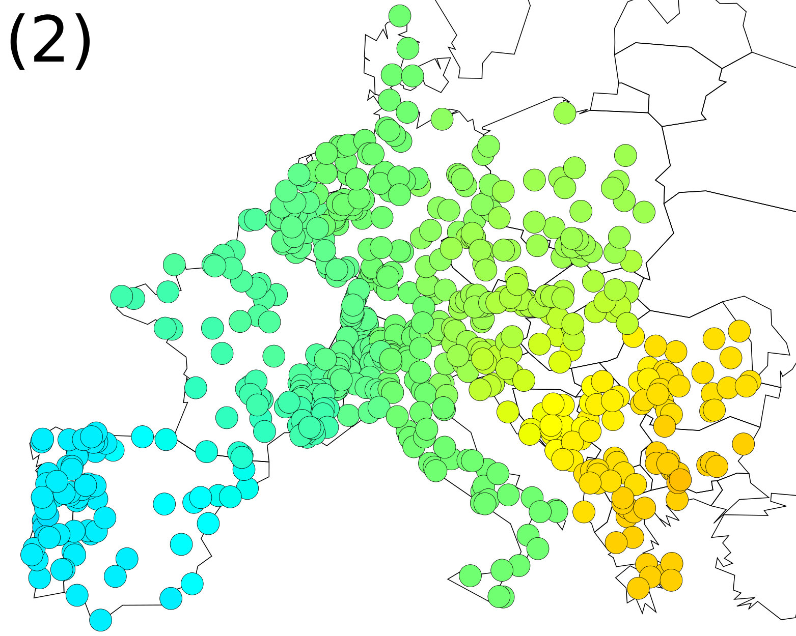 Figure 1
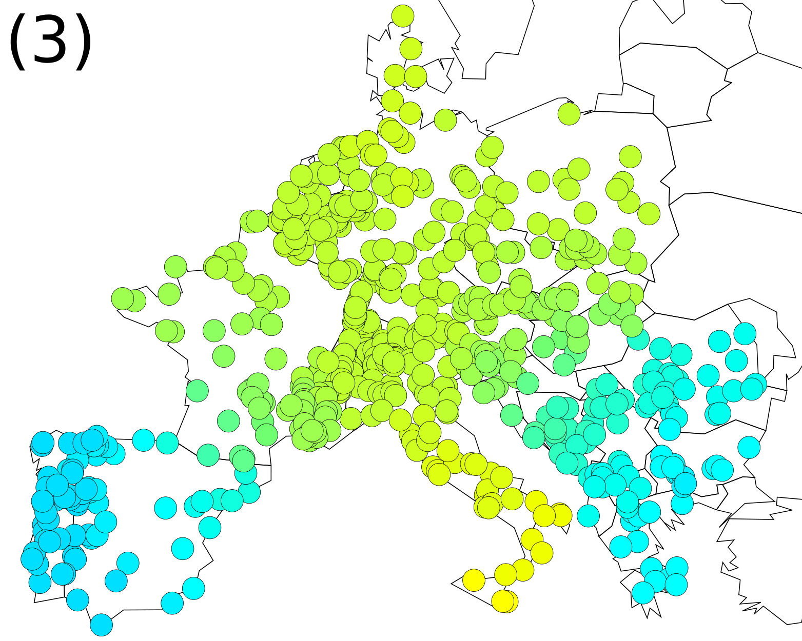 Figure 2
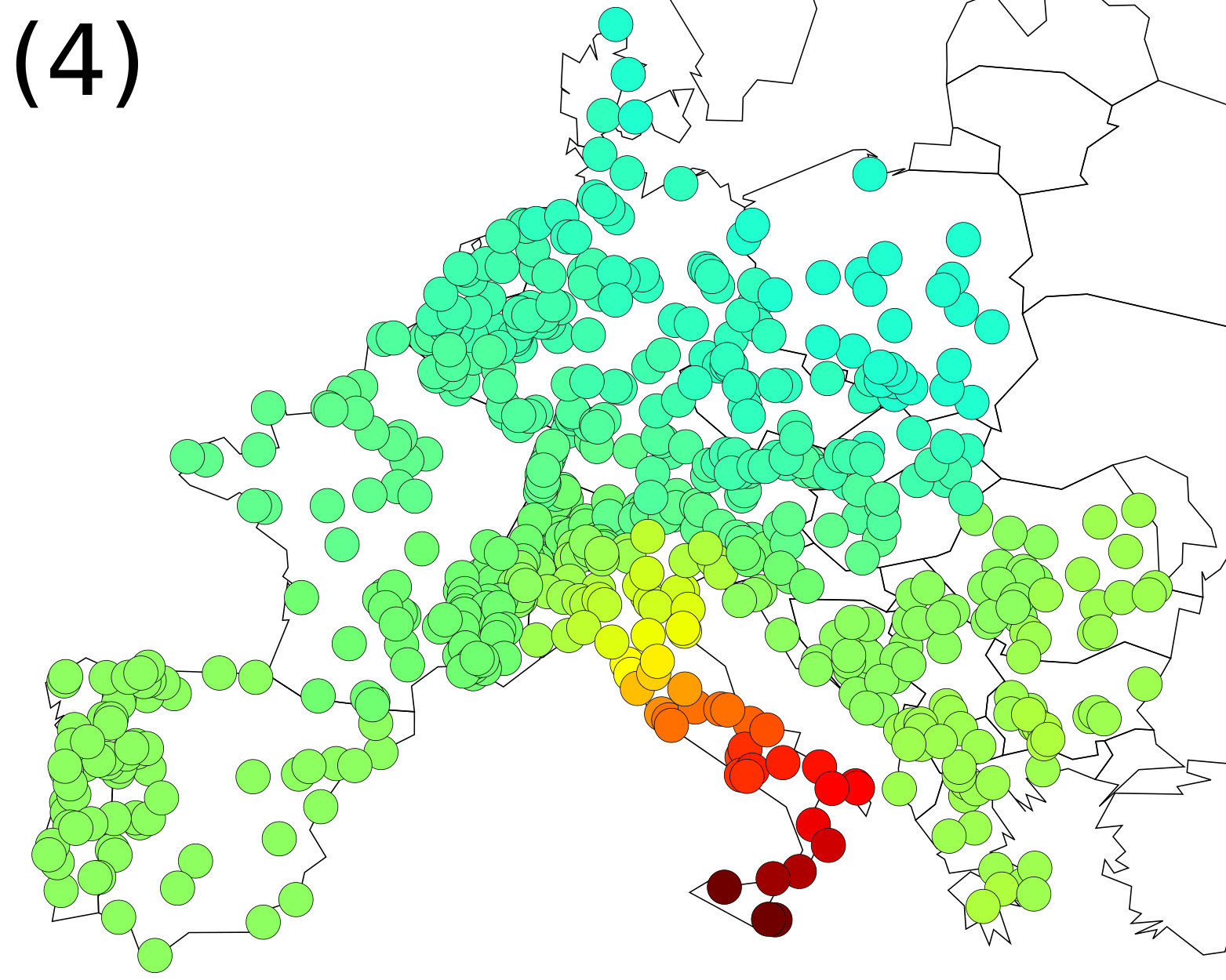 Figure 3
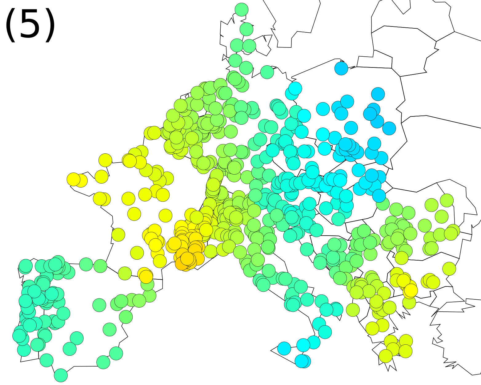 Figure 4
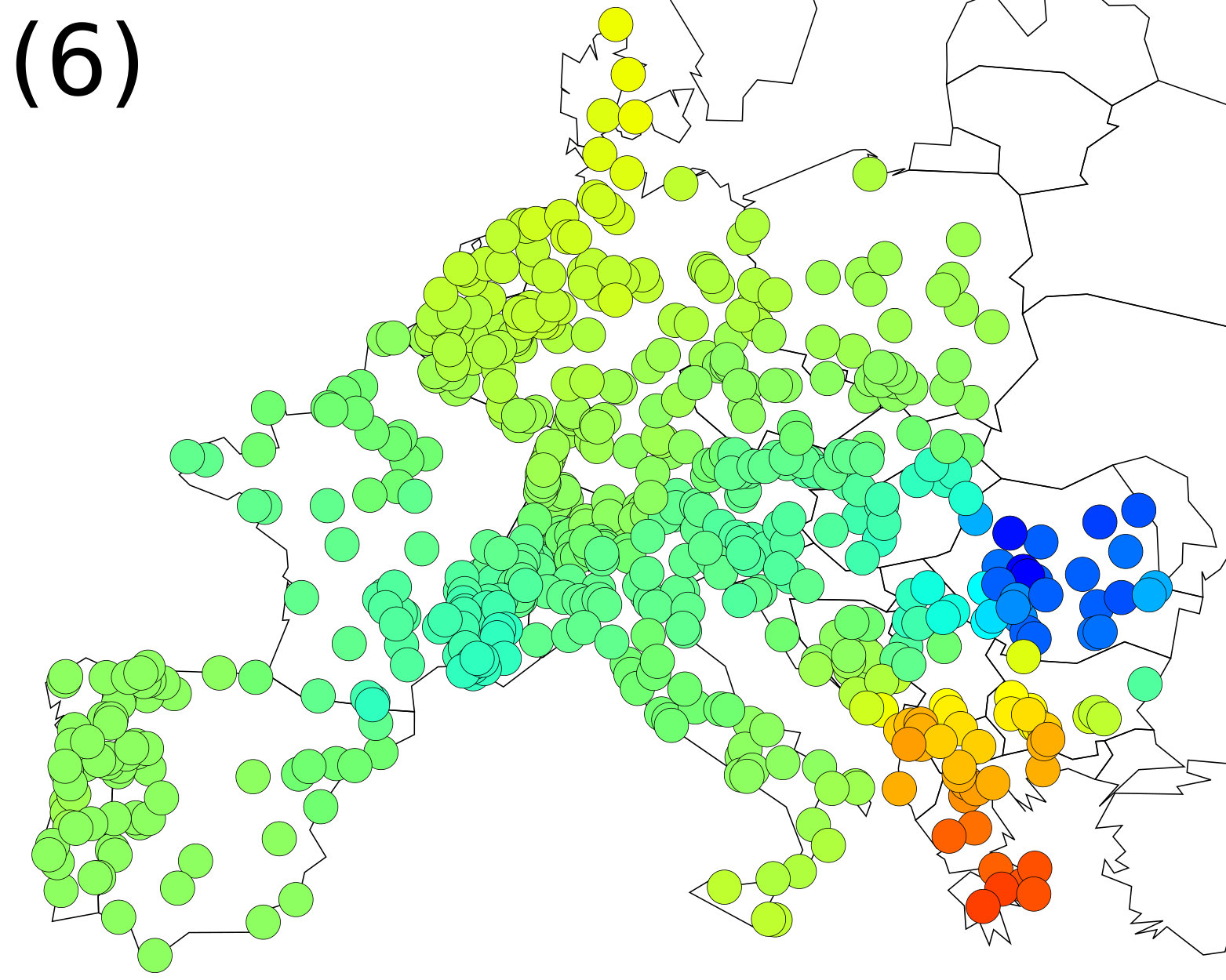 Figure 5
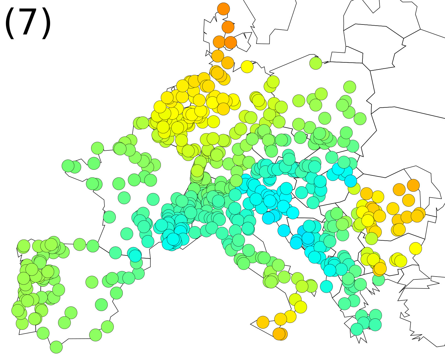 Figure 6
 Figure 7
 Figure 8
 Figure 9
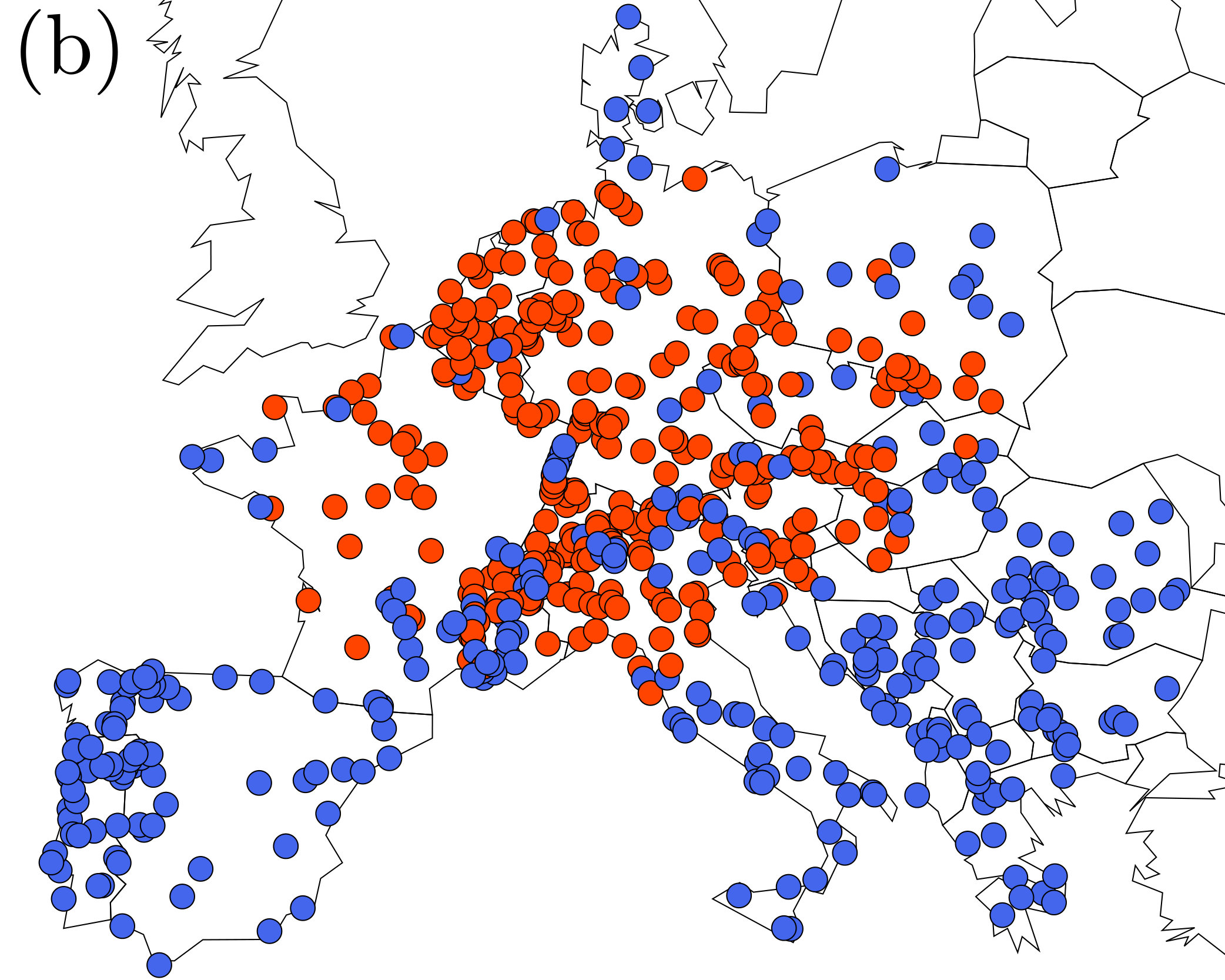 Figure 10
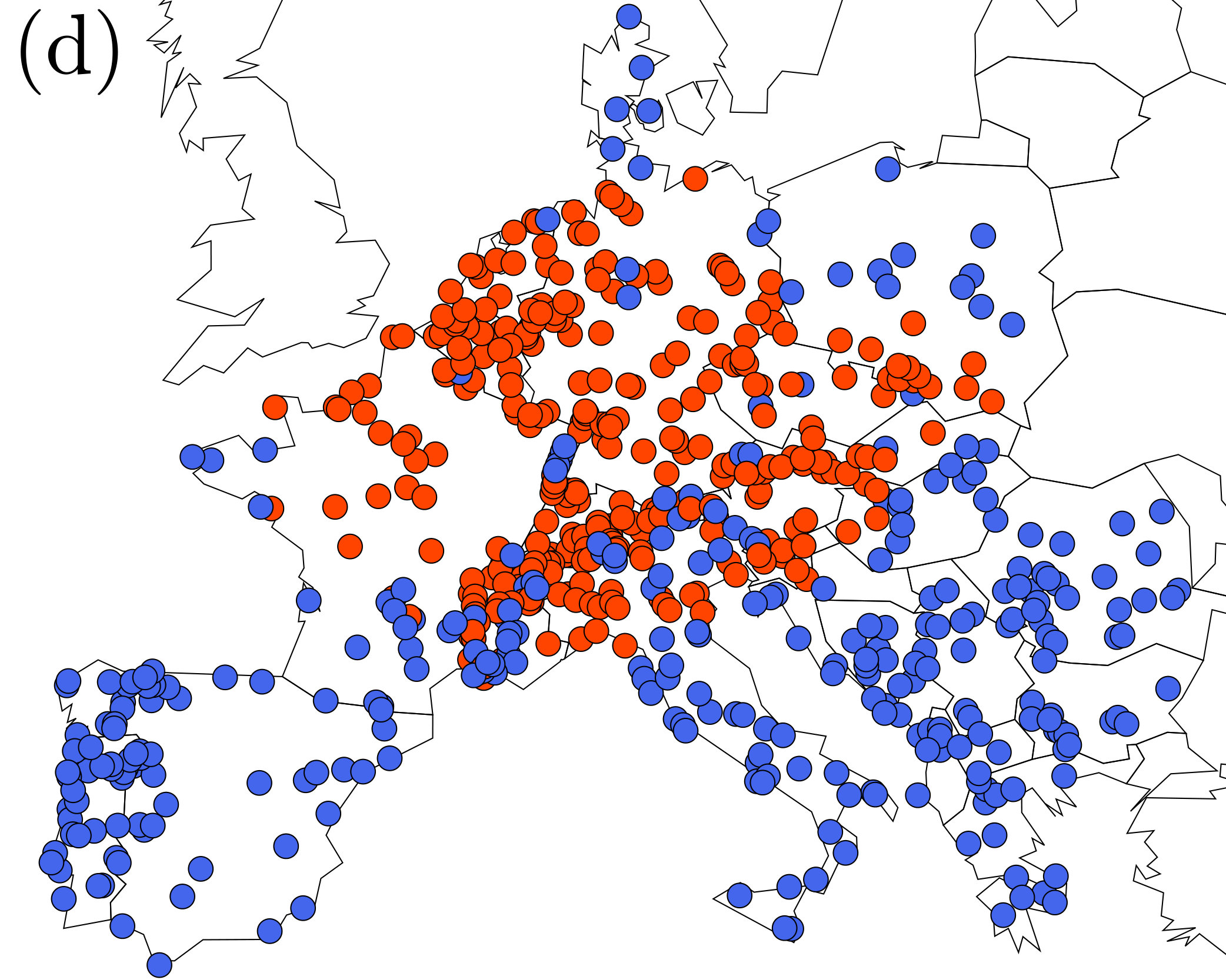 Figure 11
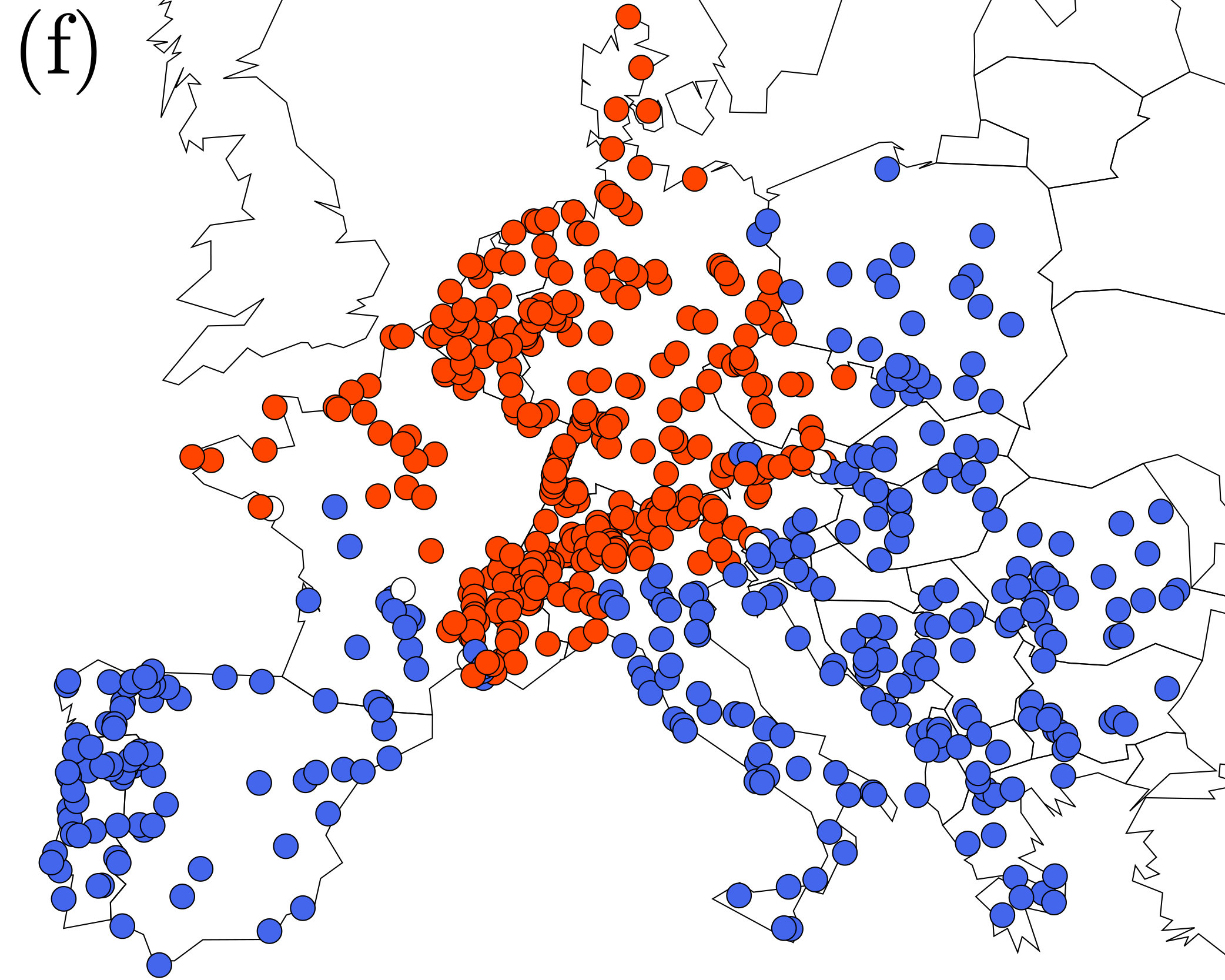 Figure 12
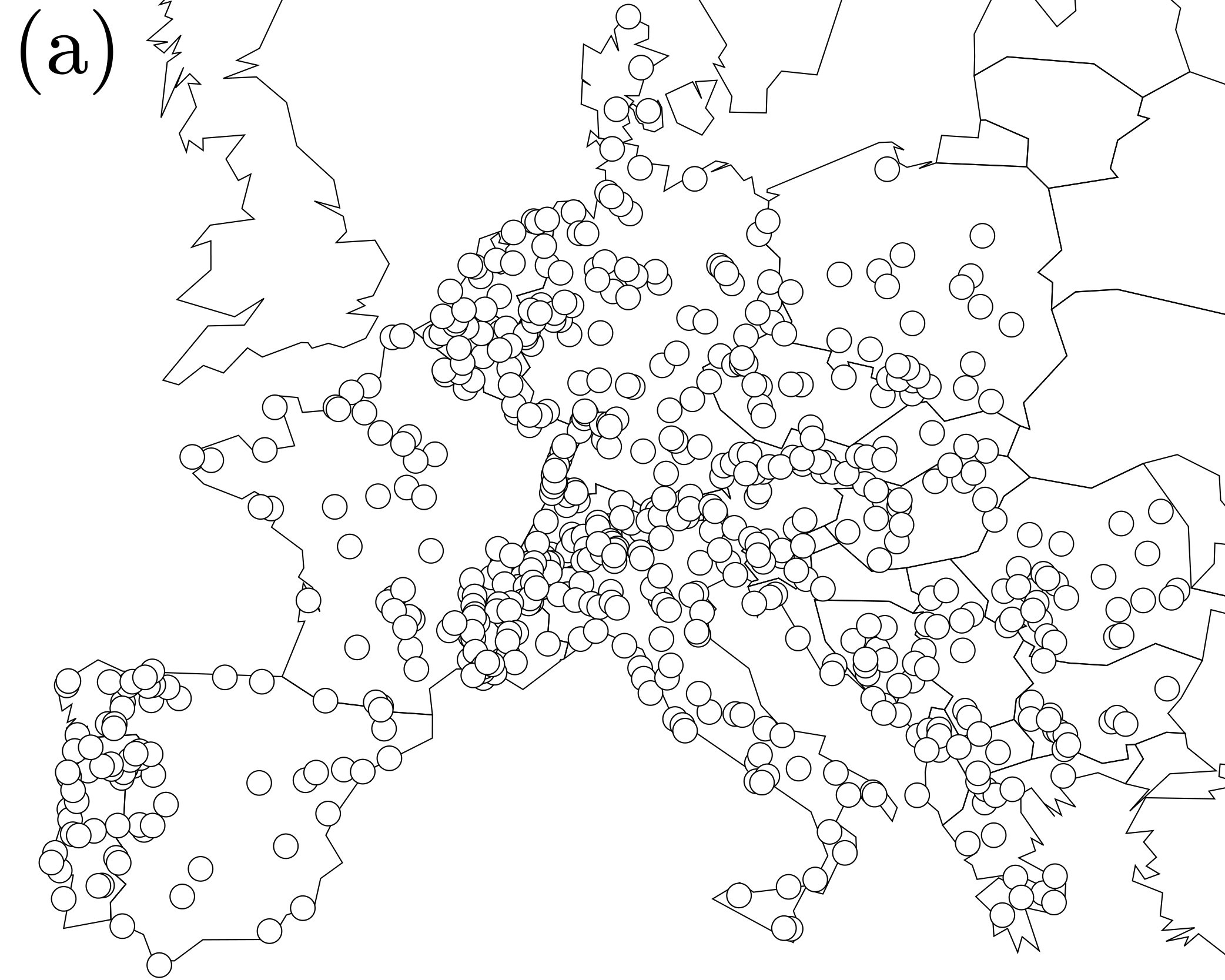 Figure 13
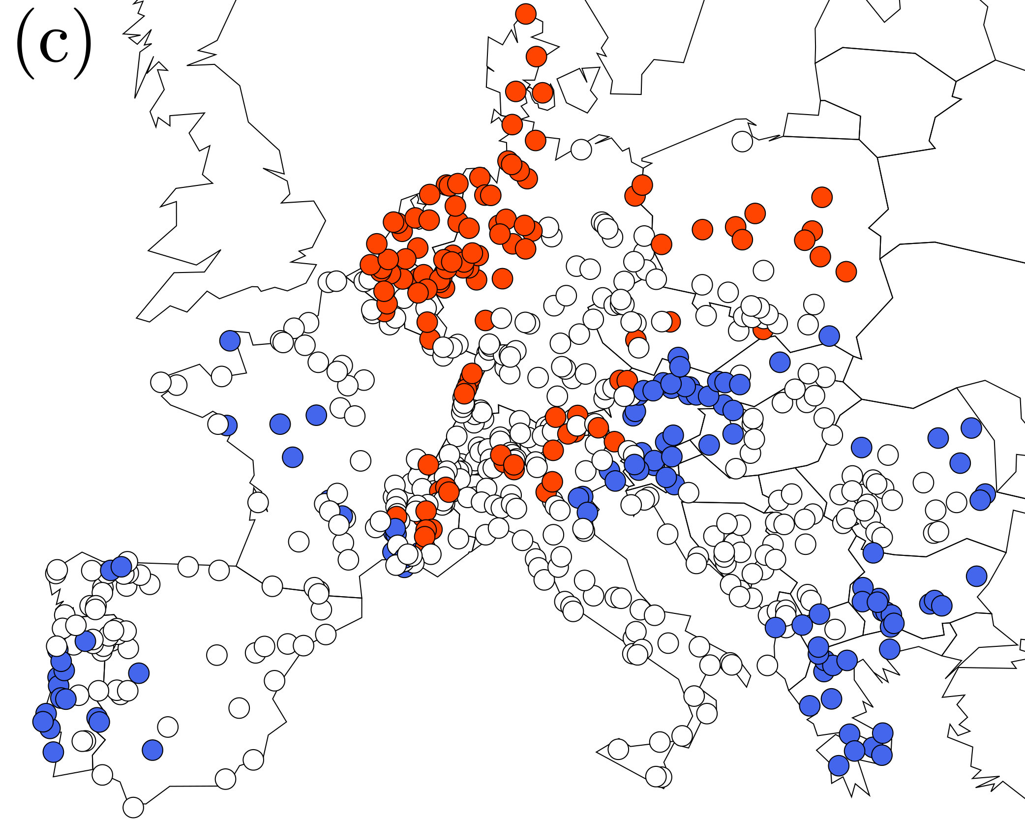 Figure 14
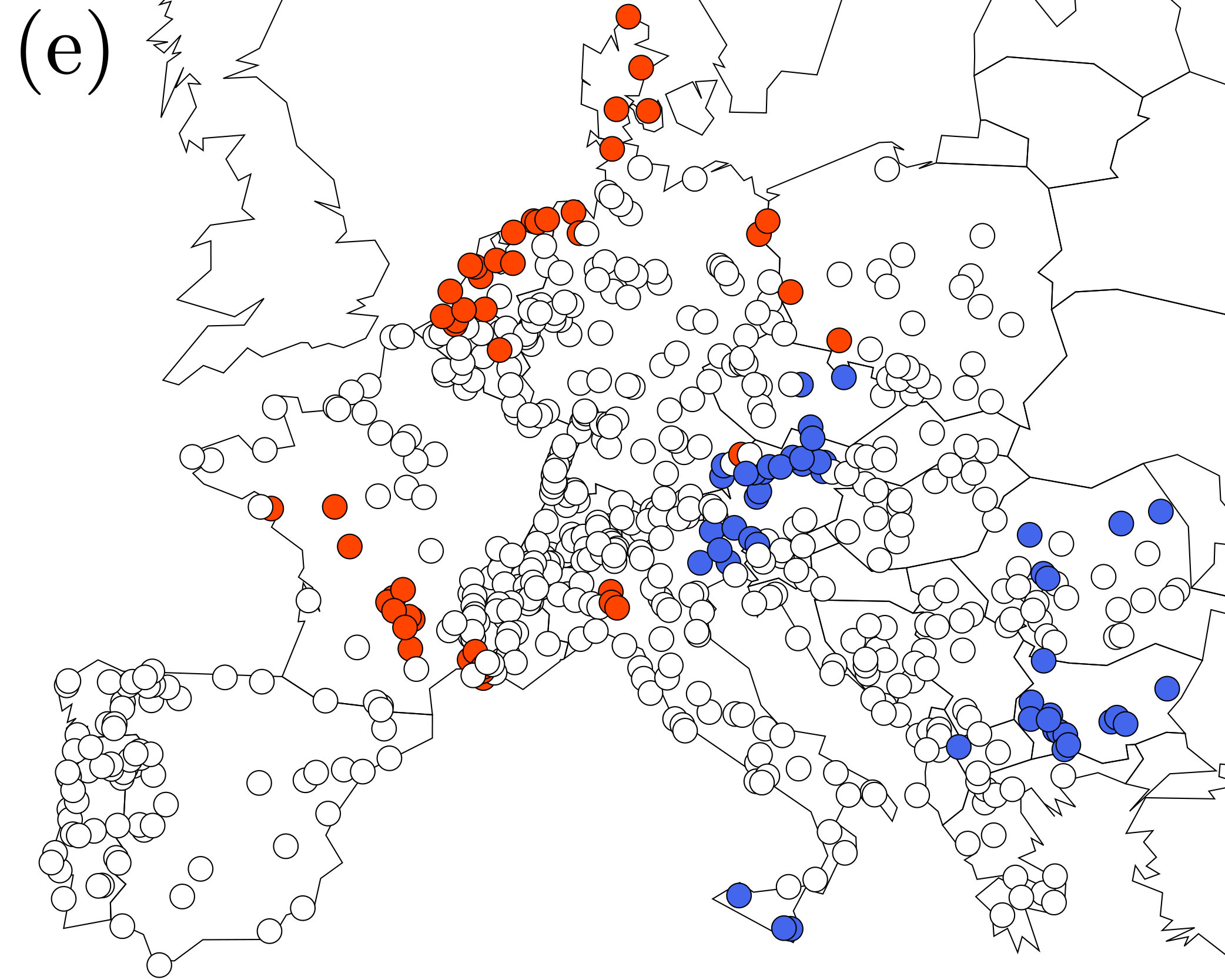 Figure 15
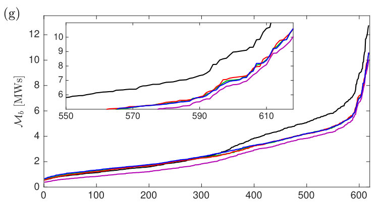 Figure 16
Peer Reviews
No public reviews on file for this paper yet. If you reviewed it on a platform where reviews are public (OpenReview, ICLR, NeurIPS, ICML), you can paste yours below so the community can read it here.
Videos
No videos yet. Explain this paper in a talk, walkthrough, or lecture? Add one.
Optimal placement of inertia and primary control : a matrix perturbation theory approach
Laurent Pagnier, and Philippe Jacquod
Abstract
The increasing penetration of inertialess new renewable energy sources reduces the overall mechanical inertia available in power grids and accordingly raises a number of issues of grid stability over short to medium time scales. It has been suggested that this reduction of overall inertia can be compensated to some extent by the deployment of substitution inertia - synthetic inertia, flywheels or synchronous condensers. Of particular importance is to optimize the placement of the limited available substitution inertia, to mitigate voltage angle and frequency disturbances following a fault such as an abrupt power loss. Performance measures in the form of norms have been recently introduced to evaluate the overall magnitude of such disturbances on an electric power grid. However, despite the mathematical conveniance of these measures, analytical results can be obtained only under rather restrictive assumptions of uniform damping ratio, or homogeneous distribution of inertia and/or primary control in the system. Here, we introduce matrix perturbation theory to obtain analytical results for optimal inertia and primary control placement where both are heterogeneous. Armed with that efficient tool, we construct two simple algorithms that independently determine the optimal geographical distribution of inertia and primary control. These algorithms are then implemented on a model of the synchronous transmission grid of continental Europe. We find that the optimal distribution of inertia is geographically homogeneous but that primary control should be mainly located on the slow modes of the network, where the intrinsic grid dynamics takes more time to damp frequency disturbances.
I Introduction
The penetration of new renewable energy sources (RES) such as photovoltaic panels and wind turbines is increasing in most electric power grids worldwide. In their current configuration, these energy sources are essentially inertialess, and their increased penetration leads to low inertia situations in periods of high RES production [1]. This raises important issues of power grid stability, which is of higher concern to transmission system operators than the volatility of the RES productions [2, 3]. The substitution of traditional productions based on synchronous machines with inertialess RES may in particular lead to geographically inhomogeneous inertia profiles. It has been suggested to deploy substitution inertia – synthetic inertia, flywheels or synchronous condensers – to compensate locally or globally for missing inertia. Two related question naturally arise, which are (i) where is it safe to substitute synchronous machines with inertialess RES and (ii) where is it optimal to distribute substitution inertia ? Problem (ii) has been investigated in small power grid models with up to a dozen buses, optimizing the geographical distribution of inertia against cost functions based on eigenvalue damping ratios [4], -norms [5, 6] or RoCoF [7, 8] and frequency excursions [8]. Investigations of problem (i) on large power grids emphasized the importance of the geographical extent of the slow network modes [9]. Numerical optimization can certainly be performed for any given network on a case-by-case basis, however it is highly desirable to shed light on the problem with analytical results. So far, such results have been either restricted to small systems or derived under the assumption that damping and inertia parameters, or their ratio, are homogeneous. In this manuscript we go beyond these assumptions and construct an approach applicable to large power grids with inhomogeneous independent damping and inertia parameters.
Inspired by theoretical physics, we introduce matrix perturbation theory [10] as an analytical tool to tackle this problem. That method is widely used in quantum physics, where it delivers approximate solutions to complex, perturbed problems, extrapolated from known, exact solutions of integrable problems [11]. The approximation is valid as long as the difference between the two problems is small and it makes sense to consider the full, complex problem as a perturbation of the exactly soluble, simpler problem. The procedure is spectral in nature. It identifies a small, dimensionless parameter in which eigenvalues and eigenvectors of the perturbed problem can be systematically expanded in a series not unlike a Taylor-expansion about the unperturbed, integrable solution. Depending on the value of that small parameter, the series can be truncated at low orders already and still deliver rather accurate results. In the context of electric power grids, the method was applied for instance in Ref. [12], where quadratic performance measures similar to those discussed below were calculated following a line fault, starting from the eigenvalues and eigenvectors of the network Laplacian before the fault.
In this paper, we apply matrix perturbation theory [10] to calculate performance measures following an abrupt power loss in the case of a transmission power grid with geographically inhomogeneous inertia and damping (primary control) parameters. Our perturbation theory is an expansion in two parameters which are the maximal deviations and of the rotational inertia and damping parameters from their average values and . The approach is valid as long as these local deviations are small, , . These conditions tolerate in principle that inertia and damping parameters vanish or are twice as large as their average on some buses. The main step forward brought about by our approach is that we are able to derive analytical results without relying on the often used homogeneity assumptions that damping, inertia or their ratio is constant - assumptions which are not satisfied in real electric power grids. Our main results are given in Theorems 1 and 2 below, which formulate algorithms for optimal placement of local inertia and damping parameters. The spectral decomposition approach used here has recently drawn the attention of a number of groups and has been used to calculate performance measures in power grids and consensus algorithms e.g. in [7, 13, 14, 15].
The article is organized as follows. Section II deals with the case where inertia and primary control are uniformly distributed in the system. The performance measure that quantifies system disturbances is introduced and we calculate its value for abrupt power losses. In Section III we apply matrix perturbation theory to calculate the sensitivities of our measure in local variations of inertia and primary control. Section IV presents the optional placement of inertia and primary control in the case of weak inhomogeneity. In Section V we apply our optimal placements to the continental European grid. Section VI concludes our article.
II Homogeneous case
We are interested in the dynamical response of an electric power grid to a disturbance such as an abrupt power loss. To that end, we consider the power system dynamics in the lossless line approximation, which is a standard approximation used for high voltage transmission grids [16]. That dynamics is governed by the swing equations,
[TABLE]
which determine the time-evolution of the voltage angles and frequencies at each of the buses labelled in the power grid in a rotating frame such that measures the angle frequency deviation to the rated grid frequency of 50 or 60 Hz. Each bus is characterized by inertia, , and damping, , parameters and is the active power injected () or extracted () at bus . We introduce the damping ratio . Buses are connected to one another via lines with susceptances . Stationary solutions are power flow solutions determined by . Under a change in active power , linearizing the dynamics about such a solution with gives, in matrix form,
[TABLE]
where , and voltage angles and frequencies are cast into vectors and . The Laplacian matrix has matrix elements , for and .
II-A Exact solution for homogeneous damping ratio
When the damping ratio is constant, , , (2) can be integrated exactly [7, 12]. To see this we first transform angle coordinates as to obtain
[TABLE]
where we introduced the diagonal matrix . The inertia-weighted matrix is real and symmetric, therefore it can be diagonalized
[TABLE]
with an orthogonal matrix , the row of which gives the components , of the eigenvector of . The diagonal matrix contains the eigenvalues of with . For connected networks only the smallest eigenvalue vanishes, which follows from the zero row and column sum property of the Laplacian matrix . Rewriting (3) in the basis diagonalizing gives
[TABLE]
where . This change of coordinates is nothing but a spectral decomposition of angle deviations into their components in the basis of eigenvectors of . These components are cast in the vector . The formulation (5) of the problem makes it clearer that, if is a multiple of identity, the problem can be recast as a diagonal ordinary differential equation problem that can be exactly integrated. This is done below in (23), and provides an exact solution about which we will construct a matrix perturbation theory in the next sections.
Proposition 1** (Unperturbed evolution).**
For an abrupt power loss, , with the Heaviside step function defined by , , and with homogeneous damping ratio, with the identity matrix , the frequency coordinates evolve independently as
[TABLE]
where and .
This result generalizes Theorem III.3 of [14].
Proof:
The proof goes along the lines of the diagonalization procedure proposed in [7, 12, 17]. Equation (5) can be rewritten as
[TABLE]
where and is the matrix of zeroes. The matrix is block-diagonal up to a permutation of rows and columns [12], and can easily be diagonalized block by block, where each block corresponds to one of the eigenvalues of . The block is diagonalized by the transformation
[TABLE]
with the eigenvalues of the block,
[TABLE]
The two rows (columns) of () give the nonzero components of the two left (right) eigenvectors () of . Following this transformation, (7) reads
[TABLE]
The solutions of (23) are
[TABLE]
Inserting (24) back into (14), one finally finds (6) which proves the proposition. ∎
II-B Performance measure
We want to mitigate disturbances following an abrupt power loss. To that end, we use performance measures which evaluate the overall disturbance magnitude over time and the whole power grid. Performance measures have been proposed, which can be formulated as and squared norms of linear systems [6, 7, 12, 17, 18, 19, 20, 21, 22, 23] and are time-integrated quadratic forms in the angle, , or frequency, , deviations. Here we focus on frequency deviations and use the following performance measure
[TABLE]
where is the instantaneous average frequency vector with components
[TABLE]
It is straightforward to see that reads
[TABLE]
when rewritten in the eigenbasis of , once one notices that the first eigenvector of (the one with zero eigenvalue) has components .
Proposition 2**.**
For an abrupt power loss, on a single bus labeled , , and with an homogeneous damping ratio, with the identity matrix ,
[TABLE]
in terms of the eigenvalues and the components of the eigenvectors of .
Note that we introduced the subscript to indicate that the fault is localized on that bus only. The power loss is modeled as with with the Kronecker symbol if and 0 otherwise.
Proof:
Equation (6) straightforwardly gives
[TABLE]
which, when summed over gives (28). ∎
Remark 1**.**
For homogeneous inertia coefficients, , the eigenvectors and eigenvalues of the inertia-weighted Laplacian defined in (3) are given by , and , in terms of the eigenvectors and eigenvalues of the Laplacian . In that case, the performance measure reads
[TABLE]
where the superscript (0) refers to inertia homogeneity. This expression has an interesting graph theoretic interpreation. We recall the definitions of the resistance distance between two nodes on the network, the associated centrality and the generalized Kirchhoff indices [22, 24],
[TABLE]
where is the Moore–Penrose pseudo inverse of . With these definitions, one can show that [15, 22, 25]
[TABLE]
by using the spectral representation of the resistance distance [26, 27]
[TABLE]
Because is a global quantity characterizing the network, it follows from (30) with (34) that, when inertia and primary control are homogeneously distributed in the system, the disturbance magnitude as measured by is larger for disturbances on peripheral nodes [9, 28].
III Matrix perturbation
The previous section treats the case where inertia and primary control are uniformly distributed in the system. Our goal is to lift that restriction and to obtain when some mild inhomogeneities are present. We parametrize these inhomogeneities by writing
[TABLE]
with the average and and the maximum deviation amplitudes and of inertia and damping ratio. Inhomogeneities are determined by the coefficients with which are determined following a minimization of the performance measure of (25). In the following two paragraphs we construct a matrix perturbation theory to linear order in the inhomogeneity parameters , and to calculate the performance measure . This requires to calculate the susceptibilities and .
III-A Inhomogeneity in inertia
When inertia is inhomogeneous, but the damping ratios remain homogeneous, the system dynamics and are still given by (7) and (28). However, the eigenvectors of the inertia-weighted Laplacian matrix differ from those of and consequently is no longer equal to . In general there is no simple way to diagonalize , but one expects that if the inhomogeneity is weak, then the eigenvalues and eigenvectors of only slightly differ from those of , which allows to construct a perturbation theory.
Assumption 1** (Weak inhomogeneity in inertia).**
The deviations of the local inertias are all small compared to their average . We write \bm{M}=m\big{[}\mathbb{1}+\mu\,{\rm diag}\big{(}\{r_{i}\}\big{)}\big{]}, where is a small, dimensionless parameter.
To linear order in , the series expansion of reads
[TABLE]
with \bm{V}_{1}=-\big{(}\bm{R}\bm{L}+\bm{L}\bm{R}\big{)}/2 and . In this form, the inertia-weighted Laplacian matrix is given by the sum of an easily diagonalizable matrix, , and a small perturbation matrix, . Truncating the expansion of at this linear order gives an error of order , which is small under Assumption 1.
Matrix perturbation theory gives approximate expressions for the eigenvectors and eigenvalues of in terms of those ( and ) of [10]. To leading order in one has
[TABLE]
with
[TABLE]
From (28), (39) and (40), the first-order approximation of in reads
[TABLE]
Proposition 3**.**
For an abrupt power loss, on a single bus labeled , , and under Assumption 1, the susceptibilites are given by
[TABLE]
Proof:
Taking the derivative of (43) with respect to , with and given in (41) and (42), one gets
[TABLE]
The first term in the square bracket in (45) gives
[TABLE]
where we used . This terms therefore exactly cancels out with the last two terms in the square bracket in (45) and one obtains
[TABLE]
The argument of the double sum in (47) is odd under permutation of and , therefore only terms with survive. With , one finally obtains (44). ∎
Remark 2**.**
By summing over every fault locations , one gets . This follows from the properties of the eigenvector .
III-B Inhomogeneity in damping ratios
Equation (6) gives exact solutions to the linearized dynamical problem defined in (5), under the assumption of homogeneous damping ratio, . In this section we lift that constraint and write . With inhomogeneous damping ratios, (7) becomes
[TABLE]
which differs from (7) only through the additional term with , . Under the assumption that that the dimensionless parameter , this additional term gives only small corrections to the unperturbed problem of (7), and we use matrix perturbation theory to calculate these corrections in a polynomial expansion in .
Assumption 2** (Weak inhomogeneity in damping ratios).**
The deviations of the damping ratio from their average are all small compared to their average. We write \bm{\Gamma}=\gamma\big{[}\mathbb{1}+g\,{\rm diag}\big{(}\{a_{i}\}\big{)}\big{]}, where is a small, dimensionless parameter.
We want to integrate (48) using the spectral approach that provided the solutions (24). In principle this requires to know the eigenvalues and eigenvectors of in (48), which is not possible in general, because does not commute with . When is small enough, the eigenvalues and eigenvectors are only slightly altered [10] and can be systematically calculated order by order in a polynomial expansion in . We therefore follow a perturbative approach which expresses solutions to (48) in such a polynomial expansion in . Formally, one has, for the eigenvalues and for the left and right eigenvectors of
[TABLE]
where the terms are given by the eigenvalues, , and the left and right eigenvectors, , of the matrix in (7), corresponding to homogeneous inertia. In order for the sums in (49) and (50) to converge, a necessary condition is that . The task is to calculate the terms and with . When , one expects that only few, low order terms already give a good estimate of the eigenvalues and eigenvectors of . In this manuscript, we calculate the first-order corrections, . They are given by formulas similar to (41) and (42),
[TABLE]
where indicates that the sum runs over . One obtains
[TABLE]
with .
Remark 3**.**
By definition, . Therefore, (60) indicates, among others, that when the parameters are correlated (anticorrelated) with the square components for some then that mode is more strongly (more weakly) damped. Accordingly, Theorem 2 will distribute the set to increase the damping of the slow modes of .
Proposition 4**.**
For an abrupt power loss, on a single bus labeled , , and under Assumption 2, reads, to leading order in ,
[TABLE]
where and , and and are defined below (6).
The proof is based on (60) to (62) and is given in Appendix A.
Proposition 5**.**
For an abrupt power loss, on a single bus labeled , , and under Assumption 2, the susceptibilities are given by
[TABLE]
Proof:
From (63), to first order in , one has
[TABLE]
Taking the derivative of (65) with respect to with the definition of given below (62), and summing over one obtains (64). ∎
Remark 4**.**
We have found numerically that the second term is generally much smaller than the first one and gives only marginal corrections to our optimized solution.
Remark 5**.**
Close to the homogeneous case and , summing over every fault locations makes the second term in (64) vanish. One gets . This follows from the properties of the eigenvector of .
IV Optimal placement of inertia and primary control
In general it is not possible to obtain closed-form analytical expressions for the parameters and determining the optimal placement of inertia and primary control. Simple optimization algorithms can however be constructed that determine how to distribute these parameters to minimize . Theorems 1 and 2 give two such algorithms for optimization under Assumption 1 and 2 respectively. Additionally, Conjecture 1 proposes an algorithm for optimization under both Assumption 1 and 2.
Theorem 1**.**
For an abrupt power loss, under Assumption 1 and with , the optimal distribution of parameters that minimizes is obtained as follows.
Compute the sensitivities from (44) 2. 2.
Sort the set in ascending order 3. 3.
Set for and for
The optimal placement of inertia and primary control is given by
[TABLE]
The proof is in Appendix A.
Theorem 2**.**
For an abrupt power loss, under Assumption 2 and with , the optimal distribution of parameters that minimizes is obtained as follows.
Compute the sensitivities from (64). 2. 2.
Sort the set in ascending order, 3. 3.
Set for and for
The optimal placement of primary control is given by
[TABLE]
Proof:
With Proposition 5 and , we get (64). The proof is the same as the one for Theorem 1 given in Appendix A, but with instead of . ∎
We next conjecture an algorithmic combined linear optimization treating simultaneously Assumptions 1 and 2. The difficulty is that for fixed total inertia and damping, one must have , . From (37), the second condition requires . This is a quadratic, nonconvex constraint, which makes the problem nontrivial to solve. The following conjecture presents an algorithm that starts from the distribution and from Theorems 1 and 2 and orthogonalizes them while trying to minimize the related increase in .
Conjecture 1** (Combined linear optimization).**
For an abrupt power loss, under Assumptions 1 and 2, the optimal placement of a fixed total amount of inertia and primary control that minimize is obtained as follows.
Compute the parameters and from Theorems 1 and 2.
- (a)
If is odd, align the zeros of and . Let and be the indexes of these zeros. Their new common index is
[TABLE]
Interchange the parameter values and . 2. (b)
If is even, do nothing 2. 2.
If , the optimization is done. 3. 3.
Find the set . To reach , our strategy is to set to zero some elements of . Since however must be conserved, this must be accompanied by a simultaneous change of some other parameter. 4. 4.
Find the pair or which, when sent to , induce the smallest increase of the objective function . Send it to . Because the pair has opposite sign, this does not affect the condition . 5. 5.
go to step # 2.
It is not at all guaranteed that the algorithm presented in Conjecture 1 is optimal, however, numerical results to be presented below indicate that it works well.
The optimization considered so far focused on a single fault on bus labeled . We are interested, however, in finding the optimal distribution of inertia and/or primary control for all possible faults. To that end we introduce the following global vulnerability measure
[TABLE]
where the sum runs over all generator buses. The vulnerability measure gives a weighted average over all possible fault positions, with the weight accounting for the probability that a fault occurs at and accounting for its potential intensity as given, e.g. by the rated power of the generator at bus .
For equiprobable fault locations and for the same power loss everywhere, , with Remark 2, it is straightforward to see that . Therefore, to leading order, there is no benefit in scaling up the inertia anywhere. On the other hand, with Remark 5, we get . The corresponding optimal placement of primary control can be obtained with Theorem 2, from which we observe that the damping ratios are increased for the buses with large squared components of the slow modes of – those with the smallest . These modes are displayed in Fig 1. One concludes that, with a non-weighted vulnerability measure, in (68), an homogeneous inertia location is a local optimum for , for which damping parameters need to be increased primarily on peripheral buses.
V Numerical investigations
We illustrate our main results on a model of the synchronous power grid of continental Europe. The network has 3809 nodes, among them 618 generators, connected through 4944 lines. For details of the model and its construction we refer the reader to [9, 25]. To connect to the theory presented above, we remove inertialess buses through a Kron reduction [29] and uniformize the distribution of inertia to MWs2, and primary control MWs. This guarantees that the total amounts of inertia and primary control are kept at their initial levels.
At the end of the previous section we argued that an homogeneous distribution of inertia, together with primary control increased on the slowest eigenmodes of the network Laplacian minimize the global vulnerability measure of (68) for . This conclusion is confirmed numerically in Fig. 2 (a) and (b). The optimal placement of primary control displayed in panel (b) decreases by more than 12% with respect to the homogeneous case.
Setting in (68) is convenient mathematically, however it treats all faults equally, regardless of their impact. One may instead adapt to obtain inertia and primary control distributions that reduce the impact of the strongest faults with largest . We do this in two different ways, first with and second with
[TABLE]
The corresponding geographical distributions of inertia and primary control redistribution parameters and parameters are shown in Fig. 2 (c) and (d) and Fig. 2 (e) and (f) respectively. Compared to the choice [Fig. 2 (a) and (b)], we see rather small differences. More importantly, the impact of various choices of on is almost negligible, as can be seen in Fig. 2 (g). In all cases, our optimization algorithm reduces first and foremost the impact of the strongest faults, with little or no influence on the faults that have little impact on grid stability.
It is finally interesting to note that our three choices of are close to being optimal, especially when considering the strongest faults. This can be seen in Fig. 2 (g), where the purple line shows the maximal obtainable reduction, when inertia and primary control distributions are optimized individually fault by fault, i.e. with a different redistribution for each fault. The inset of Fig. 2 (g) shows in particular that for the strongest fault, the three considered choices of lead to reductions in that are very close to the maximal one. We conclude that rather generically, inertia is optimally distributed homogeneously, while primary control should be preferentially located on the slow modes of the grid Laplacian.
VI Conclusion
To find the optimal placement of inertia and primary control in electric power grids with limited such resources is a problem of paramount importance. Here, we have made what we think is an important step forward in constructing a perturbative analytical approach to this problem. In this approach, both inertia and primary control are limited resources, as should be. Most importantly, our method goes beyond the usually made assumption of constant inertia to damping ratio. In our approach inertia and primary control can vary spatially independently from one another. Our results suggest that the optimal inertia distribution is close to homogeneous over the whole grid, but that primary control should be reinforced on buses located on the support of the slower modes of the network Laplacian. Further work should try to extend the approach to the next order in perturbation theory. Work along those lines is in progress.
Acknowledgment
This work was supported by the Swiss National Science Foundation under grants PYAPP2_154275 and 200020_182050.
Appendix A
Proof:
The proof follows the same steps as for Proposition 1. The calculations are rather tedious, though algebraically straightforward. In the following, we sketch the calculational steps. Assuming that can be diagonalized as , where and are matrices containing the right and left eigenvectors of , the problem is resolved by:
- changing variables to diagonalize (48), as
[TABLE]
- solving (70) as
[TABLE]
- Obtaining via the inverse transformation .
These three steps are carried out with the approximate expressions and obtained with the first order in corrections presented in (60)–(62). One gets
[TABLE]
with
[TABLE]
where
[TABLE]
(63) is obtained from (87) by applying trigonometric identities. ∎
Proof:
To leading order in , this optimization problem is equivalent to the following linear programming problem [30]
[TABLE]
It is solved by the Lagrange multipliers method, with the Lagrangian function
[TABLE]
where and are Lagrange multipliers. We get
[TABLE]
The solution must satisfy the Karush-Kuhn-Tucker (KKT) conditions [30], in particular the complementary slackness (CS) condition which imposes that either or . The former choice leads generally to a contradiction. From (112) and dual feasibility condition, one gets
[TABLE]
This imposes that . To ensure that is satisfied, is set to minus the median value of . If the number of bus is odd, the corresponding to the median value of is set to zero. ∎
The reference list from the paper itself. Each links out to its DOI / PubMed record.
- 1[1] A. Ulbig, T. S. Borsche, and G. Andersson, “Impact of low rotational inertia on power system stability and operation,” IFAC Proceedings Volumes , vol. 47, no. 3, pp. 7290–7297, 2014.
- 2[2] M. Milligan, B. Frew, B. Kirby, M. Schuerger, K. Clark, D. Lew, P. Denholm, B. Zavadil, M. O’Malley, and B. Tsuchida, “Alternatives no more: Wind and so- lar power are mainstays of a clean, reliable, affordable grid,” IEEE Power and Energy Magazine , no. 13, pp. 78–87, 2015.
- 3[3] W. Winter, K. Elkington, G. Bareux, and J. Kostevc, “Pushing the limits: Europe’s new grid: Innovative tools to combat transmission bottlenecks and reduced inertia,” IEEE Power and Energy Magazine , no. 13, pp. 60–74, 2015.
- 4[4] T. S. Borsche, T. Liu, and D. J. Hill, “Effects of rotational inertia on power system damping and frequency transients,” in Decision and Control (CDC), 2015 IEEE 54th Annual Conference on . IEEE, 2015, pp. 5940–5946.
- 5[5] A. Mešanović, U. Münz, and C. Heyde, “Comparison of H ∞ subscript 𝐻 H_{\infty} , H 2 subscript 𝐻 2 H_{2} , and pole optimization for power system oscillation damping with remote renewable generation,” IFAC-Papers On Line , vol. 49, no. 27, pp. 103–108, 2016.
- 6[6] B. K. Poolla, S. Bolognani, and F. Dörfler, “Optimal placement of virtual inertia in power grids,” IEEE Transactions on Automatic Control , vol. 62, no. 12, pp. 6209–6220, 2017.
- 7[7] F. Paganini and E. Mallada, “Global performance metrics for synchronization of heterogeneously rated power systems: The role of machine models and inertia,” in 55th Annual Allerton Conference on Communication, Control, and Computing , Oct 2017, pp. 324–331.
- 8[8] T. S. Borsche and Dörfler, “On placement of synthetic inertia with explicit time-domain constraints,” ar Xiv:1705.03244 , 2017.