Variational Inference with Numerical Derivatives: variance reduction through coupling
Alexander Immer, Guillaume P. Dehaene

TL;DR
This paper introduces VIND, a novel variational inference method that uses numerical derivatives and coupling techniques to reduce gradient variance, enabling efficient non-Gaussian approximations.
Contribution
VIND extends the reparameterization trick to general exponential families using numerical derivatives and coupling, improving variance reduction in variational inference.
Findings
VIND significantly reduces gradient variance.
VIND improves posterior approximation quality.
VIND is simple to implement and effective for non-Gaussian families.
Abstract
The Black Box Variational Inference (Ranganath et al. (2014)) algorithm provides a universal method for Variational Inference, but taking advantage of special properties of the approximation family or of the target can improve the convergence speed significantly. For example, if the approximation family is a transformation family, such as a Gaussian, then switching to the reparameterization gradient (Kingma and Welling (2014)) often yields a major reduction in gradient variance. Ultimately, reducing the variance can reduce the computational cost and yield better approximations. We present a new method to extend the reparameterization trick to more general exponential families including the Wishart, Gamma, and Student distributions. Variational Inference with Numerical Derivatives (VIND) approximates the gradient with numerical derivatives and reduces its variance using a tight…
Click any figure to enlarge with its caption.
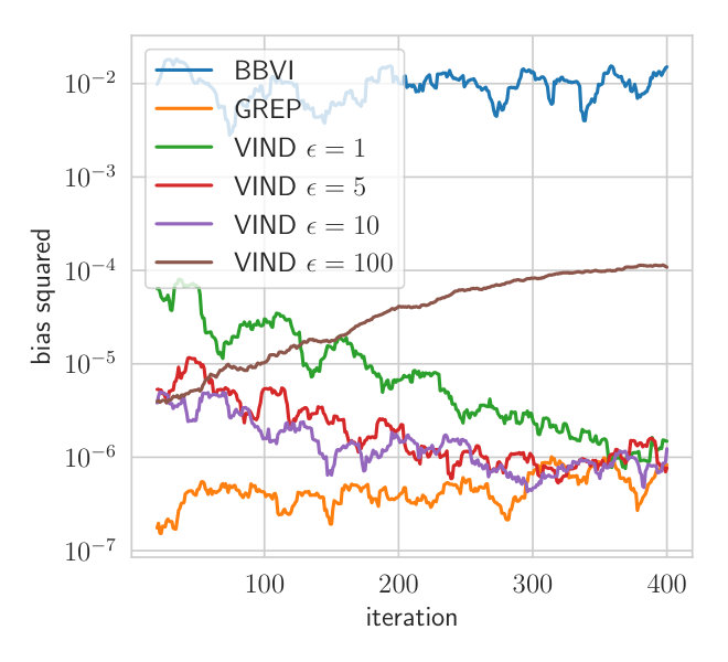 Figure 1
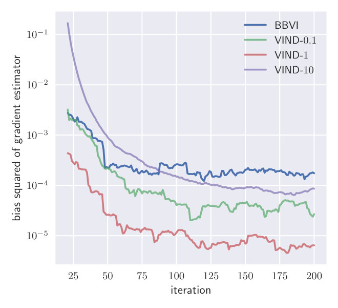 Figure 2
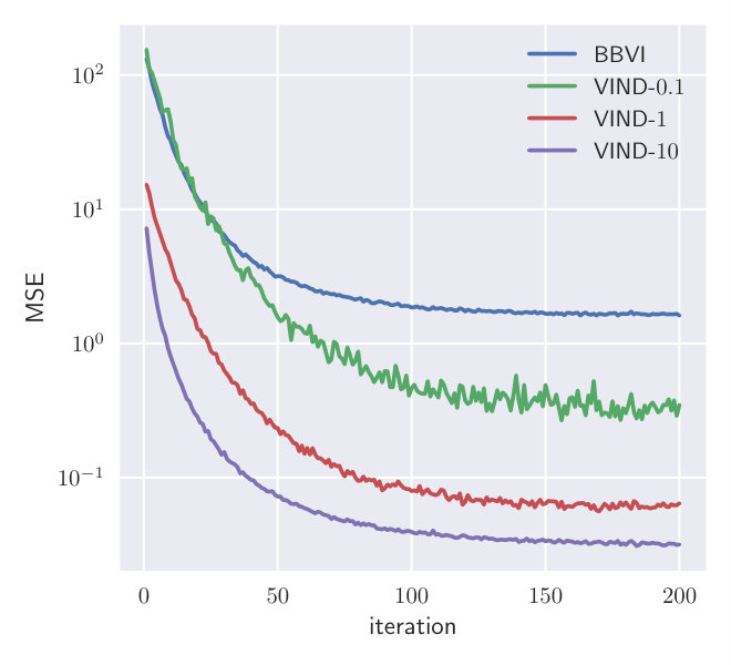 Figure 3
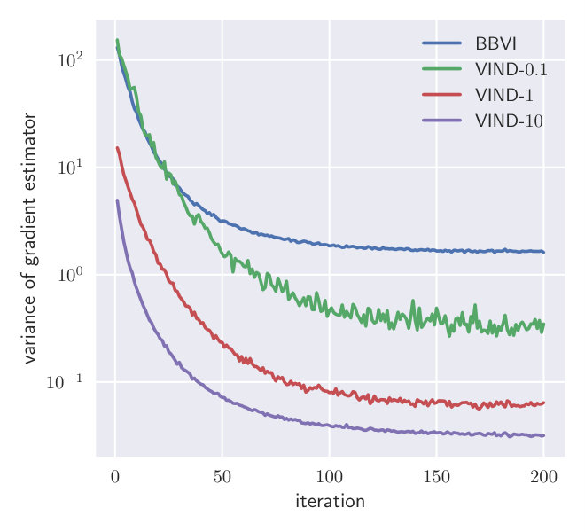 Figure 4
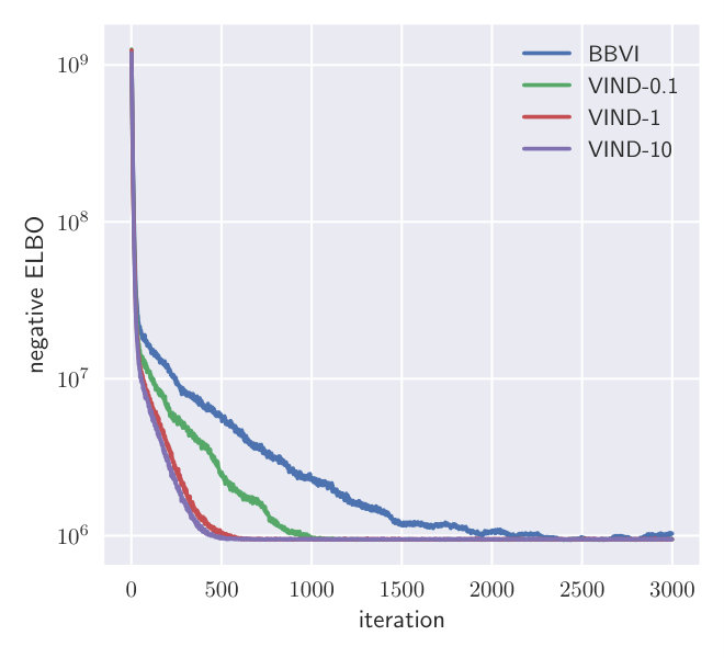 Figure 5
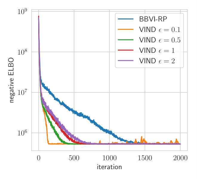 Figure 6
 Figure 7
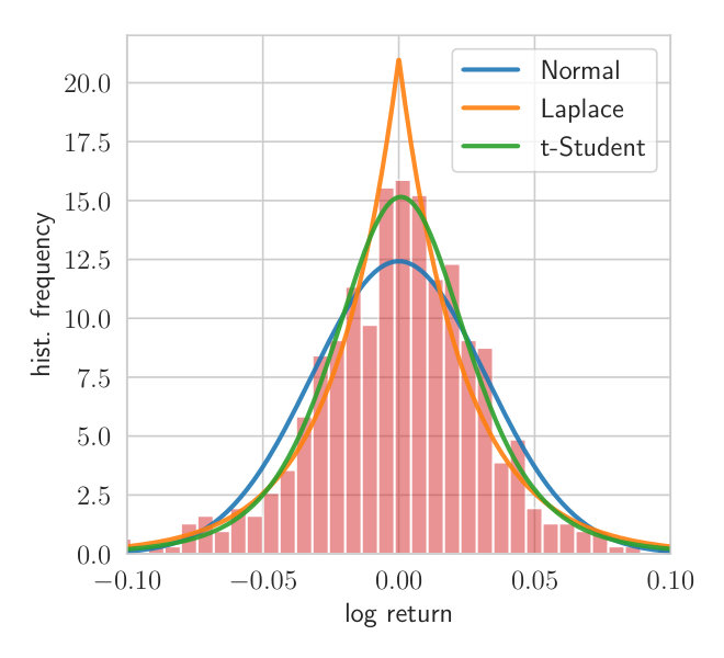 Figure 8
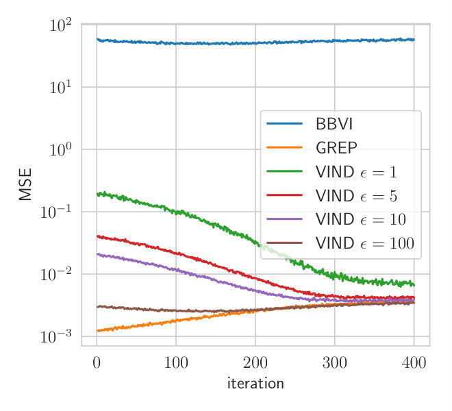 Figure 9
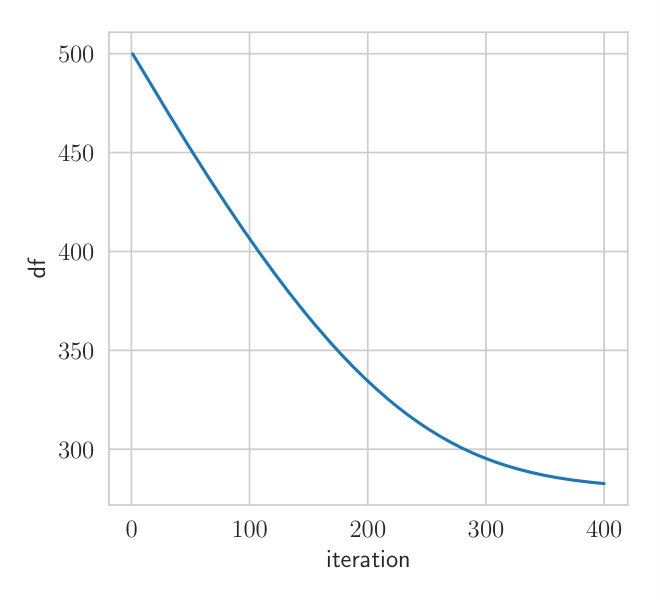 Figure 10
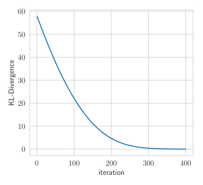 Figure 11
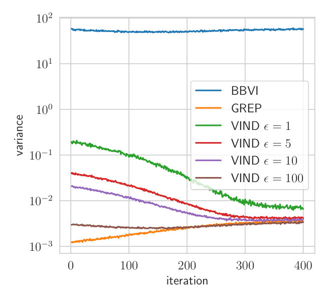 Figure 12
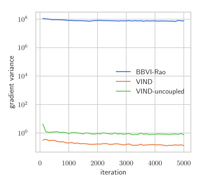 Figure 13
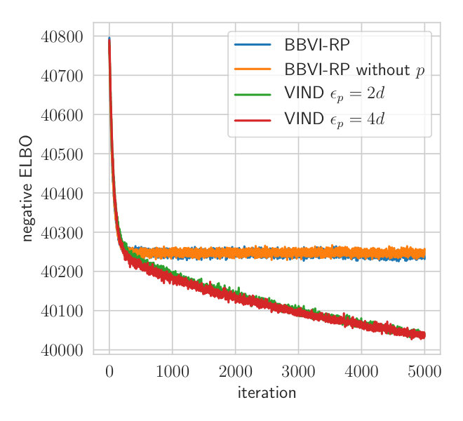 Figure 14
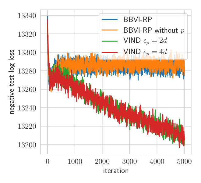 Figure 15
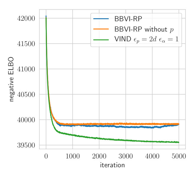 Figure 16
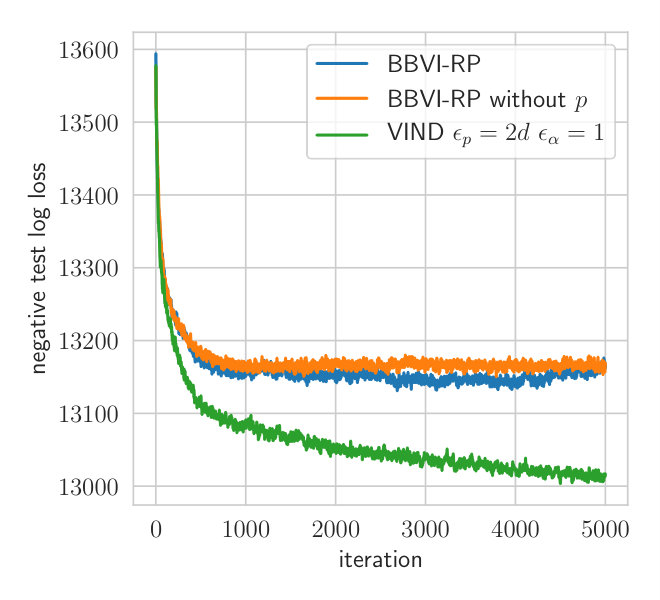 Figure 17
Peer Reviews
No public reviews on file for this paper yet. If you reviewed it on a platform where reviews are public (OpenReview, ICLR, NeurIPS, ICML), you can paste yours below so the community can read it here.
Code & Models
Videos
No videos yet. Explain this paper in a talk, walkthrough, or lecture? Add one.
Taxonomy
TopicsGaussian Processes and Bayesian Inference · Generative Adversarial Networks and Image Synthesis · Stochastic Gradient Optimization Techniques
MethodsSPEED: Separable Pyramidal Pooling EncodEr-Decoder for Real-Time Monocular Depth Estimation on Low-Resource Settings
Variational Inference with Numerical Derivatives: variance reduction
through coupling
Alexander Immer
EPFL
Guillaume Dehaene
EPFL
Abstract
The Black Box Variational Inference (Ranganath et al. (2014)) algorithm provides a universal method for Variational Inference, but taking advantage of special properties of the approximation family or of the target can improve the convergence speed significantly. For example, if the approximation family is a transformation family, such as a Gaussian, then switching to the reparameterization gradient (Kingma and Welling (2014)) often yields a major reduction in gradient variance. Ultimately, reducing the variance can reduce the computational cost and yield better approximations.
We present a new method to extend the reparameterization trick to more general exponential families including the Wishart, Gamma, and Student distributions. Variational Inference with Numerical Derivatives (VIND) approximates the gradient with numerical derivatives and reduces its variance using a tight coupling of the approximation family. The resulting algorithm is simple to implement and can profit from widely known couplings. Our experiments confirm that VIND effectively decreases the gradient variance and therefore improves the posterior approximation in relevant cases. It thus provides an efficient yet simple Variational Inference method for computing non-Gaussian approximations.
1 Introduction
Variational methods offer a promising path towards making Bayesian inference feasible for fitting large models to large datasets (Blei et al. (2017)). Indeed, a generic strategy exists to approximate a posterior distribution inside any parametric family. Ranganath et al. (2014) give the BBVI (Black Box Variational Inference) formula for a stochastic gradient of the ELBO which can then be plugged into any stochastic optimization algorithm. However, replacing this generic stochastic gradient by taking advantage of the structure of the approximating can yield a considerable reduction of the variance thus speeding up the convergence considerably. For example, when the approximating family is a transformation family (e.g. Gaussian approximations), the “reparameterization” stochastic gradient (Kingma and Welling (2014)) can be used instead.
In this article, we propose an extension of the reparameterization gradient to more general families. Our algorithm, VIND (Variational Inference through Numerical Derivatives) approximates the gradient using finite differences. By “coupling” or correlating the two approximations at which we compute the ELBO, we achieve a large reduction in variance compared to the BBVI gradient thus considerably improving the convergence. We demonstrate how to derive such couplings for Gamma, Beta, Dirichlet, Wishart, univariate and multivariate Student and Poisson approximations of the posterior distribution (Appendix Section D). In our experiments111Code available at https://github.com/AlexImmer/VIND., the VIND gradient improves upon the BBVI gradient. Indeed, we found that the BBVI gradient is unable to optimize the degree-of-freedom parameter of a Wishart approximation while VIND efficiently finds the optimal value.
2 Background
Throughout this article, we will consider the problem of computing a variational approximation of a target probability density: . We seek to find the distribution which, inside a parametric family , maximizes the Evidence Lower BOund (ELBO). This yields both the best ELBO-based approximation of the normalization constant of and the best approximation of the normalized density within the family, as measured by the KL divergence (Blei et al. (2017)). The ELBO has two alternative expressions:
[TABLE]
where is the entropy of a random variable with density .
The ELBO can always be optimized through Stochastic Gradient Descent. Indeed, the gradient of the ELBO with respect to is (Ranganath et al. (2014)):
[TABLE]
This expected value can be approximated by sampling from . The resulting stochastic optimization algorithm is referred to as Black Box Variational Inference (BBVI) to highlight the absence of any condition on the approximating family.
However, we can often take advantage of the structure of the approximation family. One particularly nice case is when we consider a transformation family, i.e. when the variable with distribution can be rewritten as a deterministic transformation of a base random variable :
[TABLE]
For example, all Gaussians can be rewritten as an affine transformation of a standard Gaussian. This structure greatly simplifies the evaluation of the gradient of the ELBO. Rewriting the ELBO as an expected value under and denoting the Jacobian matrix with , the gradient against becomes:
[TABLE]
which can once again be evaluated by sampling from . Critically, shifting from the general form (eq.(3)) to the reparameterization form of the gradient (eq.(5)) results in a major decrease of variance (Kingma and Welling (2014); Ruiz et al. (2016)). Intuitively, this makes sense since we have replaced an optimization over the space of probability distributions (eq.(3)) by an optimization over deterministic transformations of . (eq.(5)).
However, many approximation families are not amenable to a full reparameterization. For example, Gamma distributions:
[TABLE]
are only partially reparameterizable: the parameter is an inverse-scale and can thus be absorbed into a linear reparameterization but it is impossible to do so for the parameter. For families with such parameters, we propose to replace BBVI by a finite difference scheme, while doing a standard reparameterization gradient on all other parameters. By considering a sampling approximation of the ELBO at and , we obtain an alternative to the BBVI ELBO gradient (eq.(3)):
[TABLE]
However, independent sampling from and would yield a larger variance than necessary. Instead, we propose to sample from a coupling of these two distributions: a heavily correlated joint distribution such that its marginals are and (Thorisson (1995); Villani (2008); see Propp and Wilson (1996) for an application to MCMC sampling). Comparison between and is then easy: it suffices to compare the empirical mean under the samples to the mean under the samples.
Ruiz et al. (2016) propose instead to tackle such parameters by performing an approximate reparameterization. More precisely, they propose to standardize (or a transformation of it) so that it has mean [math] and covariance the identity matrix. For example, for the Gamma approximation, they propose to standardize :
[TABLE]
The resulting standardized variable has a distribution that does not depend on and has a weaker relationship to than : the conditional mean of is constant while the conditional mean of is roughly equal to . The gradient of the ELBO then decomposes into a reparameterization term and a BBVI remainder term and has a smaller variance than the standard BBVI gradient (Ruiz et al. (2016)). This Generalized Reparameterization gradient (GREP) is directly parallel to VIND in that it tries to extend the good properties of the reparameterization gradient to families which do not possess a transformation family structure. However, one sharp limit of GREP is that it is highly non-trivial to derive appropriate standardizations of a given approximation family.
Another possibility to minimize the variance consists of using control variates (see Geffner and Domke (2018) and the references therein). This approach minimizes the variance by identifying functions of which have a known expected value and which can closely approximate the log-ratio . The ELBO can then be decomposed into a deterministic term and smaller stochastic remainder thus minimizing the variance. While control variates approaches are necessary to get the optimal variant of a stochastic optimization method, it is orthogonal to ideas such as VIND which aim to radically modify the form of the gradient. We will investigate in further work how to properly combine VIND with control-variates methods in order to achieve maximal efficiency.
3 Variational Inference with Numerical Derivatives
Computing gradients with finite differences is simple and intuitive. We just vary the parameter by while computing the loss to get an approximation of the gradient. This yields an approximation of the gradient that is accurate up to errors. For example, if the parameter is one dimensional, we can approximate the gradient as:
[TABLE]
where are random variables with distribution . The VIND update is a slight refinement of eq.(10) which computes the density of the approximation at parameter value instead of :
[TABLE]
This modification ignores a term with gradient equal to [math]. Ignoring this term thus reduces the variance while still yielding an approximation of the gradient (Appendix Section B). Please notice that eq.(11) requires that both values correspond to valid parameterizations so that we can sample from both and . This might require tuning the value of to or to perform one-sided finite-differences approximations instead when is close to the edges of the parameter space.
As in BBVI and the reparameterized form of the ELBO, the gradient approximation (eq.(11)) can be evaluated through sampling from . This is non-trivial as sampling independently from these two distributions generally yields a high-variance gradient estimator (Appendix Fig.5). The key trick consists instead of sampling from a coupling (Thorisson (1995); Villani (2008)):* *a joint distribution such that and are marginally respectively distributed from . There are infinitely many such couplings with the independent coupling being the simplest one. For a finite-difference approximation of the gradient, it is more efficient for to have high-positive correlation. Indeed, consider the term in the ELBO. The variance of the corresponding approximation of the gradient is:
[TABLE]
which is minimized when and are highly positively correlated.
The variance of the gradient determines the convergence speed and the possible obtainable minimum loss (Bottou (1998); Duchi et al. (2011); Kingma and Ba (2014)). In VIND, the variance depends on our choice of and the particular coupling that we use. Larger values of typically lead to smaller variance but they also lead to the numerical approximation of the derivative of the ELBO becoming rougher. It is not a priori clear which choice is optimal. Our experiments indicate that the range of values of acceptable values of is large (Fig. 1).
3.1 Coupling the Gamma distribution
Let us now show how we can achieve a coupling with high covariance for the Gamma distribution (see Appendix Section D for coupling of other families). The family of Gamma distributions has a key property: the sum of two Gamma variables with the same is still a Gamma variable. Mathematically, for any , we have:
[TABLE]
Furthermore, the parameter is amenable to reparameterization since it is a inverse-scale parameter. It is thus straightforward to express to construct a coupling of , reparameterized in , using three auxiliary Gamma variables as:
[TABLE]
Given independent samples from this coupling , we can evaluate the gradient of the ELBO against with the reparameterization formula (eq.(5)):
[TABLE]
while the gradient against can be approximated through the VIND formula (eq.(11)):
[TABLE]
3.2 General formulation
The general procedure of the VIND algorithm is as follows. In order to compute a variational approximation of inside a given parametric family , we need to first identify all the parameters that are not amenable to normal reparameterization and for which we desire to compute a VIND gradient. For every such parameter , we need to construct a joint distribution of and where the coordinate of has been perturbed by epsilon. Finally, the VIND approximation of the gradient to is constructed and then approximated using samples from the coupling :
[TABLE]
Thus, in order to extend this approach to other approximation families, we need to devise an appropriate coupling. In the Appendix, we give couplings for the Gamma, Beta, Dirichlet, Wishart, univariate and multivariate Student and Poisson distributions (Appendix Section D).
The VIND algorithm generalizes the reparameterization gradient. Indeed, transformation families have a straightforward coupling which is such that the VIND gradient coincides to the reparameterization gradient in the limit (Appendix Section C). These two methods should thus be similar. While we have not been able to provide theoretical reasons for the VIND gradient to have a smaller variance than the BBVI gradient, we believe that the following heuristic explanation might provide some insight. The reparameterization gradient is able to improve upon BBVI by providing a simpler comparison between the ELBO at various values of . Instead of comparing how the expected value under is modified, we seek instead the best deterministic transformation of a base variable through the mapping . This modifies the space on which we are optimizing from the complicated space of probability distributions to the simpler space of deterministic deformations of a base probability distribution. The VIND idea expands upon this idea of finding the best deformation except we further consider stochastic deformations in order to deal with families which do not have the transformation family structure.
4 Experiments
We apply VIND to both synthetic and real-world problems and compare it to the standard BBVI approach (Ranganath et al. (2014)) and the generalized reparameterization gradient of Ruiz et al. (2016) (GREP). We use synthetic data and a conjugate model to showcase the variance reduction compared to BBVI and highlight the influence of different values of the hyperparameter . Further, we compare VIND to BBVI on a covariance estimation problem for financial data where the approach of Ruiz et al. (2016) cannot be applied. Throughout this section, we use Adam as the gradient descent routine with standard parameters (Kingma and Ba (2014)) but adjusted learning rates per parameter. In Appendix Section A, we provide additional details and an additional application to linear regression.
4.1 Gradient MSE in a Gamma-Normal model
To investigate the mean-squared error of the VIND gradient estimator, we use a synthetic set of data sampled from a univariate Gaussian distribution of known mean [math], i.e. . We want to find the posterior over . The conditional distribution is a Gaussian with fixed mean and the prior is a Gamma distribution. Due to conjugacy of this model, we have access to the actual gradient and can estimate the variance and bias of the VIND and BBVI gradients. The conditional model and prior are defined as follows:
[TABLE]
We approximate the true posterior with a Gamma distribution . is the variational parameter to fit while the rate is set to the posterior parameter according to the conjugate model. This is done to focus on the parameter which cannot be optimized through a reparameterization gradient. We optimize the ELBO using the true gradient. At each step, the gradient mean-squared error (MSE) is estimated for VIND with different values of and BBVI. Both methods use two samples per gradient estimate.
Fig.1 depicts the MSE of different gradient estimators. The gradient obtained using VIND yields a lower MSE for a wide range of values for compared to the BBVI gradient. This experiment shows that the VIND update provides a massive reduction in variance compared to BBVI, comparable to that achieved by Ruiz et al. (2016) while the bias is negligible compared to the variance.
4.2 Covariance Estimation for Financial Data
We further considered a data set of weekly log returns of the Dow Jones in the period from 2011 to 2018. Data is obtained for weeks and of the 30 companies constituting the Dow Jones as 2018 (for a list of stock symbols see Appendix Section A.2)222The historical data are obtained from https://finance.yahoo.com.. We denote the data set by with . The data pass a stationarity and autocorrelation test, i.e. it is reasonable to assume fixed mean and variance. We conduct a wavelet spectrum test to account for second order stationarity (Nason (2013)) and the Durbin-Watson test to exclude autocorrelation (Durbin and Watson (1950, 1951)).
To apply portfolio optimization models that trade off risk and return, both mean and covariance of the options need to be estimated (Ryan (2006)). Bayesian methods have the advantage over frequentist methods that we have access to the parameter uncertainty. However, the only conjugate model available assumes the data to be distributed according to a Gaussian. For a more elaborate model, one therefore usually resorts to approximate inference.
We treat this as a classical Bayesian multivariate location-scale estimation problem. For the conditional, we choose a t-Student distribution (i.e. the marginal distribution of a multivariate Gaussian variable divided by a variable, where is the degree of freedom parameter of the Student) modeling the possibility of major deviations from the mean that are almost impossible under a Gaussian model. The additional degree of freedom parameter allows fitting the shape more closely. We denote the multivariate t-Student distribution as parameterized by mean, shape, and degree of freedom (). We place a spherical Gaussian prior on with zero mean and a Gamma prior on with density concentrated in the range between 1 and 10. We place an uninformative Wishart prior on as it is commonly used on these tasks (Leonard et al. (1992); Alvarez et al. (2014). We perform mean-field variational inference, i.e. we consider an approximating family which factorizes as:
[TABLE]
where denotes the Wishart distribution. This approximate family is appropriate since it would be conditionally conjugate under a Gaussian conditional model of the . More generally, the Wishart distribution seems the natural choice of approximating family for symmetric positive matrices because it has an explicit density and we can sample from it. For and , the reparameterization trick can be applied to obtain the gradient. For and , we compare the impact of gradients estimated by VIND and BBVI. While it would be possible to apply the GREP gradient to , there is no simple approximate standardization available for . We thus were unable to use the GREP gradient to optimize . For VIND, we use and for the variational parameters and , respectively.
Fig. 2 shows the convergence behavior of both methods. is initialized to the conjugate parameter according to a Wishart-Normal model while all other parameters are initialized with the prior parameters. This ensures that the initial approximate posterior of is concentrated around the empirical covariance of the data. Both methods are applied with three samples per iteration, which is the minimum for VIND.
Due to the reduced variance of the VIND gradient, we can attain a higher ELBO on this task. Note that the BBVI’s gradient of is so noisy that it hardly improves the ELBO compared to keeping fixed (Fig.2). The BBVI method thus completely fails in this example since it is unable to tune the variability of the Wishart approximation of the posterior distribution of . The computation time of VIND and BBVI is the same. We further measure the variance of the VIND and BBVI gradient (Appendix Section A.2), which shows that VIND exhibits gradients that have orders of magnitude less variance just like in the synthetic experiment (Section 4.1).
5 Discussion
From our experiments, it appears that VIND provides an efficient way to find the best variational approximation in families for which the reparameterization trick is inapplicable but for which there exists a coupling. While it does require identifying a tight coupling of , we have provided such couplings for a wide variety of approximation families (Appendix Section D). The VIND gradient thus provides a major improvement over the BBVI baseline that remains competitive with the GREP gradient (Ruiz et al. (2016)) while having a much simpler derivation.
A key limit of VIND is that it scales poorly when it is used to compute the gradient over many parameters, a key limit of numerical approximation of gradients. This restricts its usage to approximating families for which most parameters are amenable to reparameterization and for which VIND is only used for a handful of key parameters. This is a key feature of the Gamma and Wishart distributions for which only one scalar parameter cannot be reparameterized. Indeed, in order to evaluate a gradient against parameters using numerical derivatives, we need to evaluate the function at positions. Constructing a coupling on this space will require many more random samples than the usage of the BBVI gradient. In approximating families with a large number of parameters that are not amenable to reparameterization, the GREP gradient from Ruiz et al. (2016) should thus be preferred.
However, we believe that this should be sufficient in the context of simple statistical models (i.e. excluding Variational Auto-Encoders and other models for which the posterior has a very complicated structure). Indeed, if we have sufficiently many datapoints then, under mild assumptions on the data and model, we should expect from a heuristic interpretation of the Bernstein-von Mises theorem (Van der Vaart (2000); Kleijn et al. (2012)) that the posterior distribution has a Gaussian limit. The family of Gaussians thus has theoretical backing that other approximations lack while also being amenable to reparameterization in all of its parameters. Since it wins on both the theoretical and computational fronts, it thus seems sensible to use the family of Gaussians as a default approximation from which we should only deviate in key parameters, such as when a conjugate prior would exist in a simpler model of the data as was the case in our financial data application.
We have presented in this article how to apply VIND when the approximating family is either Gamma, Beta, Dirichlet, Wishart, univariate and multivariate Student or Poisson (Appendix Section D). VIND is thus applicable to a wide variety of critical approximation families. Extending the algorithm further will be the subject of additional work, but this seems to be a hard task since it requires the identification of simple yet tight couplings of the various members of the family.
The key idea of VIND, using a coupling to minimize the variance of the stochastic gradient, might also provide an interesting alternative to existing algorithms for the maximization of the multi-sample ELBO (Cremer et al. (2017); Domke and Sheldon (2018)). Another possible extension for VIND is the integration of additional variance reduction techniques such as control variates (Geffner and Domke (2018)) or Rao-Blackwellization (Ranganath et al. (2014)). We will investigate this in further research.
Appendix A Details of experiments
In this appendix, additional experimental results and details are listed. Apart from further details on the experiments in the main text, we present another benchmark using a standard linear regression model, a real-world extension of the synthetic Gamma-Normal model (Section 4.1).
A.1 Synthetic Gamma-Normal Model
In Section 4.1, we showed that the MSE of the estimated gradient can be much lower using VIND compared to BBVI. Due to the use of a conjugate model, we can compute both the variance and bias of the estimators. We claimed that despite the finite difference approach, VIND shows almost no bias and the variance of the estimated gradient dominates the MSE. Figure 3 displays the variance and bias along the ascent path of the true gradient of the ELBO in the Gamma-Normal experiment. Due to the high variance of the BBVI gradient, the estimated bias is actually higher than that of some VIND estimators. The variance is at least four orders of magnitude larger than the bias, which supports our hypothesis that the eventual bias of VIND is negligible and the variance reduction has a high impact.
A.2 Wishart Student Financial Application
We provide additional details of our financial application. The symbols of the stocks used are the following: *AAPL, AXP, BA, CAT, CSCO, CVX, DIS, DWDP, GE, GS, HD, IBM, INTC, JNJ, JPM, KO, MCD, MMM, MRK, MSFT, NKE, PFE, TRV, UNH, UTX, V, VZ, WMT, *and XOM. These stocks are 29 of 30 companies in the Dow Jones as of May 2018. The conjugate Gaussian model cannot provide a sufficiently close fit to the data, as illustrated in Figure 4. This figure shows the histogram for 510 weeks of data and the maximum likelihood fits using the Normal, Laplace, and t-Student distribution. The Laplace and Normal distributions fit poorly in the tails whereas the t-Student can fit the shape of the histogram due to the additional degree of freedom.
As pointed out in Section A.2, we start all variational parameters from the prior parameters except for For we compute the empirical covariance of the data, invert it and divide it by the initial parameter for The expected value of the Wishart distribution is thus the empirical precision matrix. This reduces the number of iterations until convergence and highlights the final convergence. The results are reproducible with different optimization procedures (e.g. Adagrad) and various initialization parameters. BBVI can only attain a comparable maximum ELBO if the degree of freedom of the posterior Wishart distribution is initialized to the optimum reached using VIND.
Similar to the synthetic experiment presented in Section 3, we estimate the variance of different gradient estimators for this model. Having no access to the true gradient, we can only estimate the variance. Figure 5 shows the variance of VIND, VIND without coupling, and BBVI with Rao-Blackwellization along the descent path of VIND. The gradient estimates using BBVI have a much higher variance than those of VIND. VIND without coupling has approximately one order of magnitude higher variance but is still a better solution than BBVI on this problem. The high gradient variance leads to the inability to properly converge in the variational parameter which is apparent in Figure 2 in Section A.1.
A.3 Linear Regression
The synthetic example with a Gamma-Normal model has shown that VIND can estimate gradients with much lower variance compared to BBVI. A common application of the Gamma distribution arises in a linear regression setting. We observe a set of feature vectors paired with a real quantity to predict, i.e. we have the data set and with and . We use the Boston Housing benchmark data set with and . We center and standardize the features and further decorrelate them using principal component analysis. We have the following conditional model and prior, respectively:
[TABLE]
We would have a conjugate model if the prior was hierarchical, i.e. . With the independent prior, we need to resort to approximate methods such as variational inference. The approximating family is of the same structure as the prior (mean-field) and, with , is given by
[TABLE]
The prior parameters are and we have a cold start on all parameters with . Figure 6 depicts the convergence of the negative ELBO for VIND with different values of epsilon and BBVI. The procedure converges much faster using the gradient estimated with VIND. Using , VIND converges after around 500 iterations while BBVI requires approximately 2500. In comparison to the Wishart-Student model analyzed in Section A.2, BBVI can attain the same loss as VIND but requires much more time to do so.
Appendix B Derivation of the VIND update
Let us now derive in detail the precise form of the VIND gradient and why it differs from the immediate numerical approximation of the gradient of the ELBO.
Throughout this section, we assume that we are dealing with a one-dimensional parameter approximation family: . The argument is straightforward to extend to the higher-dimensional case.
The numerical approximation of the derivative of the ELBO is:
[TABLE]
In the limit , a Taylor expansion of the ELBO centered at yields that this approximation is exact up to order if the ELBO is differentiable three times:
[TABLE]
However, the naive numerical approximation of the derivative is slightly suboptimal. This can be shown by a Taylor expansion of around . For all , we have:
[TABLE]
We thus have:
[TABLE]
The extra term is actually equal to since the expected value of the gradient is [math]:
[TABLE]
We have thus established that the difference between the true numerical approximation of the derivative of the ELBO (eq.(10)) and the VIND approximation (eq.(11)) corresponds to the numerical approximation of a term with derivative [math]. It is thus more efficient to use the VIND approximation of the gradient which deliberately sets this term exactly to [math]. This is compounded by the result in the next Section which establishes that the VIND update coincides with the reparameterization gradient in a transformation family. This would not be true for the true numerical approximation of the derivative of the ELBO in which there is an extra term present which is exactly .
Appendix C Linking VIND to the reparameterization gradient
If is a transformation family, then the VIND gradient is almost equal to the reparameterization gradient, as we now show.
First, let us build the straightforward coupling of and . We do so by using the transformation family property:
[TABLE]
where the distribution of is fixed.
The VIND approximation of the gradient of the ELBO is then:
[TABLE]
which simplifies in the limit . Indeed:
[TABLE]
Thus yielding:
[TABLE]
We thus finally have:
[TABLE]
which is exactly the expression of the reparameterization gradient of the ELBO.
Appendix D Couplings
In this section, we detail how to derive the VIND gradient to find an approximation of the target distribution in the Gamma, Beta, Dirichlet, Wishart, univariate and multivariate Student or Poisson families. For each of those families, we detail a coupling a construction of and for all parameters which are not amenable to a reparameterization and we give a reparameterization transform for all other parameters.
Please notice that, throughout this section, we do not take advantage of the fact that the entropy of most of those distributions is explicit (i.e. we use eq.(1) to define the ELBO). All the following formulas thus have a variant where only the terms in remain and the terms of depending on are replaced by an explicit gradient , based on eq.(2). This alternative formula could yield improvements on the variance of the estimator depending on the circumstance through the use of control variates (Geffner and Domke [2018]).
D.1 Gamma distribution
Consider the family of Gamma distributions. The conditional density is:
[TABLE]
The parameter is an inverse-scale parameter and thus has a standard reparameterization gradient. The parameter needs to be handled instead with a VIND gradient through the following coupling:
[TABLE]
This coupling leverages the key fact that a sum of two Gamma random variables with the same scale parameter is also a Gamma random variable. The alpha parameter of the sum is equal to the sum of the alpha parameters of the summands.
Given independent samples from this coupling , the VIND gradient is:
[TABLE]
D.2 Beta distribution
Consider the family of Beta distributions. The conditional density is:
[TABLE]
Both parameters need to be handled through a coupling construction. We leverage here the key fact that a Beta random variable can be constructed as the ratio of two gammas:
[TABLE]
From this, we can construct a coupling of and in the following way. First, we construct :
[TABLE]
This construction yields the following VIND gradient:
[TABLE]
D.3 Dirichlet distribution
The Dirichlet distribution is a distribution over a -dimensional random variable with density:
[TABLE]
It is supported on the -dimensional simplex defined as the ensemble of points such that and for all coordinates .
Exactly like the Beta distribution, the Dirichlet distribution can be constructed as a ratio of Gamma random variables. More precisely, given Gamma random variables:
[TABLE]
then the random variable with coordinates:
[TABLE]
follows a Dirichlet distribution with parameters .
Thus, we can construct a coupling by first generating Gamma random variables:
[TABLE]
The variable and its distorted variants are then straightforward to compute:
[TABLE]
The VIND gradient is then straightforward to derive and matches that of the Beta distribution.
D.4 Wishart distribution
The Wishart distribution is a distribution over the space of positive matrices of shape . It has two parameters: the degree of freedom and the scale matrix which is a strictly positive matrix of shape . Let denote a Wishart random variable. Its density is:
[TABLE]
where is the determinant of the matrix and is the trace operator.
The Wishart distribution is the matrix equivalent of the Gamma distribution. The parameter can be handled through a reparameterization while the degree of freedom parameter requires a coupling construction. The coupling construction is made possible by the fact that the sum of two Wishart random variables with identical scale but different degrees of freedom and is another Wishart variable with scale and degree of freedom .
Let where is a symmetric matrix. We propose the following coupling:
[TABLE]
Given samples from this coupling , we have the following VIND gradient:
[TABLE]
Please notice that the gradients against and against in eq.(59a) need to take into account that both matrices are symmetric.
D.5 Univariate and multivariate Student
The multivariate Student distribution with center , scale (a symmetric matrix), and degree of freedom over has the following density:
[TABLE]
A key property of this distribution is that it corresponds to the marginal distribution of a scaled and translated ratio of a Standard normal and a chi-square variable:
[TABLE]
The marginals of this distribution are, once we center and scale them appropriately, the ordinary Student distribution.
The and parameters correspond to a center and a scale and are thus amenable to reparameterization. The parameter requires a coupling construction:
[TABLE]
which yields the VIND gradient:
[TABLE]
D.6 Poisson distribution
The Poisson distribution is a discrete distribution over with mass function:
[TABLE]
It has the key property that the sum of two Poisson random variables with rates and is another Poisson random variable with rate .
This yields the coupling:
[TABLE]
This yields the naive VIND gradient:
[TABLE]
However, this naive gradient can be improved. Indeed, it is inefficient due to the high probability of the event which yields a null gradient. It is better to first modify the VIND gradient by explicitly conditioning on the events and :
[TABLE]
which is straightforward to evaluate with a sampling approximation. We simply construct samples using the conditional distribution of when :
[TABLE]
This improved VIND gradient is more efficient since it avoids sampling from the event which provides no information concerning the sign of the gradient.
The reference list from the paper itself. Each links out to its DOI / PubMed record.
- 1Alvarez et al. [2014] Ignacio Alvarez, Jarad Niemi, and Matt Simpson. Bayesian inference for a covariance matrix. ar Xiv preprint ar Xiv:1408.4050 , 2014.
- 2Blei et al. [2017] David M Blei, Alp Kucukelbir, and Jon D Mc Auliffe. Variational inference: A review for statisticians. Journal of the American Statistical Association , 112(518):859–877, 2017.
- 3Bottou [1998] Léon Bottou. Online algorithms and stochastic approximations. In David Saad, editor, Online Learning and Neural Networks . Cambridge University Press, Cambridge, UK, 1998. URL http://leon.bottou.org/papers/bottou-98x . revised, oct 2012.
- 4Cremer et al. [2017] Chris Cremer, Quaid Morris, and David Duvenaud. Reinterpreting importance-weighted autoencoders. ar Xiv preprint ar Xiv:1704.02916 , 2017.
- 5Domke and Sheldon [2018] Justin Domke and Daniel R Sheldon. Importance weighting and variational inference. In Advances in Neural Information Processing Systems , pages 4470–4479, 2018.
- 6Duchi et al. [2011] John Duchi, Elad Hazan, and Yoram Singer. Adaptive subgradient methods for online learning and stochastic optimization. Journal of Machine Learning Research , 12(Jul):2121–2159, 2011.
- 7Durbin and Watson [1950] James Durbin and Geoffrey S Watson. Testing for serial correlation in least squares regression: I. Biometrika , 37(3/4):409–428, 1950.
- 8Durbin and Watson [1951] James Durbin and Geoffrey S Watson. Testing for serial correlation in least squares regression. ii. Biometrika , 38(1/2):159–177, 1951.