Validation and calibration of coupled porous-medium and free-flow problems using pore-scale resolved models
Iryna Rybak, Christoph Schwarzmeier, Elissa Eggenweiler, Ulrich R\"ude

TL;DR
This study validates and calibrates coupled free-flow and porous-medium models using pore-scale simulations, highlighting the importance of interface conditions and effective parameters for accurate predictions in complex geometries.
Contribution
It introduces a validation framework for coupled Stokes-Darcy models using pore-scale resolved simulations across different geometries and interface conditions.
Findings
Coupled model results are sensitive to interface location and parameters.
Effective parameters vary with geometrical configuration.
Validation improves understanding of interface condition impacts.
Abstract
The correct choice of interface conditions and effective parameters for coupled macroscale free-flow and porous-medium models is crucial for a complete mathematical description of the problem under consideration and for accurate numerical simulation of applications. We consider single-fluid-phase systems described by the Stokes-Darcy model. Different sets of coupling conditions for this model are available. However, the choice of these conditions and effective model parameters is often arbitrary. We use large scale lattice Boltzmann simulations to validate coupling conditions by comparison of the macroscale simulations against pore-scale resolved models. We analyse two settings (lid driven cavity over a porous bed and infiltration problem) with different geometrical configurations (channelised and staggered distributions of solid grains) and different sets of interface conditions.…
Click any figure to enlarge with its caption.
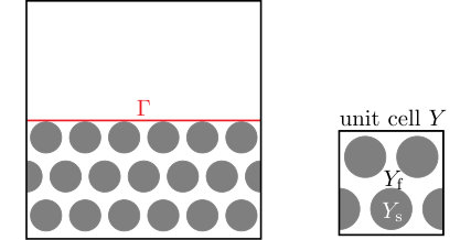 Figure 1
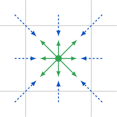 Figure 2
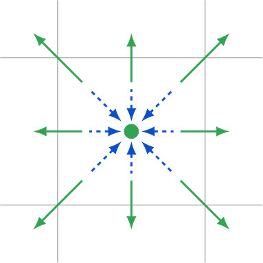 Figure 3
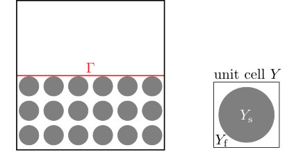 Figure 4
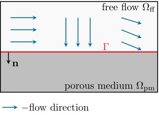 Figure 5
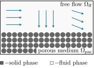 Figure 6
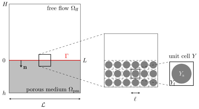 Figure 7
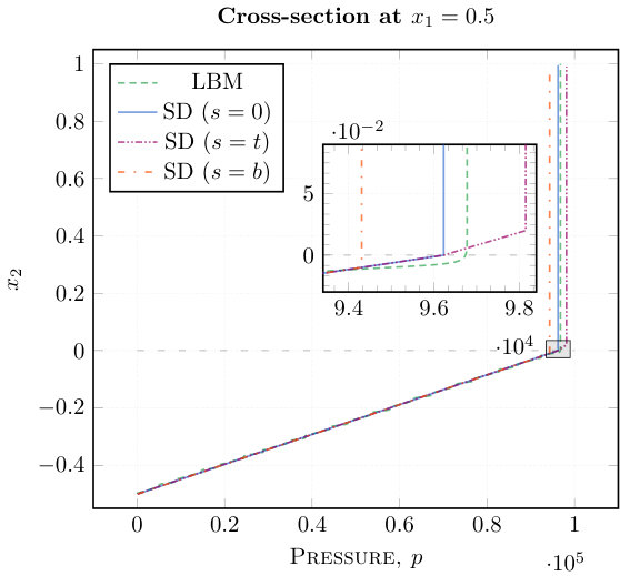 Figure 8
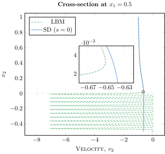 Figure 9
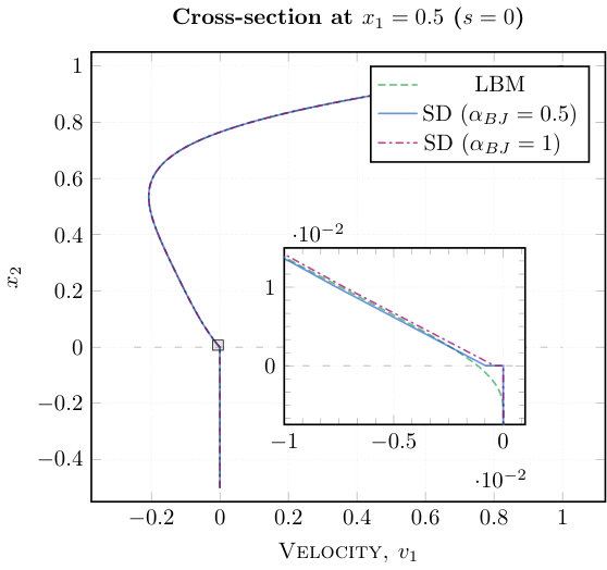 Figure 10
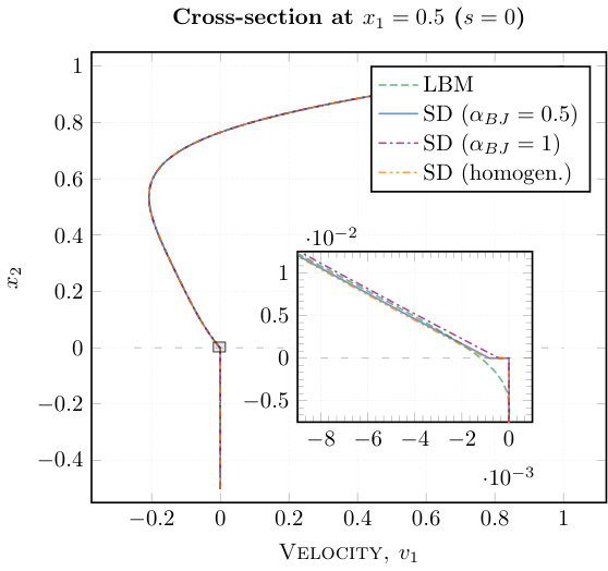 Figure 11
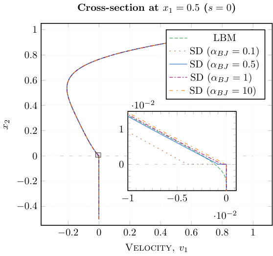 Figure 12
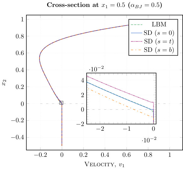 Figure 13
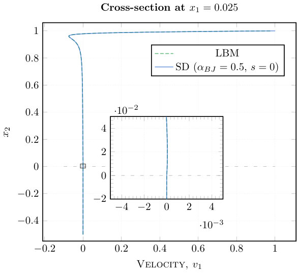 Figure 14
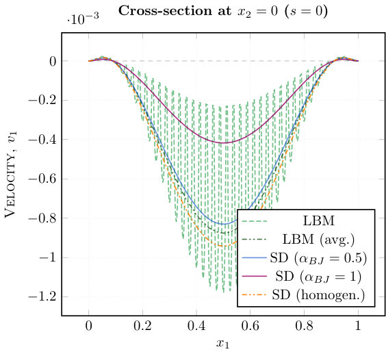 Figure 15
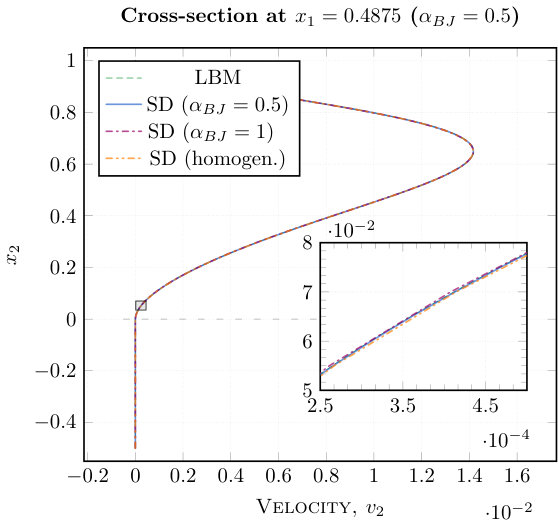 Figure 16
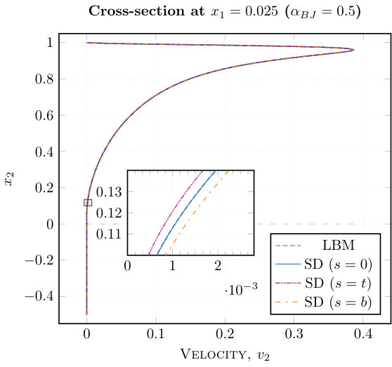 Figure 17
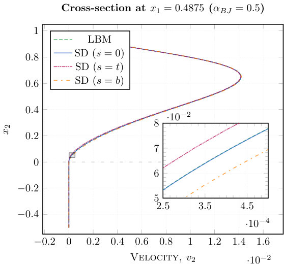 Figure 18
Peer Reviews
No public reviews on file for this paper yet. If you reviewed it on a platform where reviews are public (OpenReview, ICLR, NeurIPS, ICML), you can paste yours below so the community can read it here.
Videos
No videos yet. Explain this paper in a talk, walkthrough, or lecture? Add one.
\smartqed
11institutetext: I. Rybak 22institutetext: E. Eggenweiler 33institutetext: Institute of Applied Analysis and Numerical Simulation,
University of Stuttgart,
Pfaffenwaldring 57, 70569 Stuttgart, Germany
33email: [email protected], [email protected] 44institutetext: C. Schwarzmeier 55institutetext: U. Rüde 66institutetext: Chair for System Simulation,
Friedrich-Alexander University Erlangen-Nürnberg,
Cauerstraße 11, 91058 Erlangen, Germany
66email: [email protected], [email protected] 77institutetext: U. Rüde 88institutetext: CERFACS, 42 Avenue Gaspard Coriolis, 31057 Toulouse, France
Validation and calibration of coupled porous-medium and free-flow
problems using pore-scale resolved models
Iryna Rybak
Christoph Schwarzmeier
Elissa Eggenweiler
Ulrich Rüde
Abstract
The correct choice of interface conditions and effective parameters for coupled macroscale free-flow and porous-medium models is crucial for a complete mathematical description of the problem under consideration and for accurate numerical simulation of applications. We consider single-fluid-phase systems described by the Stokes–Darcy model. Different sets of coupling conditions for this model are available. However, the choice of these conditions and effective model parameters is often arbitrary. We use large scale lattice Boltzmann simulations to validate coupling conditions by comparison of the macroscale simulations against pore-scale resolved models. We analyse two settings (lid driven cavity over a porous bed and infiltration problem) with different geometrical configurations (channelised and staggered distributions of solid grains) and different sets of interface conditions. Effective parameters for the macroscale models are computed numerically for each geometrical configuration. Numerical simulation results demonstrate the sensitivity of the coupled Stokes–Darcy problem to the location of the sharp fluid-porous interface, the effective model parameters and the interface conditions.
keywords:
Stokes equations Darcy’s law Interface conditions Lattice Boltzmann method
1 Introduction
Coupled flow systems containing a porous-medium domain and a free-flow region appear in various environmental and technical applications, such as surface-water/ groundwater flow, industrial filtration and water management in fuel cells. The interaction between the flow regions is dominated by the interface driven processes and, due to their complexity, modelling such coupled flow systems is a challenging task.
Different spatial scales can be employed to investigate coupled free-flow and porous-medium systems. At the microscale (pore scale) the pore structure is fully resolved (Fig. 1, left) and the flow in the entire fluid domain (free-flow region and pore space in the porous medium) is described by the Navier–Stokes equations with the no-slip condition at the boundary of the solid inclusions. However, computing the microscale flow field is infeasible for practical applications as it requires detailed information about porous-medium morphology and topography which is usually unknown. Even if information on the pore structure is available, e.g., obtained from tomographic analysis Blunt_17 ; Wildenschild_Sheppard_13 or known in advance for artificially produced composite materials (GeoDict, www.math2market.com), performing microscale simulations is computationally highly demanding.
From the macroscale perspective, the whole system is described as two different continuum flow domains (free flow, porous medium) separated by an equi-dimensional transition region or a lower-dimensional (co-dimension one) sharp interface. Different mathematical models are usually used in the two flow regions. Thus, either coupling conditions at the sharp fluid-porous interface or equations that apply at the transition zone between the two flow systems are needed Beavers_Joseph_67 ; Goyeau_Lhuillier_etal_03 ; Nield_09 ; OchoaTapia_Whitaker_95 ; Saffman . Correct specification of these conditions is essential for a complete and accurate mathematical description of flow and transport processes in compositional systems as well as for an accurate numerical simulation of applications Discacciati_Miglio_Quarteroni_02 ; Discacciati_Quarteroni_09 ; Jackson_Rybak_etal_12 ; Jaeger_Mikelic_09 ; Layton_Schieweck_Yotov_03 . The Navier–Stokes equations, which in case of low Reynolds numbers can be simplified to the Stokes equations, are typically applied to describe fluid flow in the free-flow domain, while Darcy’s law or its extension is used for the flow through the porous medium. Depending on the flow regime, other models can be applied, e.g., shallow water equations or kinematic wave approximation of the Saint-Venant equation for surface flows Dawson_08 ; Sochala_Ern_Piperno_09 ; Reuter_etal_19 and the Brinkman equation, the Forchheimer equation, the Richards equation or the full two-phase porous-medium flow models for subsurface flows Brinkman_47 ; Cimolin_Discacciati_13 ; Mosthaf_Baber_etal_11 ; Rybak_etal_15 . Different sets of coupling conditions are used in the literature at the fluid-porous interface Beavers_Joseph_67 ; OchoaTapia_Whitaker_95 ; Carraro_etal_15 ; Nield_09 ; Angot_etal_17 . Some authors distinguish between two qualitatively different flow directions: near parallel flow, where the velocity of the free fluid is much larger than the filtration velocity in the porous medium and near normal flow, where velocities in the two regions have comparable magnitudes. However, these conditions cannot be applied to a general flow situation.
The macroscopic level of flow system description is the most common one used for numerical simulations of coupled systems in practical applications Arbogast_Brunson_07 ; Cimolin_Discacciati_13 ; HanspalWaghodeNassehiWakeman ; Iliev_Laptev_04 ; Mosthaf_Baber_etal_11 ; Riviere . Microscale (pore-scale resolved) numerical simulations are typically used to validate the macroscale models.
In this paper, we consider the Stokes–Darcy problem and analyse different coupling conditions at the fluid-porous interface. Most often, the conservation of mass, the balance of normal forces and the Beavers–Joseph–Saffman condition for the tangential velocity are used both for numerical analysis and simulations, e.g., Beavers_Joseph_67 ; Saffman ; Goyeau_Lhuillier_etal_03 ; Nield_09 ; Discacciati_Quarteroni_09 ; GiraultRiviere ; Layton_Schieweck_Yotov_03 ; Jaeger_Mikelic_09 . The Beavers–Joseph–Saffman condition that describes a tangential velocity slip at the fluid-porous interface was obtained for flows parallel to the porous layer. Nevertheless, this condition is often applied to other flow directions, e.g., HanspalWaghodeNassehiWakeman . Although other interface conditions are available for the Stokes–Darcy problem, they are either valid only for specific flow situations Carraro_etal_15 or contain parameters which are difficult to determine ValdesParada_etal_09 . There were also several attempts to validate the coupled models and the interface conditions, e.g., Lacis_Bagheri_17 ; Zampogna_Bottaro_16 ; Bars_Worster_06 ; Yang_etal_19 . However, to our knowledge no systematic study has been published. In this paper, we consider different interface conditions for the coupled Stokes–Darcy problem. We validate and calibrate the macroscale coupled model using pore-scale resolved numerical simulations. These fully resolved numerical simulations are performed using the lattice Boltzmann method, a numerical method for simulating fluid dynamics that is especially suited for parallel computations with high spatial and temporal resolutions in complex geometries. It thus provides first-principle insights into the physical flow processes in both domains and the flow behaviour at the interface region.
The paper is organised as follows. In Section 2 we provide the geometrical setting and the flow system description. The macroscale coupled model with different sets of interface conditions is presented in Section 3. The calculation of effective parameters for the macroscale model by means of homogenisation is discussed in Section 4 and the lattice Boltzmann method is described in Section 5. Numerical simulation results for model validation and calibration are given in Section 6. Finally, the conclusion is presented in Section 7.
2 Geometrical setting
We consider a free-flow region and a porous medium with periodic arrangement of the solid obstacles (Fig. 1, left). The fluid is considered to be present in a single phase and to fully saturate the porous medium. Additionally, it is assumed to be incompressible and to have a constant viscosity. The flow is considered as being laminar and supposing a single chemical species, no compositional effects need to be modelled. The temperature is assumed constant, such that it is not required to model any energy balance equation.
At the microscale, we solve the Stokes equations in the free-flow domain and in the pore space of the porous medium, where no-slip boundary conditions are applied on the solid-fluid boundary. At the macroscale, the system is described as two different continuum flow domains separated by the sharp interface (Fig. 1, right). We solve the Stokes and Darcy equations in the two flow domains and impose different interface conditions on the fluid-porous interface (Sect. 3). These interface conditions are validated for different porous-medium morphologies and different flow directions.
3 Macroscale coupled model formulation
Fluid flow in the free-flow region is described by the Stokes equations, the flow through the porous medium is described by Darcy’s law. Different sets of interface conditions are imposed on the sharp fluid-porous interface. Effective parameters such as permeability, porosity and boundary layer constants are needed to describe the porous-medium system and the interface conditions. These parameters are calculated in Section 6 for the geometrical configurations studied in the paper.
3.1 Free-flow model
The fluid is considered to be incompressible and therefore the mass conservation equation becomes
[TABLE]
The Stokes equation describes the fluid flow
[TABLE]
where is the fluid density, is the fluid velocity, is the pressure, is the gravitational acceleration, is the stress tensor, is the dynamic viscosity, is the rate of strain tensor and is the identity tensor.
On the external boundary of the free-flow domain , the following boundary conditions are imposed
[TABLE]
where is the unit outward normal vector from domain on its boundary and .
3.2 Porous-medium model
We consider Darcy’s flow equations in the porous-medium domain
[TABLE]
where Darcy’s velocity is given by
[TABLE]
Here is the fluid velocity through the porous medium, is the fluid pressure, is the intrinsic permeability of the porous medium, is the dynamic viscosity of the fluid, is the fluid density, is the source term and is the gravitational acceleration. The permeability tensor is symmetric, positive definite and bounded. Its values are computed numerically for the considered settings in Section 6. In this paper, we neglect gravitational effects setting .
We prescribe the following boundary conditions on the external boundary of the porous-medium domain :
[TABLE]
where is the unit outward normal vector from domain on its boundary, , , and .
3.3 Interface conditions
In addition to the boundary conditions prescribed on the external boundary of the coupled domain, a set of interface conditions has to be defined on in order to obtain a closed problem formulation. Different sets of interface conditions have been proposed in the literature depending on the flow direction.
3.3.1 Flow parallel to the interface
When the free flow is almost parallel to the porous medium, the conservation of mass, the balance of normal forces and a variation of the Beavers–Joseph condition is typically applied.
The conservation of mass across the interface is given by
[TABLE]
where is the unit normal vector at the fluid-porous interface pointing outward from the free-flow domain (Fig. 1, right).
The balance of normal forces at the interface is
[TABLE]
where .
There exist several possibilities for the interface condition on the tangential component of the velocity Nield_09 . The Beavers–Joseph interface condition Beavers_Joseph_67 for the difference between the tangential component of the free-flow velocity and the porous-medium velocity can be written as
[TABLE]
where is the Beavers–Joseph parameter, is a unit vector tangential to the interface, , and is the number of space dimensions.
Saffman Saffman simplified the Beavers–Joseph condition (9) as follows
[TABLE]
arguing that the tangential velocity of a fluid through a porous medium is small and thus can be neglected.
Jones Jones_73 considered the symmetrised rate of strain tensor in the Beavers–Joseph–Saffman interface condition
[TABLE]
Besides the classical interface conditions (7), (8) and (9)–(11), which have been formulated based on heuristic arguments and were justified experimentally, in Jaeger_etal_01 the following interface conditions on were proposed
[TABLE]
where and is the ratio of the length scales (Sect. 4). These coupling conditions are derived mathematically using homogenisation theory and boundary layer theory for flows parallel to the fluid-porous interface . The first condition in (12) differs from the classical conservation of mass condition (7). However, it seems to be reasonable for flows parallel to the porous layer, because in this case the normal component of the Darcy velocity is of order (see Eq. (18)) and thus can be neglected. The second condition in (12) links pressure fields in the porous domain and the free-flow domain, and is a variation of the classical balance of normal forces (8). The last equation in (12) is a modification of the Beavers–Joseph–Saffman law Beavers_Joseph_67 ; Saffman with . The effective coefficients and are determined through an auxiliary boundary layer problem. These coefficients and the parameter are provided for different geometrical configurations in Section 6.
3.3.2 Flow perpendicular to the interface
For flows almost perpendicular to the porous medium, the following effective interface laws on are derived in Carraro_etal_15 using the theory of homogenisation and boundary layers
[TABLE]
where is a boundary layer corrector constant. However, these conditions are valid only for a very specific setting (given geometrical configuration and boundary conditions) and cannot be applied to a general infiltration problem. There is a lack of physically consistent interface conditions for flows perpendicular to the porous layer and moreover for arbitrary flow directions.
4 Effective properties of the coupled system
To obtain effective properties for coupled macroscale models (effective permeability and boundary layer constants), we use the theory of homogenisation and boundary layers Carraro_etal_15 ; Hornung_97 ; Jaeger_Mikelic_09 . Therefore, we consider periodic porous media and assume the separation of length scales , where is the characteristic pore size and is the length of the domain of interest (Fig. 2).
We consider a coupled domain , consisting of a free-flow region and a porous medium with periodic arrangement of the solid obstacles (Fig. 1). The flow region consists of the free-flow domain , the permeable interface and the pore space of the porous-medium domain . The porous-medium geometry is defined by a periodic repetition of the scaled unit cell in (Fig. 2).
4.1 Microscale model
The fluid flow in is governed by the non-dimensional steady Stokes equations
[TABLE]
completed with the no-slip condition on the fluid-solid interface
[TABLE]
and the appropriate boundary conditions on the external boundary .
For the lid driven cavity over the porous bed described in Section 6.1, we consider
[TABLE]
and for the infiltration problem validated in Section 6.2, we have
[TABLE]
where .
4.2 Homogenisation
We obtain the corresponding macroscale formulation of the coupled system by studying the behaviour of the solutions to the microscopic problem (14)–(16) or (14), (15) and (17) when . In the limit, the equations in the free-flow region remain unchanged and we need to homogenise the porous region. To derive the limit problem in , we use the idea of homogenisation with two-scale asymptotic expansions (Hornung_97, , chap. 1 and 3):
[TABLE]
where is the fast variable. We follow the classical procedure of homogenisation to derive Darcy’s law (5) as the upscaled problem in completed by the appropriate boundary conditions.
The permeability tensor is given by
[TABLE]
where and are the solutions to the following cell problems for :
[TABLE]
The unit cell is presented in Figure 2. To obtain the effective permeability , the tensor has to be scaled with .
5 Lattice Boltzmann method
The lattice Boltzmann method (LBM) is a modern approach for simulating fluid dynamics. While the LBM historically evolved from lattice gas automata Wolf-Gladrow_00 , it can be regarded as a special discretisation of the continuous Boltzmann equation He_97 that describes the dynamics of a gas on a mesoscopic scale. On a macroscopic scale, however, the Boltzmann equation leads to the equations of fluid dynamics, i.e., mass, momentum and energy conservation. Therefore, by solving the Boltzmann equation for certain scenarios, one can also obtain the corresponding solutions to the Navier–Stokes equations Krueger_LBM .
5.1 Advantages
In comparison to conventional methods for simulating fluid dynamics, such as the finite difference, finite volume or finite element method, the LBM’s main advantages lay in its ease of implementation and its suitability for complex flow scenarios. As the most compute-intensive operations are local, i.e., restricted to neighbouring lattice cells, the LBM is inherently applicable for massively parallel computing. Furthermore, the LBM is well-suited for simulating particulate flows Rettinger_17 ; Kuron_16 , multi-phase flows Huang_15 and flows through complicated geometries such as porous media Fattahi_etal_16 ; Fattahi_etal_16b .
5.2 Description
Our introduction to the LBM follows Krueger_LBM ; the interested reader is referred to this reference and the references therein. The LBM’s most fundamental quantities are the so-called particle distribution functions that represent the density of virtual particles with velocity at position and time . The index in refers to the corresponding index of velocity in a discrete set of velocities with weighting coefficients .
Velocity sets are denoted as DQ with being the number of spatial dimensions and referring to the velocity set’s number of velocities. Velocity sets are a trade-off between accuracy and memory consumption. Different velocity sets and their corresponding coefficients can be found in the LBM literature such as Krueger_LBM . Here we limit ourselves to two spatial dimensions such that we use the well-established D2Q9 velocity set. In each velocity set, the constant determines the relation between the fluid pressure and the fluid density as . Due to this relation, is called the lattice speed of sound. In most velocity sets used to solve the Navier–Stokes equations, it can be expressed as .
The distribution function is only defined at discrete points in a square lattice with lattice spacing . Since the LBM’s origins lay in lattice gas automata, these discrete points are also often referred to as lattice cells. Similarly, is only defined at discrete times with time step . As it is common in the LBM literature, we use lattice units which is an artificial set of units that is scaled such that the relations and hold.
In kinetic theory, one obtains the macroscopic mass and momentum density by taking the moments of the Boltzmann equation’s distribution functions. Similarly, one can find the mass density and the momentum density with fluid velocity by
[TABLE]
The lattice Boltzmann equation
[TABLE]
describes the advection of particles that travel with velocity to a neighbouring lattice cell in the next time step (Fig. 3, left). After having moved from one lattice cell to another, the particles are affected by a collision operator that models particle collisions by redistributing particles among (Fig. 3, right).
The simplest collision operator that can be used for solving the Navier–Stokes equations is the Bhatnagar–Gross–Krook (BGK) operator. It linearly relaxes particle distributions towards an equilibrium by
[TABLE]
with a relaxation rate determined by the relaxation time . In contrast to other collision operators, the BGK operator is based on only one relaxation time and it is therefore also called single-relaxation-time (SRT) collision operator. Due to its simplicity, the BGK collision operator is often the standard choice for LBM simulations. However, in Pan_06 , it was found to be subject to a non-physical dependence between the fluid viscosity and the boundary locations, which is especially problematic in scenarios with large boundary areas such as flow through porous media. Therefore, for the LBM simulations in this paper, we use the more accurate two-relaxation-time (TRT) collision operator Ginzburg_08a ; Ginzburg_08b .
The particle distribution functions’ equilibria
[TABLE]
are derived by a Hermite polynomial expansion of the continuous Maxwell-Boltzmann distribution Krueger_LBM .
The moments of are identical to those of the corresponding , i.e., and . Since only depends on the local quantities density and fluid velocity (Eq. (21)), global information exchange is not needed and the LBM is therefore well-suited for parallel computing.
Using the Chapman–Enskog analysis Krueger_LBM , one can show that the lattice Boltzmann equation (22) has a macroscopic behaviour that converges asymptotically to the solutions of the Navier–Stokes equations. The fluid’s kinematic shear viscosity is then a function of the relaxation time and obtained by
[TABLE]
6 Model validation and calibration
In this section, we validate and calibrate coupled Stokes–Darcy models using pore-scale resolved simulations for different geometrical configurations and different flow regimes.
We consider the free-flow region and the porous medium and study two test cases (lid driven cavity over a porous bed and infiltration problem). The porous medium is set to be periodic for both test cases such that we can compute the effective parameters easily using homogenisation theory. Moreover, we analyse two different periodic geometries.
The porosity of the medium is taken to be . Therefore, the radius of solid inclusions is given by . We solve the unit cell problems (20) and compute the effective permeability tensor for different geometrical settings according to equation (19). To compute the boundary layer constants, we solve the Stokes problem in a perforated vertical stripe containing unit cells (see e.g. Carraro_etal_15 ). For numerical simulations we use the software package FreeFEM++ with P2/P1 finite elements MR3043640 . The dynamic viscosity of the fluid is scaled for both test cases to .
The macroscale problem is discretised using the finite volume method on staggered grids VersteegMalalasekra . The computational domains and are partitioned into equal blocks with grid size , and the grids are conforming at the interface.
We apply large scale simulations using the LBM described in Section 5 to compute the microscale (pore-scale) velocity field and compare the macroscale simulations with different sets of interface conditions against these pore-scale resolved models.
The LBM simulations are implemented and performed with the open-source software-framework waLBerla Godenschwager_2013 ; Schornbaum_18 (www.walberla.net). We use the velocity set and the TRT collision operator. We set the TRT collision operator’s even order relaxation time and choose its magic parameter Ginzburg_08a ; Ginzburg_08b . With equation (25), the fluid’s kinematic viscosity in lattice units becomes . We consider the simulation to have reached steady state when the relative temporal change in the absolute value of the fluid’s maximum velocity in -direction is below .
In the following sections, we analyse the sensitivity of the coupled Stokes–Darcy models to the location of the fluid-porous interface , the choice of the effective parameters and the interface conditions.
6.1 Lid driven cavity over the porous bed
For the lid driven cavity problem, we consider two geometrical configurations, a channelised one schematically presented in Figure 4 and a staggered arrangement of the solid inclusions presented in Figure 13. In both cases there are 40 solid inclusions in -direction and 20 inclusions in -direction in the porous domain . We define the Reynolds number
[TABLE]
using the -component of the velocity at the lid , the length of the domain in -direction (Fig. 2) and the kinematic fluid viscosity .
6.1.1 Channelised geometrical configuration
In this section, we consider the channelised geometrical configuration (Fig. 4). For this geometry, we solve the cell problems (20), compute the permeability tensor according to (19) and obtain
[TABLE]
The effective permeability tensor of the porous medium is given by , where the actual scale ratio is .
The corresponding macroscale model (1), (2), (4), (5) is closed by the following boundary conditions on the external boundary
[TABLE]
In the LBM simulation, the whole domain is resolved by lattice cells such that a solid inclusion has a diameter of about 52 lattice cells. We apply simple bounce back boundary conditions Krueger_LBM at the solid inclusions and at the external boundaries of the domain with respect to (28). In order to approximate Stokes flow, we set .
Two sets of interface conditions are analysed for the macroscale problem: (i) the classical conditions (7), (8), (11) and (ii) the interface conditions derived using homogenisation (12).
(i) Classical interface conditions
In this section, we study the sensitivity of the coupled macroscale Stokes–Darcy (SD) model (1), (2), (4), (5) with the classical interface conditions (7), (8), (11) to the location of the sharp fluid-porous interface and to the Beavers–Joseph parameter .
We evaluate the cross-sections at (intersecting solid inclusions) and (between solid inclusions), where the flow is almost parallel to the interface and near the boundary at , where the flow is almost perpendicular. The locations of the sharp fluid-porous interface for the macroscale model are , (no shift) and .
Velocity profiles (- and -components) in and close to the horizontal centre of the domain are presented in Figures 6, 6. The Beavers–Joseph parameter is taken and different interface locations are considered: (shift below, ), (no shift, ) and (shift above, ). The profiles differ in the near-interface region and the best fit of the macroscale model to the pore-scale resolved simulations is obtained for . This means that the sharp fluid-porous interface should be placed directly on top of the first row of solid inclusions (Fig. 4).
Figure 7 provides velocity profiles for different values of the Beavers–Joseph parameter . The best fit is obtained for . This will be also confirmed later using interface conditions (12) obtained by homogenisation (Fig. 11–12). In the literature, is usually used, which is not the optimal choice.
Velocity profiles near the left boundary are provided in Figures 9, 9. Here, the location of the sharp interface and also the value of the Beavers–Joseph parameter has almost no effect on the -component of the velocity (Fig. 9). This is due to the fact that the velocity is almost perpendicular to the porous layer and the magnitude of the horizontal velocity is very small. However, for the vertical component of the velocity, the sharp interface location is important (Fig. 9).
(ii) Interface conditions based on
homogenisation
In this section, we study the sensitivity of the coupled macroscale Stokes–Darcy model (1), (2), (4), (5) with the interface conditions (12) proposed in Jaeger_etal_01 ; Jaeger_Mikelic_09 .
To apply these interface conditions we need to compute the boundary layer constants for our geometry (Fig. 4). For these constants, we obtain the following values
[TABLE]
In Figures 11, 11 we provide velocity profiles for the lid driven cavity problem in and close to the horizontal centre of the domain. For the macroscale model we observed that the interface conditions derived by homogenisation (profile: SD (homogen.)) fit the best to the classical coupling conditions for . For such flow problems, we advise to use condition (12) instead of trying to find the optimal value for .
Since the Beavers–Joseph–Saffman condition is the interface condition for the horizontal component of the velocity, the vertical component is only poorly sensitive to a change in the value of the Beavers–Joseph parameter . We observed that the interface condition for the -component of the velocity, given by the first equation in (12), is nevertheless reasonable for such flow problems.
To demonstrate the sensitivity of the coupled Stokes–Darcy model to the choice of the Beavers–Joseph parameter in (11), we make cross-sections of the horizontal component of the velocity at the fluid-porous interface (). The numerical simulation results for different values of and also for the interface conditions derived by homogenisation (12) are presented in Figure 12.
For the macroscale simulations, the free-flow velocity at the interface is plotted. The averaged pore-scale simulations (Fig. 12, profile: LBM (avg.)) suggest that the choice which is commonly used in the literature is not optimal one. Again, as shown in Figures 7, 11, 11, we observed that as well as the interface conditions (12) provide a much better fit.
6.1.2 Staggered geometrical configuration
Since the Beavers–Joseph parameter contains the information about the geometry of the interfacial region, we consider another geometrical configuration for the porous bed. In this case, the porous medium consists of solid inclusions that are arranged in a periodic but staggered manner (Fig. 13). The porosity is kept the same as for the channelised setting . The number of solid inclusions is also the same: 40 inclusions in -direction and 20 inclusions in -direction.
For this porous-medium geometry, we obtain the effective permeability tensor in the same way as before with
[TABLE]
where and the unit cell contains several solid inclusions (Fig. 13, right).
We analysed the macroscale problem (1), (2), (4), (5) with the classical interface conditions (7), (8), (11) and the appropriate boundary conditions at the external boundary.
Figure 14 provides velocity profiles of the horizontal component of the velocity in the middle of the domain. Again, as we observed for the channelised geometry, the macroscale simulation results with fit much better to the pore-scale resolved simulations than the results with that is commonly used in the literature.
6.2 Infiltration
For the infiltration problem we consider only the staggered geometrical configuration of the porous medium (Fig. 13) to avoid a channel flow in the vertical direction between columns of solid inclusions (Fig. 4). Therefore, the permeability tensor is identical with the one given in (30).
The boundary conditions for the macroscale model given by equations (1), (2), (4), (5), (7), (8), (11) for the infiltration problem read
[TABLE]
Here, we define the Reynolds number
[TABLE]
where is the absolute maximum value of the inflow velocity (-component). Similar as for the lid driven cavity problem (Sect. 6.1), in the LBM simulation, the whole domain is resolved by lattice cells. The solid inclusions have a diameter of around 52 lattice cells. To resemble (31), we use simple bounce back boundary conditions at the domain-boundaries in -direction, at the inflow and at the solid inclusions. At the bottom of the domain in -direction, we impose pressure boundary conditions based on the anti-bounce-back approach Krueger_LBM and set the lattice density to . Again, is chosen in order to approximate Stokes flow.
We make cross-sections for the velocity and pressure in the horizontal centre of the domain at and consider different locations of the sharp fluid-porous interface for the macroscale model. As in Section 6.1, the sharp interface is located at (), (no shift, ) and ().
In Figure 16 we present the vertical component of the velocity computed for the macroscale model (SD) and the LBM simulations. We normalised the velocity by its maximal absolute value . Although we used for the macroscale simulations the interface conditions (7), (8), (11), which are valid for parallel flows, we get a quite good fit to the results of the pore-scale resolved models. This is due to the fact that the -component of the velocity is almost zero. Therefore, we do not provide the profiles for the horizontal velocity component.
For the infiltration problem, we observed that the pressure field is very sensitive to the location of the sharp interface (Fig. 16). Again, we obtain the best fit of the macroscale to the pore-scale model (Fig. 16, ) for the interface location presented in Figure 13. However, the differences between the pressure field obtained from the LBM simulations and the one from the best fitting interface location of the macroscopic model are more significant compared to the differences we observed for the velocity profiles. Here, it is important to recall that the permeability tensor for the macroscale model is computed using the finite element framework FreeFEM++. We suspect that one cause of the more notable differences in the pressure profiles could be slight differences in the representation of the solid inclusions in the computational grids of LBM and FreeFEM++.
7 Conclusion
In this paper, we validated two sets of interface conditions for the coupled Stokes–Darcy problem: (i) the classical conservation of mass across the interface, the balance of normal forces and the Beavers–Joseph–Saffman interface condition, and (ii) the interface conditions derived by means of the homogenisation and boundary layer theory Jaeger_Mikelic_09 ; Jaeger_etal_01 . We considered different geometrical configurations (channelised and staggered arrangement of solid grains) and different flow problems (lid driven cavity over a porous bed and infiltration problem). All effective model parameters are computed numerically for the geometrical settings examined in the paper. To be able to compute these parameters using homogenisation theory, we considered periodic porous media. The interface conditions are validated and calibrated numerically by comparing macroscale simulation results against pore-scale simulations. As a pore-scale resolved model we used large scale lattice Boltzmann simulations.
Numerical simulation results demonstrate sensitivity of the coupled Stokes–Darcy problem to the choice of the effective model parameters, the location of the sharp interface and the interface conditions. We have tested a number of characteristic flow regimes in low Reynolds number cases and in all of them is proved to be the best candidate for the Beavers–Joseph parameter. We observed that the commonly used parameter in the Beavers–Joseph–Saffman interface condition (11) is often not the optimal choice. Moreover, the sharp fluid-porous interface should be located directly on the top of the first row of solid inclusions.
Acknowledgements.
The authors thank Ivan Yotov, Jim Magiera and Christoph Rettinger for the valuable discussions.
I. Rybak and E. Eggenweiler thank the Deutsche Forschungsgemeinschaft (DFG, German Research Foundation) for supporting this work by funding SFB 1313, Project Number 327154368.
C. Schwarzmeier and U. Rüde thank the DFG for supporting project RU 422/27 and the Bundesministerium für Bildung und Forschung (BMBF, Federal Ministry of Education and Research) for supporting project SKAMPY (01IH15003A). The authors are grateful to the Regionales Rechenzentrum Erlangen (www.rrze.de) for providing access to supercomputing facilities.
The reference list from the paper itself. Each links out to its DOI / PubMed record.
- 1(1) Angot, P., Goyeau, B., Ochoa-Tapia, J.A.: Asymptotic modeling of transport phenomena at the interface between a fluid and a porous layer: Jump conditions. Phys. Rev. E 95 , 063302 (2017)
- 2(2) Arbogast, T., Brunson, D.S.: A computational method for approximating a Darcy–Stokes system governing a vuggy porous medium. Comput. Geosci. 11 , 207–218 (2007)
- 3(3) Beavers, G.S., Joseph, D.D.: Boundary conditions at a naturally permeable wall. J. Fluid Mech. 30 , 197–207 (1967)
- 4(4) Blunt, M.J.: Multiphase Flow in Permeable Media: A Pore-Scale Perspective. Cambridge University Press (2017)
- 5(5) Brinkman, H.C.: A calculation of the viscous force exerted by a flowing fluid on a dense swarm of particles. Appl. Sci. Res. 1 , 27–34 (1947)
- 6(6) Carraro, T., Goll, C., Marciniak-Czochra, A., Mikelić, A.: Effective interface conditions for the forced infiltration of a viscous fluid into a porous medium using homogenization. Comput. Methods Appl. Mech. Engrg. 292 , 195–220 (2015)
- 7(7) Cimolin, F., Discacciati, M.: Navier–Stokes/Forchheimer models for filtration through porous media. Appl. Numer. Math. 72 , 205–224 (2013)
- 8(8) Dawson, C.: A continuous/discontinuous Galerkin framework for modeling coupled subsurface and surface water flow. Comput. Geosci. 12 , 451–472 (2008)