TL;DR
This paper introduces a novel self-supervised denoising strategy called Noisy-As-Clean (NAC), which trains networks directly on corrupted images by treating them as clean targets, effectively addressing domain gap issues in image denoising.
Contribution
The proposed NAC method enables training denoising networks solely on corrupted images, achieving comparable or superior results to supervised methods without requiring clean image pairs.
Findings
NAC achieves competitive denoising performance on synthetic and real noise.
Networks trained with NAC outperform or match existing supervised and unsupervised methods.
NAC simplifies training by using corrupted images as targets, reducing reliance on clean datasets.
Abstract
Supervised deep networks have achieved promisingperformance on image denoising, by learning image priors andnoise statistics on plenty pairs of noisy and clean images. Unsupervised denoising networks are trained with only noisy images. However, for an unseen corrupted image, both supervised andunsupervised networks ignore either its particular image prior, the noise statistics, or both. That is, the networks learned from external images inherently suffer from a domain gap problem: the image priors and noise statistics are very different between the training and test images. This problem becomes more clear when dealing with the signal dependent realistic noise. To circumvent this problem, in this work, we propose a novel "Noisy-As-Clean" (NAC) strategy of training self-supervised denoising networks. Specifically, the corrupted test image is directly taken as the "clean" target, while the…
Click any figure to enlarge with its caption.
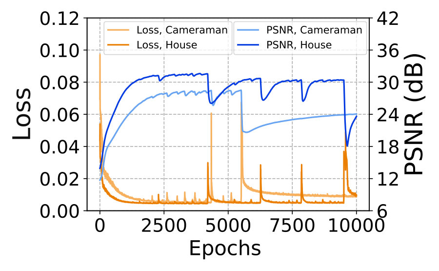 Figure 1
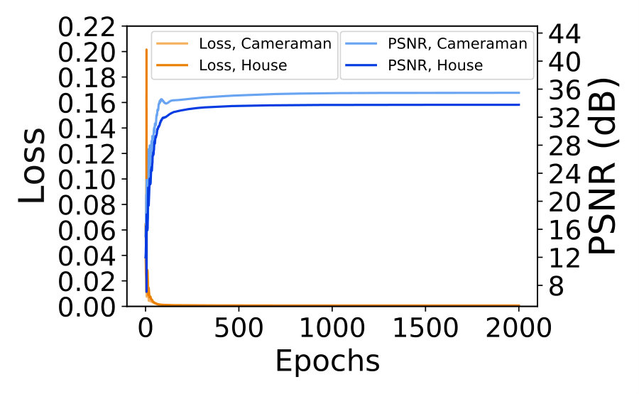 Figure 2
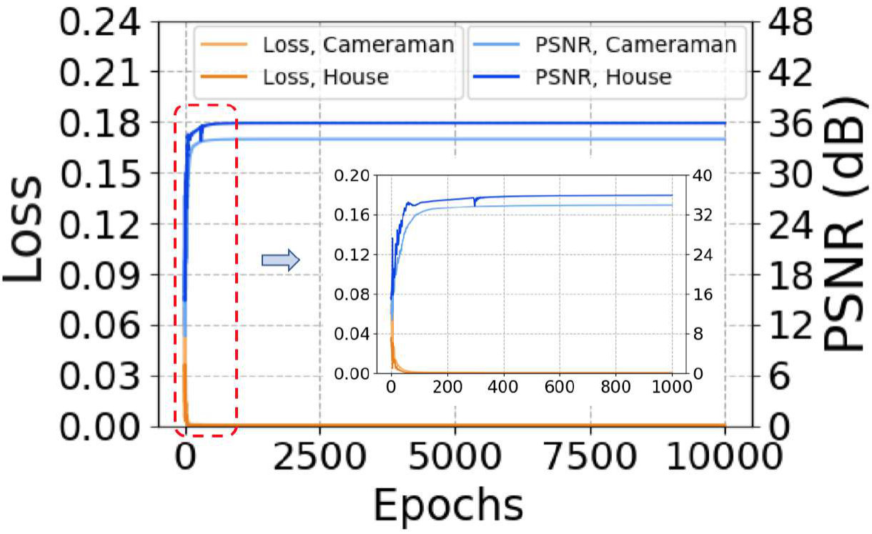 Figure 3
 Figure 4
 Figure 5
 Figure 6
 Figure 7
 Figure 8
 Figure 9
 Figure 10
 Figure 11
 Figure 12
 Figure 13
 Figure 14
 Figure 15
 Figure 16
 Figure 17
 Figure 18
 Figure 19
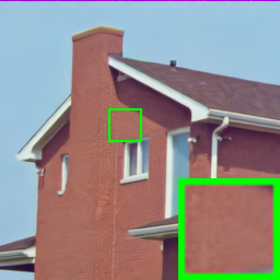 Figure 20
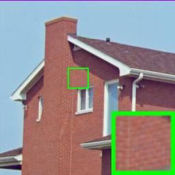 Figure 21
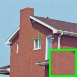 Figure 22
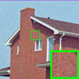 Figure 23
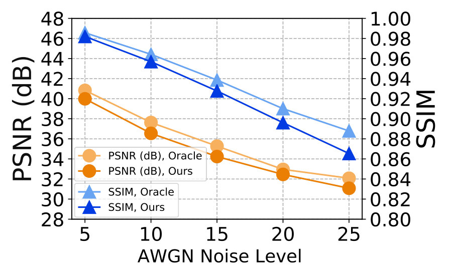 Figure 24
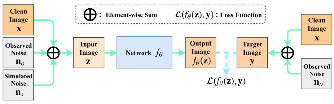 Figure 25
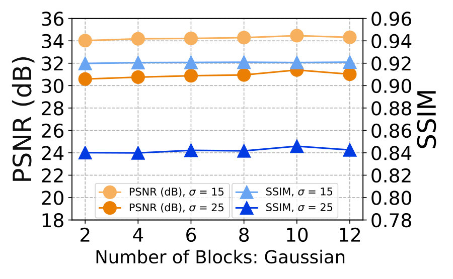 Figure 26
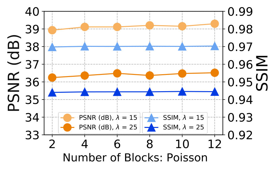 Figure 27
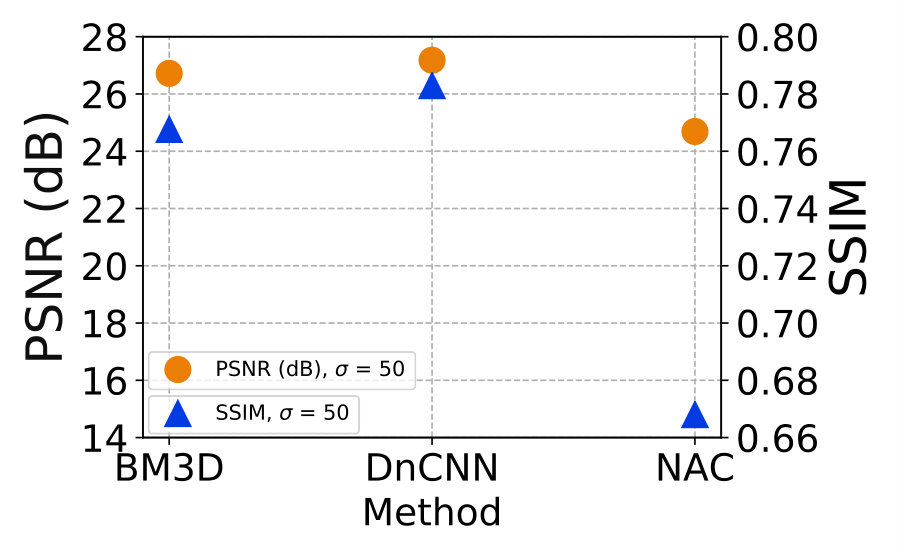 Figure 28
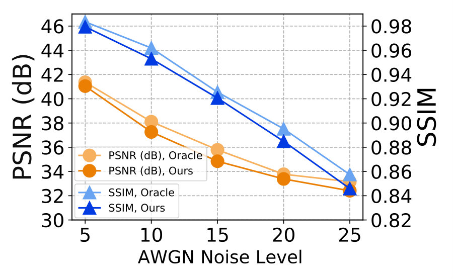 Figure 29
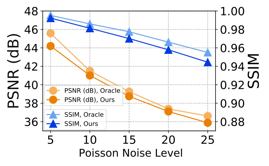 Figure 30
 Figure 31
 Figure 32
 Figure 33
 Figure 34
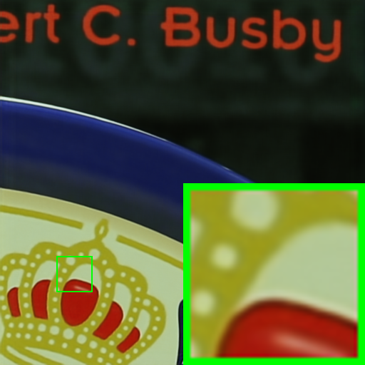 Figure 35
 Figure 36
 Figure 37
 Figure 38
 Figure 39
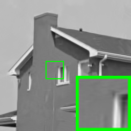 Figure 40
| Image | Noise | |||
| Type | Method | Year’Pub. | Prior | Stat. |
| S. | DnCNN [41] | 17’TIP | Ext. | ✓ |
| CBDNet [14] | 19’CVPR | Ext. | ✓ | |
| U. | Noise2Noise [22] | 18’ICML | Ext. | ✓ |
| GAN-CNN [7] | 18’CVPR | Ext. | ✓ | |
| Noise2Void [19] | 19’CVPR | Ext. | ||
| SS. | Deep Image Prior [23] | 18’CVPR | Int. | |
| Noise2Self [3] | 19’ICML | Ext. | ||
| Self-Supervised [20] | 19’NeurIPS | Ext. | ||
| Noisy-As-Clean (Ours) | 20’Submit | Int. | ✓ |
| Noise Level | |||||||||||||||
| Metric | PSNR | SSIM | PSNR | SSIM | PSNR | SSIM | PSNR | SSIM | PSNR | SSIM | |||||
| BM3D [10] | 38.07 | 0.9580 | 34.40 | 0.9234 | 32.38 | 0.8957 | 31.00 | 0.8717 | 29.97 | 0.8503 | |||||
| DnCNN [41] | 38.76 | 0.9633 | 34.78 | 0.9270 | 32.86 | 0.9027 | 31.45 | 0.8799 | 30.43 | 0.8617 | |||||
| N2N [22] | 39.72 | 0.9665 | 36.18 | 0.9446 | 33.99 | 0.9149 | 32.10 | 0.8788 | 30.72 | 0.8446 | |||||
| DIP [23] | 32.49 | 0.9344 | 31.49 | 0.9299 | 29.59 | 0.8636 | 27.67 | 0.8531 | 25.82 | 0.7723 | |||||
| N2V [19] | 27.06 | 0.8174 | 26.79 | 0.7859 | 26.12 | 0.7468 | 25.89 | 0.7405 | 25.01 | 0.6564 | |||||
| DnCNN+NAC | 43.17 | 0.9817 | 37.16 | 0.9336 | 33.64 | 0.8697 | 31.15 | 0.8024 | 29.22 | 0.7382 | |||||
| Blind DnCNN+NAC | 43.16 | 0.9817 | 37.14 | 0.9333 | 33.63 | 0.8693 | 31.14 | 0.8018 | 29.21 | 0.7376 | |||||
| ResNet+NAC | 39.99 | 0.9820 | 36.55 | 0.9569 | 34.24 | 0.9277 | 32.46 | 0.8961 | 31.08 | 0.8654 | |||||
| Blind ResNet+NAC | 38.48 | 0.9805 | 36.65 | 0.9564 | 34.77 | 0.9275 | 33.13 | 0.9024 | 31.78 | 0.8802 | |||||
| Noise Level | |||||||||||||||
| Metric | PSNR | SSIM | PSNR | SSIM | PSNR | SSIM | PSNR | SSIM | PSNR | SSIM | |||||
| BM3D [10] | 37.59 | 0.9640 | 33.32 | 0.9163 | 31.07 | 0.8720 | 29.62 | 0.8342 | 28.57 | 0.8017 | |||||
| DnCNN [41] | 38.07 | 0.9695 | 33.88 | 0.9270 | 31.73 | 0.8706 | 30.27 | 0.8563 | 29.23 | 0.8278 | |||||
| N2N [22] | 38.58 | 0.9627 | 34.07 | 0.9200 | 31.81 | 0.8770 | 30.14 | 0.8550 | 28.67 | 0.8123 | |||||
| DIP [23] | 29.74 | 0.8435 | 28.16 | 0.8310 | 27.07 | 0.7867 | 25.80 | 0.7205 | 24.63 | 0.6680 | |||||
| N2V [19] | 26.70 | 0.7915 | 26.39 | 0.7621 | 25.77 | 0.7126 | 25.41 | 0.6678 | 24.83 | 0.6305 | |||||
| DnCNN+NAC | 40.21 | 0.9674 | 34.21 | 0.8913 | 30.72 | 0.8044 | 28.25 | 0.7230 | 26.34 | 0.6515 | |||||
| Blind DnCNN+NAC | 40.20 | 0.9674 | 34.21 | 0.8911 | 30.71 | 0.8041 | 28.24 | 0.7227 | 26.33 | 0.6511 | |||||
| ResNet+NAC | 39.00 | 0.9707 | 34.60 | 0.9324 | 32.13 | 0.8942 | 30.47 | 0.8636 | 28.96 | 0.8185 | |||||
| Blind ResNet+NAC | 38.26 | 0.9605 | 34.26 | 0.9266 | 32.06 | 0.8919 | 30.50 | 0.8609 | 29.33 | 0.8327 | |||||
| Type | Traditional Methods | Supervised Networks | Unsupervised Networks | Self-supervised Networks | |||||
| Dataset | Method | CBM3D [9] | NI [2] | DnCNN+[41] | CBDNet [14] | GCBD [7] | N2N [22] | DIP [23] | Blind ResNet+NAC |
| CC [28] | PSNR | 35.19 | 35.33 | 35.40 | 36.44 | NA | 35.32 | 35.69 | 36.59 |
| SSIM | 0.9063 | 0.9212 | 0.9115 | 0.9460 | NA | 0.9160 | 0.9259 | 0.9502 | |
| DND [29] | PSNR | 34.51 | 35.11 | 37.90 | 38.06 | 35.58 | 33.10 | NA | 36.20 |
| SSIM | 0.8507 | 0.8778 | 0.9430 | 0.9421 | 0.9217 | 0.8110 | NA | 0.9252 | |
| # of Blocks | 1 | 2 | 5 | 10 | 15 |
| PSNR | 33.58 | 33.85 | 34.14 | 34.24 | 34.26 |
| SSIM | 0.9161 | 0.9226 | 0.9272 | 0.9277 | 0.9272 |
| # of Epochs | 100 | 200 | 500 | 1000 | 5000 |
| PSNR | 31.80 | 32.79 | 33.77 | 34.24 | 34.28 |
| SSIM | 0.8714 | 0.9023 | 0.9189 | 0.9277 | 0.9280 |
| Time | 67.4 | 132.5 | 302.0 | 583.2 | 2815.6 |
Peer Reviews
No public reviews on file for this paper yet. If you reviewed it on a platform where reviews are public (OpenReview, ICLR, NeurIPS, ICML), you can paste yours below so the community can read it here.
Code & Models
Videos
No videos yet. Explain this paper in a talk, walkthrough, or lecture? Add one.
Taxonomy
MethodsAverage Pooling · *Communicated@Fast*How Do I Communicate to Expedia? · 1x1 Convolution · Batch Normalization · Bottleneck Residual Block · Global Average Pooling · Residual Block · Kaiming Initialization · Max Pooling · Residual Connection
Noisy-As-Clean: Learning Self-supervised Denoising from the Corrupted Image
Jun Xu, Yuan Huang, Ming-Ming Cheng, Li Liu, Fan Zhu, Zhou Xu, Ling Shao
This work was supported in part by the Major Project for New Generation of AI under Grant No. 2018AAA0100400, NSFC (61922046), and Tianjin Natural Science Foundation (18ZXZNGX00110). (∗Corresponding author: M.-M. Cheng)
J. Xu and M.-M. Cheng are with TKLNDST, College of Computer Science, Nankai University, Tianjin, China (E-mail: [email protected], [email protected]). Y. Huang is with School of Electronic and Information Engineering, Xi’an Jiaotong University, Xi’an, China. L. Liu, F. Zhu, and L. Shao are with Inception Institute of Artificial Intelligence (IIAI) and Mohamed bin Zayed University of Artificial Intelligence (MBZUAI), Abu Dhabi, UAE. Zhou Xu is with School of Big Data and Software Engineering, Chongqing University, Chongqing, China. The first two authors contribute equally.
Abstract
Supervised deep networks have achieved promising performance on image denoising, by learning image priors and noise statistics on plenty pairs of noisy and clean images. Unsupervised denoising networks are trained with only noisy images. However, for an unseen corrupted image, both supervised and unsupervised networks ignore either its particular image prior, the noise statistics, or both. That is, the networks learned from external images inherently suffer from a domain gap problem: the image priors and noise statistics are very different between the training and test images. This problem becomes more clear when dealing with the signal dependent realistic noise. To circumvent this problem, in this work, we propose a novel “Noisy-As-Clean” (NAC) strategy of training self-supervised denoising networks. Specifically, the corrupted test image is directly taken as the “clean” target, while the inputs are synthetic images consisted of this corrupted image and a second and similar corruption. A simple but useful observation on our NAC is: as long as the noise is weak, it is feasible to learn an self-supervised network only with the corrupted image, approximating the optimal parameters of a supervised network learned with pairs of noisy and clean images. Experiments on synthetic and realistic noise removal demonstrate that, the DnCNN and ResNet networks trained with our self-supervised NAC strategy achieve comparable or better performance than the original ones and previous supervised/unsupervised/self-supervised networks. The code is publicly available at https://github.com/csjunxu/Noisy-As-Clean.
Index Terms:
Image denoising, self-supervision, convolutional neural network.
I Introduction
Image denoising is an ill-posed inverse problem to recover a clean image from the observed noisy image , where is the observed corrupted noise. One popular assumption on is the additive white Gaussian noise (AWGN) with standard deviation (std) , which serves as a perfect test bed for supervised networks in the deep learning era [32, 33, 15]. Supervised networks [21, 41, 30] learn the image priors and noise statistics on plenty pairs of clean and corrupted images, and achieve promising denoising performance on the images with similar priors and noise statistics (e.g., AWGN).
With advances on AWGN noise removal [6, 41, 30], a natural question arises is how these denoising networks can exert their effect on real noisy photographs. Realistic noise is signal dependent and more complex than AWGN [28, 29, 36]. Thus, previous supervised denoising networks unavoidably suffer from a domain gap problem: both the image priors and noise statistics in training are different from those of the real-world test images. Recently, several unsupervised [7, 22, 23, 19] and self-supervised [3, 20] networks have been developed to get rid of the dependence on clean images, which are difficult to be obtained in real-world scenarios. However, unsupervised networks are subjected to the gap on either image priors or noise statistics, while self-supervised suffer from the gap on noise statistics, between the external images for training and the corrupted ones for test. Besides, several networks [22, 23] succeed on the zero-mean noise. But the realistic noise in real-world images is not necessarily zero-mean [28, 29, 1].
To alleviate the domain gap on image priors and noise statistics between training and test images, in this paper, we propose a “Noisy-As-Clean” (NAC) strategy for training self-supervised denoising networks. In our NAC, we directly train an image-specific network by taking the corrupted image as the “clean” target. Thus, the domain gap on image priors are largely bridged by our NAC. To reduce the gap on noise statistics, for the target corrupted image , we take as the input of our NAC a simulated noisy image consisting of the corrupted image and a simulated noise , which is statistically close to the corrupted noise in . By this way, our NAC network learns to clean up the simulated noise from the doubly corrupted image during training, and thus is able to remove the noise from the corrupted image during test.
A simple but useful observation about our NAC strategy is: as long as the corrupted noise is “weak”, it is feasible to train a self-supervised denoising network only with the corrupted test image, and the learned parameters are very close to those of a supervised network trained with a pair of the corrupted image and its clean version. Though being very simple, our NAC strategy is very effective for image denoising. In Figure 1, we compare the denoised images by the vanilla DnCNN [41] and the DnCNN trained with our NAC (DnCNN+NAC), on the image “House” corrupted by AWGN (). We observe that the “DnCNN+NAC” achieves better visual quality and higher PSNR/SSIM results than DnCNN [41], which is trained on plenty of noisy and clean image pairs. Experiments on diverse benchmarks demonstrate that, when trained with our NAC strategy, the DnCNN [41] and ResNet [15] in Deep Image Prior (DIP) [23] achieve comparable or better performance than supervised denoising networks on synthetic and real-world noisy images. Our work reveals that, when the noise is “weak”, a self-supervised network trained directly on the corrupted image can obtain comparable or even better performance than supervised networks on image denoising.
In summary, our contribution are mainly three-fold:
- •
We propose a “Noisy-As-Clean” (NAC) strategy for training self-supervised denoising networks.
- •
We provide a theoretical background of our NAC strategy, and implement the DnCNN [41] and ResNet in DIP [23] into self-supervised networks by our NAC for effective image denoising.
- •
Experiments on synthetic and real-world benchmarks show that, on weak noise, the DnCNN and ResNet in [23] trained by our NAC achieve comparable or even better performance than the comparison denoising networks.
The remaining parts of this paper are organized as follows. In §II, we introduce the related work. In §III, we present the theoretical background of our NAC strategy for self-supervised image denoising. In §IV, we implement the DnCNN [41] and ResNet used in [23] as self-supervised networks by our NAC. Extensive experiments are conducted in §V demonstrate that, the DnCNN and ResNet networks trained by our NAC achieve comparable or even better performance than previous supervised image denoising networks on benchmark synthetic and real-world datasets. Conclusion is given in §VI.
II Related Work
In Table I, we summarize several state-of-the-art supervised [41, 14], unsupervised [22, 7, 19] and self-supervised [23, 3, 20] networks, image priors, and noise statistics. In this work, to bridge the domain gap problem, we propose a “Noisy-As-Clean” strategy to learn the image-specific internal prior and noise statistics directly from the corrupted test image.
Supervised denoising networks are trained with plenty pairs of noisy and clean images. This category of networks can learn external image priors and noise statistics from the training data. Several methods [41, 30, 26] have been developed with achieving promising performance on AWGN noise removal, where the statistics of training and test noise are similar. However, due to the aforementioned domain gap problem, the performance of these networks degrade severely on real-world noisy images [28, 29, 36].
Unsupervised and self-supervised denoising networks are developed to remove the need on plenty of clean images. Along this direction, Noise2Noise (N2N) [22] trains the network between pairs of corrupted images with the same scene, but independently sampled noise. This work is feasible to learn external image priors and noise statistics from the training data. However, in real-world scenarios, it is difficult to collect large amounts of paired images with independent corruption for training. Noise2Void (N2V) [19] predicts a pixel from its surroundings by learning blind-spot networks, but it still suffers from the domain gap on image priors between the training images and test images. This work assumes that the corruption is zero-mean and independent between pixels. However, as mentioned in Noise2Self (N2S) [3], N2V [19] significantly degrades the training efficiency and denoising performance at test time. Recently, Deep Image Prior (DIP) [23] reveals that the network structure can resonate with the natural image priors, and can be utilized in image restoration without external images. However, it is not practical to select a suitable network and early-stop its training at right moments for each corrupted image. Self-supervised denoisers [3, 20] employ explicit corruption models, and train the networks only with the corrupted image itself. In this work, we utilize the helpful noise model to learn self-supervised denoising networks for real-world image denoising.
Internal and external image priors are widely used for diverse image restoration tasks [39, 31, 40]. Internal priors are directly learned from the input test image itself, such as the multi-scale priors [12, 35, 11], image-specific details [42, 24], and non-local self similarity [39, 38, 16]. The external ones are learned on external natural images [43, 40, 37]. Internal priors are adaptive to its image contents, but somewhat affected by the corruptions [12, 42]. By contrast, the external priors are effective for restoring images with general contents, but may not be optimal for specific test image [43, 40, 8].
Noise statistics is of key importance for image denoising. The AWGN noise is one typical noise with widespread study. Recently, researchers shift more attention to the realistic noise produced in camera sensors [29, 1], which is usually modeled as mixed Poisson and Gaussian distribution [13]. The Poisson component mainly comes from the irregular photons hitting the sensor [25], while Gaussian noise is majorly produced by dark current [28]. Though performing well on the synthetic noise being trained with, supervised denoisers [41, 26, 14] still suffer from the domain gap problem when processing the real-world noisy images.
III Theoretical Background of “Noisy-As-Clean”
Training a supervised network (parameterized by ) requires many pairs of noisy image and clean image , by minimizing an empirical loss function as
[TABLE]
Assuming that the probability of occurrence for pair is , then statistically we have
[TABLE]
where and are random variables of noisy and clean images, respectively. The paired variables are dependent, and their relationship is , where is the random variable of observed noise. By exploring the dependence of , Eqn. (2) is equivalent to
[TABLE]
This indicates that the network can minimize the loss function by solving Eqn. (3) separately for each clean image.
Different with the “zero-mean” assumption in [22, 19], here we study a more practical assumption on noise statistics, i.e., the expectation and variance of signal intensity are much stronger than those of noise and (negligible but not necessarily zero):
[TABLE]
This is actually valid in real-world scenarios, since we can clearly observe the contents in most real photographs, with little influence of the noise. The noise therein is often modeled by zero-mean Gaussian or mixed Poisson and Gaussian (for realistic noise). Hence, the noisy image should have similar expectation with the clean image :
[TABLE]
Now we add simulated noise to the observed noisy image , and generate a new noisy image . We assume that is statisticly close to , i.e., and . Then we have
[TABLE]
Therefore, the simulated noisy image has similar expectation with the observed noisy image :
[TABLE]
By the Law of Total Expectation [4], we have
[TABLE]
Since the loss function (usually ) and the conditional probability density functions and are all continuous everywhere, the optimal network parameters of Eqn. (3) changes little with the addition of negligible noise or . With Eqns. (4)-(8), when the -conditioned expectation of are replaced with the -conditioned expectation of , obtains similar -conditioned optimal parameters :
[TABLE]
The network minimizes the loss function for each input image pair separately, which equals to minimize it on all finite pairs of images. Through simple manipulations, Eqn. (9) is equivalent to
[TABLE]
By exploring the dependence of , Eqn. (10) is equivalent to
[TABLE]
A simple but useful observation is: as long as the noise is weak, the optimal parameters of self-supervised network trained on noisy image pairs are very close to the optimal parameters of the supervised networks trained on pairs of noisy and clean images . In Figure 3, we explain our NAC strategy and illustrate this observation through an example on the image “Test004” from the BSD68 dataset: The clean image in (a) is firstly corrupted by observed AWGN noise with . Then we add simulated AWGN noise also with to the corrupted image in (b), and obtain a doubly corrupted image in (c). The DnCNN [41] with our NAC strategy, named as DnCNN+NAC, is trained with the doubly corrupted image in (c) as input and the corrupted image in (b) as target. The final training output is plotted in (d), with similar PSNR and SSIM [34] results as the corrupted image in (b). Then the DnCNN+NAC network learned on (b) and (c) is directly employed to perform inference on the corrupted image in (b), and produces the testing output in (e). When compared to DnCNN [41], our DnCNN+NAC achieves much higher PSNR and SSIM results on the corrupted image (b). The estimated simulated noise and observed noise in training and test stages are plotted in (g) and (h), respectively. One can see that they are visually in similar noise statistics.
Consistency of noise statistics. Since our contexts are the real-world scenarios, the noise can be modeled by mixed Poisson and Gaussian distribution [13]. Fortunately, both the two distributions are linear additive, i.e., the addition variable of two Poisson (or Gaussian) distributed variables are still Poisson (or Gaussian) distributed. Assume that the observed (simulated) noise () follows a mixed -dependent (-dependent) Poisson distribution parameterized by () and Gaussian distribution (), i.e.,
[TABLE]
where and indicates that the noise and are element-wisely dependent on and , respectively. The “” is valid if we assume that the observed noise is “weak” when compared to the signal . To this end, we have
[TABLE]
where is the correlation between and ( if they are independent). This indicates that the summed noise variable still follows a mixed dependent Poisson and Gaussian distribution, guaranteeing the consistency in noise statistics between the observed realistic noise and the simulated noise. As will be validated by the experiments (§V), this property makes our NAC strategy consistently effective on different noise removal tasks.
IV Learning Self-supervised Denoising Networks
by “Noisy-As-Clean”
Here, we propose to learn self-supervised denoising networks with our “Noisy-As-Clean” (NAC) strategy. We employ the DnCNN [41] and ResNet in DIP [23] as our baseline, and call the self-supervised networks as DnCNN+NAC and ResNet+NAC, respectively. Note that we only need the observed noisy image to generate noisy image pairs with simulated noise , as illustrated in Figure 2.
Training self-supervised networks by our NAC. For real-world images captured by camera sensors, one can hardly distinguish the realistic noise from the signal. The signal intensity is usually stronger than the noise intensity. That is, the expectation of the observed realistic noise is usually much smaller than that of the latent clean image . If we train an image-specific network for the new noisy image and regard the original noisy image as the ground-truth image, then the trained image-specific network basically joint learn the image-specific prior and noise statistics. It has the capacity to remove the noise from the new noisy image . Then if we perform denoising on the original noisy image , the observed noise can be well-removed. Note that we do not use the clean image as “ground-truth” in training the DnCNN+NAC and ResNet+NAC networks.
Training blind denoising networks. Most of existing supervised denoising networks train a specific model to process a fixed noise pattern [28, 26, 5]. To tackle unknown noise, one feasible solution for these networks is to assume the noise as AWGN and estimate its noise deviation. The corresponding noise is removed by using the networks trained with the estimated level. But this strategy largely degrades the denoising performance when the noise deviation is not estimated accurately. Besides, this solution can hardly deal with realistic noise, which is usually not AWGN, captured on real photographs. In order to be effective on removing realistic noise, the self-supervised networks by our NAC are feasible to blindly remove the unknown noise from real photographs. Inspired by [41, 14], we propose to train a blind version of DnCNN+NAC and ResNet+NAC networks by using the AWGN noise within a range of levels (e.g., ) for removing unknown AWGN noise. We also train blind ResNet+NAC with mixed AWGN and Poisson noise (both within a range of intensities) for removing the realistic noise. More details will be explained in §V-B.
Testing is performed by directly regarding an observed noisy image as input. We only test the image once. The denoised image can be represented as , with which the objective metrics, e.g., PSNR and SSIM [34], can be computed with the clean image .
Implementation details. We employ the DnCNN [41] and ResNet in DIP [23] as the backbones, and turn them into self-supervised networks by our NAC strategy, which are named as DnCNN+NAC and ResNet+NAC, respectively. The DnCNN contains 17 layers of convolution, Batch Normalization (BN) [17], and Rectified Linear Units (ReLU) activation operator [27]. To accommodate DnCNN with our NAC strategy, we set the output of DnCNN+NAC as the denoised image, not the residual noise in DnCNN [41]. We observe no difference between the results on PSNR, SSIM [34], and visual quality by employing these two types of outputs in our experiments. As DnCNN, the parameters of DnCNN+NAC are initialized from a pretrained ResNet. As used in [23], the ResNet in our ResNet+NAC includes residual blocks, each containing two convolutional layers followed by a BN [17] and a ReLU [27] after the first BN. The parameters are randomly initialized without being pretrained. For both baselines, the optimizer is Adam [18] with default parameters. The learning rate is fixed at in all experiments. We use the loss function. For each test image, we only train the DnCNN+NAC in 100 epochs, while the original DnCNN is trained with 180 epochs. The ResNet+NAC is trained in epochs for each test image, the same as that in DIP [23]. As suggested by DnCNN [41] and DIP [23], we employ rotations {0°, 90°, 180°, 270°} combined with 2 mirror (vertical and horizontal) reflections, resulting in totally transformations for data augmentation. We implement the DnCNN+NAC and ResNet+NAC networks in PyTorch.
V Experiments
In this section, we evaluate the performance of our “Noisy-As-Clean” (NAC) networks on image denoising. In all experiments, we train a denoising network using only the noisy test image as the target, and using the simulated noisy image as the input. For all comparison methods, the source codes or trained models are downloaded from the corresponding authors’ websites. We use the default parameter settings, unless otherwise specified. The PSNR, SSIM [34], and visual quality of different methods are used to evaluate the comparison. We first test with synthetic noise such as additive white Gaussian noise (AWGN) in §V-A, continue to perform blind image denoising in §V-B, and finally tackle the realistic noise in §V-C. In §V-D, we conduct comprehensive ablation studies to gain deeper insights into our NAC strategy.
V-A Synthetic Noise Removal With Known Noise
We evaluate the DnCNN+NAC and ResNet+NAC networks on images corrupted by synthetic AWGN noise. More results on signal dependent Poisson noise and mixed Poisson-AWGN noise are provided in the Supplementary File.
Training self-supervised networks. Here, we train an image-specific denoising network using the observed noisy test image as the target, and the simulated noisy image as the input. Each observed noisy image is generated by adding the observed noise to the clean image . The simulated noisy image is generated by adding simulated noise to observed noisy image .
Comparison methods. We compare DnCNN+NAC and ResNet+NAC networks with state-of-the-art image denoising methods [10, 41, 22]. On AWGN noise, we compare with BM3D [10], DnCNN [41], Noise2Noise (N2N) [22], Deep Image Prior (DIP) [23], and Noise2Void (N2V) [19].
Test datasets. We evaluate the comparison methods on the Set12 and BSD68 datasets, which are widely tested by supervised denoising networks [41, 26] and previous methods [10, 40]. The Set12 dataset contains 12 images of sizes or , while the BSD68 dataset contains 68 images of different sizes.
Results on AWGN noise with noise levels (standard deviation, or std) of are provided here. The observed noise is AWGN with std of , while the simulated noise is with the same as that of . The comparison results are listed in Tables II and III. It can be seen that, DnCNN+NAC achieves better PSNR and SSIM results than those of the original DnCNN when . Note that DnCNN are supervised networks trained offline on the BSD400 dataset, while the variant DnCNN+NAC network is trained online for each corrupted image. Besides, the blind version of DnCNN+NAC achieves negligible performance drop when compared to the DnCNN+NAC, which is consistent with [41]. On the other side, the ResNet+NAC networks achieve comparable or better performance on PSNR and SSIM [34] than BM3D [10] and DnCNN [41], especially when the noise levels are weak (). Besides, our ResNet+NAC networks outperform the other unsupervised and self-supervised networks such as N2N [22], DIP [23], and N2V [19] by a large margin on PSNR and SSIM [34]. In Figures 4 and 5, we provide the visual comparisons of the denoised images by the competing methods. One can see that the ResNet+NAC networks produce better image quality and higher PSNR/SSIM results than the comparison methods.
V-B Synthetic Noise Removal With Unknown Noise
To deal with unknown noise, we propose to train blind versions of the DnCNN [41] and ResNet in [23] by our NAC strategy. Here, we test the Blind DnCNN+NAC and Blind ResNet+NAC networks on AWGN noise with unknown noise deviation. We use the same training strategy, comparison methods, and test datasets as in §V-A.
Training blind networks. We train the Blind DnCNN+NAC and Blind ResNet+NAC networks on the corrupted test image degraded again by AWGN noise with unknown noise levels (deviations). The noise levels are randomly sampled in Gaussian distribution within . We also test on noise levels in uniform distribution and obtain similar results. We repeat the training of DnCNN+NAC and ResNet+NAC networks on the test image with different deviations.
Results on blind denoising. For the same test image, we add to it the AWGN noise whose deviation is also in . The blindly trained DnCNN+NAC and ResNet+NAC networks are directly utilized to denoise the test image without estimating its deviation. The results are also listed in Tables II and III. We observe that, the Blind ResNet+NAC networks trained on AWGN noise with unknown levels can achieve even better PSNR and SSIM [34] results than the ResNet+NAC networks trained on specific noise levels. Note that on BSD68, the ResNet+NAC networks achieve higher PSNR and SSIM results than DnCNN [41]. This demonstrates the effectiveness of our ResNet+NAC networks on blind image denoising. With the success on blind image, next we will turn to real-world image denoising, in which the noise is also unknown and very complex.
V-C Practice on Real Photographs
With the promising performance on blind image denoising, here we tackle the realistic noise for practical applications. The observed realistic noise can be roughly modeled as mixed Poisson noise and AWGN noise [13, 14]. Hence, for each observed noisy image , we generate the simulated noise by sampling the -dependent Poisson part and the independent AWGN noise.
Training blind ResNet+NAC networks is also performed for each test image, i.e., the observed noisy image . In real-world scenarios, each observed noisy image is corrupted without knowing the specific noise statistics of the observed noise . Therefore, the simulated noise is directly estimated on as mixed -dependent Poisson and AWGN noise. For each transformation image in data augmentation, the Poisson noise is randomly sampled with the parameter in , and the AWGN noise is randomly sampled with the noise level in .
Comparison methods. We compare with state-of-the-art methods on real-world image denoising, including CBM3D [9], the commercial software Neat Image [2], two supervised networks DnCNN+ [41] and CBDNet [14], and two unsupervised networks GCBD [7] and Noise2Noise [22], and the self-supervised network DIP [23]. Note that DnCNN+ [41] and CBDNet [14] are two state-of-the-art supervised networks for real-world image denoising, and DnCNN+ is an improved extension of DnCNN [41] with better performance (the authors of DnCNN+ provide us the models/results of DnCNN+).
Test datasets. We evaluate the comparison methods on the Cross-Channel (CC) dataset [28] and DND dataset [29]. The CC dataset [28] includes noisy images of 11 static scenes captured by Canon 5D Mark 3, Nikon D600, and Nikon D800 cameras. The noisy images are collected under a highly controlled indoor environment. Each scene is shot times using the same settings. The average of the shots is taken as “ground-truth”. We use the default images of size cropped by the authors to evaluate different image denoising methods. The DND dataset [29] contains 50 scenarios captured by Sony A7R, Olympus E-M10, Sony RX100 IV, and Huawei Nexus 6P. Each scene is cropped to 20 bounding boxes of pixels, generating totally 1000 test images. The noisy images are collected under higher ISO values with shorter exposure times, while the “ground truth” images are captured under lower ISO values with adjusted longer exposure times. The “ground truth” images are not released, but we can obtain the PSNR and SSIM results by submitting the denoised images to the DND’s Website.
Comparison results on PSNR and SSIM are listed in Table IV. As can be seen, the ResNet+NAC networks achieve better performance than all previous denoising methods, including the CBM3D [9], the supervised networks DnCNN+ [41] and CBDNet [14], and the unsupervised networks GCBD [7], N2N [22], and DIP [23]. This demonstrates that the ResNet+NAC networks can indeed handle the complex, unknown, and realistic noise, and achieve better performance than supervised networks such as DnCNN+ [41] and CBDNet [14].
Qualitative results. In Figures 6 and 7, we show the denoised images of our ResNet+NAC and the comparison methods on the images of “5dmark3-iso3200-1” from the CC dataset [28] and “0017_3” from the DND dataset [29], respectively. We observe that our self-supervised Blind ResNet+NAC is very effective on removing realistic noise from the real photograph. Besides, the Blind ResNet+NAC networks achieve competitive PSNR and SSIM results when compared with the other methods, including the supervised DnCNN+ [41] and CBDNet [14].
Speed. The work most similar to ours is Deep Image Prior (DIP) [23], which also trains an image-specific network for each test image. Averagely, DIP needs seconds to process a color image, on which our ResNet+NAC network needs seconds (on an NVIDIA Titan X GPU).
V-D Ablation Study
To further study our NAC strategy, we conduct more examination of our ResNet+NAC networks on image denoising. Specifically, we assess 1) differences of the ResNet+NAC from the ResNet in DIP [23]; 2) how the number of residual blocks and epochs influence the ResNet+NAC; 3) comparison with the “Oracle” performance of the ResNet+NAC networks; 4) performance of the ResNet+NAC on “strong” noise.
1) Differences from DIP [23]. Though the basic network in our work is the ResNet used in DIP [23], our ResNet+NAC network is essentially different from DIP on at least two aspects. First, our ResNet+NAC is a novel strategy for self-supervised learning of adaptive network parameters for the degraded image, while DIP aims to investigate adaptive network structure without learning the parameters. Second, our ResNet+NAC learns a mapping from the synthetic noisy image to the noisy image , which approximates the mapping from the noisy image to the clean image . But DIP maps a random noise map to the noisy image , and the denoised image is obtained during the process. Due to the two reasons, DIP needs early stop for different images, while our ResNet+NAC achieves more robust (and better) denoising performance than DIP on diverse images. In Figure 8, we plot the curves of training loss and test PSNR of DIP (a) and ResNet+NAC (b) networks in 10,000 epochs, on two images of “Cameraman” and “House”. We observe that DIP needs early stop to select the best results, while our ResNet+NAC can stably achieve better denoising results within 1000 epochs.
2) Influence on the number of residual blocks and epochs. Our backbone network is the ResNet [23] with 10 residual blocks trained in 1000 epochs. Now we study how the number of residual blocks and epochs influence the performance of ResNet+NAC on image denoising. The experiments are performed on the Set12 dataset corrupted by AWGN noise (). From Table V, we observe that, with more residual blocks, the ResNet+NAC networks can achieve better PSNR and SSIM [34] results. And 10 residual blocks are enough to achieve satisfactory results. With more (e.g., 15) blocks, there is little improvement on PSRN and SSIM. Hence, we use 10 residual blocks the same as [23]. Then we study how the number of epochs influence the performance of ResNet+NAC on image denoising. From Table VI, one can see that on the Set12 dataset corrupted by AWGN noise (), with more training epochs, our ResNet+NAC networks achieve better PSNR and SSIM results, but with longer processing time.
3) Comparison with Oracle. We also study the “Oracle” performance of the ResNet+NAC networks. In “Oracle”, we train the ResNet+NAC networks on the pair of observed noisy image and its clean image corrupted by AWGN noise or signal dependent Poisson noise. The experiments are performed on Set12 dataset corrupted by AWGN or signal dependent Poisson noise. The noise deviations are in . Figure 9 (a) shows comparisons of our ResNet+NAC and its “Oracle” networks on PSNR and SSIM. It can be seen that, the “Oracle” networks trained on the pair of noisy-clean images only perform slightly better than the original ResNet+NAC networks trained with the simulated-observed noisy image pairs . With our NAC strategy, the ResNet networks trained only with noisy test images achieves similar promising performance on the weak noise.
4) Performance on strong noise. Our NAC strategy is based on the assumption of “weak noise”. It is natural to wonder how well ResNet+NAC performs against strong noise. To answer this question, we compare the ResNet+NAC networks with BM3D [10] and DnCNN [41], on Set12 corrupted by AWGN noise with . The PSNR and SSIM results are plotted in Figure 9 (b). One can see that, our ResNet+NAC networks are limited in handling strong AWGN noise, when compared with BM3D [10] and DnCNN [41].
VI Conclusion
In this work, we proposed a “Noisy-As-Clean” (NAC) strategy for learning self-supervised image denoising networks. In our NAC, we trained an image-specific network by taking the corrupted image as the target, and adding to it the simulated noise to generate the doubly corrupted noisy input. The simulated noise is close to the observed noise in the noisy test image. This strategy can be seamlessly embedded into existing supervised denoising networks. We observed that it is possible to learn a self-supervised network only with the corrupted image, approximating the optimal parameters of a supervised network learned with a pair of noisy and clean images. Extensive experiments on synthetic and real-world benchmarks demonstrate that, the DnCNN [41] and ResNet in Deep Image Prior [23] trained with our NAC strategy achieved comparable or better performance on PSNR, SSIM, and visual quality, when compared to previous state-of-the-art image denoising methods, including supervised denoising networks. These results validate that our NAC strategy can learn effctive image-specific priors and noise statistics only from the corrupted test image.
The reference list from the paper itself. Each links out to its DOI / PubMed record.
- 1[1] A. Abdelhamed, S. Lin, and M. S. Brown. A high-quality denoising dataset for smartphone cameras. In CVPR , June 2018.
- 2[2] N. AB Soft. Neat Image. https://ni.neatvideo.com/home .
- 3[3] J. Batson and L. Royer. Noise 2Self: Blind denoising by self-supervision. In ICML , volume 97, pages 524–533. PMLR, 2019.
- 4[4] P. Billingsley. Probability and Measure . Wiley Series in Probability and Statistics. Wiley, 1995.
- 5[5] T. Brooks, B. Mildenhall, T. Xue, J. Chen, D. Sharlet, and J. T. Barron. Unprocessing images for learned raw denoising. In CVPR , pages 9446–9454, 2019.
- 6[6] H. C. Burger, C. J. Schuler, and S. Harmeling. Image denoising: Can plain neural networks compete with BM 3D? In CVPR , pages 2392–2399, 2012.
- 7[7] J. Chen, J. Chen, H. Chao, and M. Yang. Image blind denoising with generative adversarial network based noise modeling. In CVPR , pages 3155–3164, 2018.
- 8[8] Y. Chen and T. Pock. Trainable nonlinear reaction diffusion: A flexible framework for fast and effective image restoration. IEEE Transactions on Pattern Analysis and Machine Intelligence , 39(6):1256–1272, 2017.
