Approximation of Hamilton-Jacobi equations with Caputo time-fractional derivative
Fabio Camilli, Serikbolsyn Duisembay

TL;DR
This paper develops a numerical scheme for solving Hamilton-Jacobi equations involving Caputo time-fractional derivatives, demonstrating stability and convergence to the unique viscosity solution.
Contribution
It introduces an explicit time discretization method for Caputo derivatives combined with a finite difference scheme for Hamiltonians, ensuring stability and convergence.
Findings
The scheme is stable under specific discretization conditions.
The scheme converges to the unique viscosity solution.
Numerical experiments confirm theoretical results.
Abstract
In this paper, we investigate the numerical approximation of Hamilton-Jacobi equations with the Caputo time-fractional derivative. We introduce an explicit in time discretization of the Caputo derivative and a finite difference scheme for the approximation of the Hamiltonian. We show that the approximation scheme so obtained is stable under an appropriate condition on the discretization parameters and converges to the unique viscosity solution of the Hamilton-Jacobi equation.
Click any figure to enlarge with its caption.
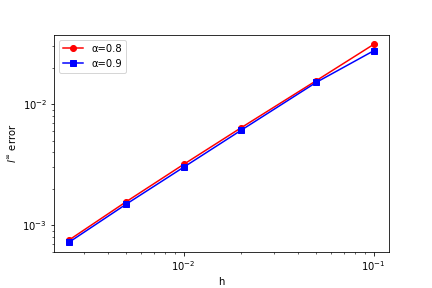 Figure 1
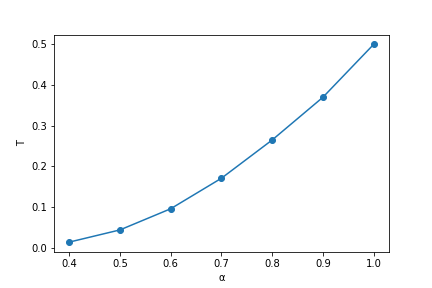 Figure 2
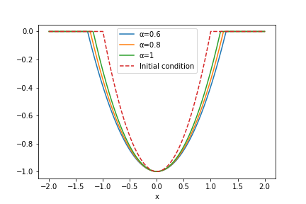 Figure 3
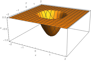 Figure 4
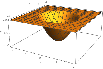 Figure 5
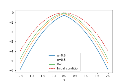 Figure 6
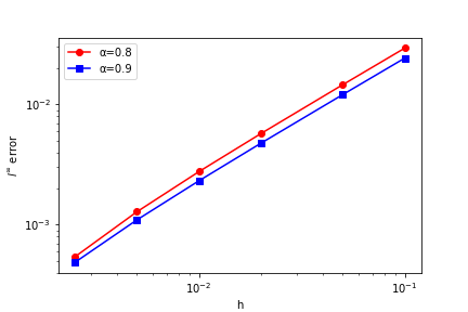 Figure 7
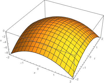 Figure 8
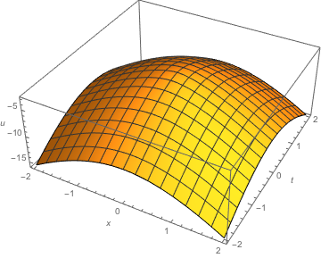 Figure 9
Peer Reviews
No public reviews on file for this paper yet. If you reviewed it on a platform where reviews are public (OpenReview, ICLR, NeurIPS, ICML), you can paste yours below so the community can read it here.
Videos
No videos yet. Explain this paper in a talk, walkthrough, or lecture? Add one.
Taxonomy
TopicsFractional Differential Equations Solutions · Iterative Methods for Nonlinear Equations · Numerical methods for differential equations
††footnotetext: S. Duisembay was partially supported by KAUST baseline funds and KAUST OSR-CRG2017-3452.
Approximation of Hamilton-Jacobi equations with Caputo time-fractional derivative
Fabio Camilli111Dip. di Scienze di Base e Applicate per l’Ingegneria, “Sapienza” Università di Roma, via Scarpa 16, 00161 Roma, Italy, (e-mail: [email protected])
Serikbolsyn Duisembay222 King Abdullah University of Science and Technology (KAUST), CEMSE division, Thuwal 23955-6900, Saudi Arabia, (e-mail: [email protected])
(March 17, 2024)
Abstract
In this paper, we investigate the numerical approximation of Hamilton-Jacobi equations with the Caputo time-fractional derivative. We introduce an explicit in time discretization of the Caputo derivative and a finite difference scheme for the approximation of the Hamiltonian. We show that the approximation scheme so obtained is stable under an appropriate condition on the discretization parameters and converges to the unique viscosity solution of the Hamilton-Jacobi equation.
AMS subject classification:
35R11, 65L12, 49L25.
Keywords:
Fractional Hamilton-Jacobi equation, Caputo time derivative, finite difference, convergence.
1 Introduction
We define a class of finite difference schemes for the time-fractional Hamilton-Jacobi equation
[TABLE]
where is unit torus in . The symbol , for , denotes the Caputo derivative
[TABLE]
(note that reduces to the standard time derivative for ) and the gradient with respect to . Equation (1.1) is completed with the initial condition
[TABLE]
In recent times, there has been an increasing interest in the study of differential equations with time-fractional derivatives. Indeed, this kind of differential operators allows us to introduce new phenomena in differential models such as memory and trapping effects [13, 14, 17, 20]. Also, the numerical approximation of differential equations with fractional time-derivative has been extensively analyzed [3, 11, 12].
Since in general smooth solutions to Hamilton-Jacobi equations are not expected to exist, for equation (1.1) a theory of weak solutions, in viscosity sense, has been introduced, in [9, 15, 21] (see also [19] for a different, but closely related, notion of weak solution). Most of the results and techniques which hold in the classical case, i.e. for , have been extended to the fractional case in order to prove the well-posedness of the Hamilton-Jacobi equation (1.1).
In the classical case, one of the most important properties of the viscosity solution theory is the stability with respect to the uniform convergence (see [2]). Starting with the seminal paper [6], this property has generated an enormous literature concerning the numerical approximation of Hamilton-Jacobi equations (see for example [7, 16, 18] and reference therein). Stability with respect to the uniform convergence is inherited by viscosity solutions of the Hamilton-Jacobi equation (1.1). Following [6], we define a general class of finite difference schemes for (1.1). We show that, under an appropriate Courant–Friedrichs–Lewy (CFL) condition of the type , these schemes are monotone, stable and consistent. Moreover, relying on an adaptation of the classical Barles-Souganidis convergence Theorem [4], we prove that the numerical solutions generated by these schemes converge to the unique viscosity solution of the limit problem. In order to verify the properties of the proposed schemes, we perform several numerical tests, and to analyze the order of the approximation error, we also compute exact solutions for some time-fractional Hamilton-Jacobi equations. We have only recently become aware that a similar problem was considered in [8].
The rest of the paper is organized as follows. In Section 2, we shortly review some basic properties of the theory of viscosity solution for (1.1). Section 3 is devoted to the description of a class of finite difference schemes and their properties. In Section 4, we prove a convergence result and in Section 5 we carry out some numerical tests.
2 Viscosity solutions for Hamilton-Jacobi equation with time-fractional derivative
In this section, we briefly review definitions and some results for the continuous problem (1.1) (we refer to [9, 15] for more details).
Throughout the paper, a function on will be equivalently regarded as a function defined on which is periodic. We consider the following assumptions on the Hamiltonian and on the initial datum .
- (H1)
is continuous; 2. (H2)
there exists a modulus such that
[TABLE]
for all ; 3. (H3)
is nondecreasing for all ; 4. (H4)
is a continuous function.
For a function such that and , the Caputo time fractional derivative is defined by
[TABLE]
for any . Using integration by parts and change of variables, (2.1) can be rewritten as
[TABLE]
where
[TABLE]
By natural extension, we also define for any with . The advantage of rewriting the Caputo derivative in the form (2.2) is explained in [1, 9, 21].
For a set and a function , we denote by and the upper and the lower semi-continuous envelopes of , i.e.
[TABLE]
and , where is a the open ball of centre and radius . We also denote by (resp., ) the class of the upper semi-continuous (resp., lower semi-continuous) functions in .
We give the definition of viscosity solution for (1.1) (see [15, Definiton 2.2]).
Definition 2.1**.**
- Let . Then
- (i)
A function is said a viscosity subsolution of (1.1) in if in and
[TABLE]
whenever and satisfy
[TABLE]
- (ii)
A function is said a viscosity supersolution of (1.1) in if in and
[TABLE]
whenever and satisfy
[TABLE]
- (iii)
A function is said a viscosity solution of (1.1) in if it is both a viscosity sub- and supersolution of (1.1) in .
In the previous definition, the notation denotes the space of functions such that , and are continuous in .
For other equivalent definitions of viscosity solutions for (1.1), we refer to [9].
The first result is a comparison principle for (1.1) (see [9, Theorem 3.1]).
Theorem 2.2**.**
Assume (H1)-(H3). Let and be a subsolution and a supersolution of (1.1), respectively. If for , then on .
We also recall an existence result for viscosity solutions of (1.1) (see [9, Theorem 4.2]).
Theorem 2.3**.**
Assume (H1). Let and be a subsolution and a supersolution of (1.1) such that and on . If , then there exists a solution of (1.1) that satisfies in .
By Theorems 2.2 and 2.3, it follows an existence and uniqueness result for the solution of (1.1), (1.2) (see [9, Corollary 4.3]).
Corollary 2.4**.**
Assume (H1)-(H4). Then there exists a unique viscosity solution of (1.1) which satisfies the initial condition (1.2).
Existence and uniqueness results for the problem of (1.1), (1.2) in a bounded domain with boundary conditions in viscosity sense are discussed in [15].
3 A class of finite difference schemes
In this section we describe a finite difference scheme for the approximation of (1.1). For simplicity of notations, we assume that the Hamiltonian depends only on the state and gradient variables, i.e. , and that the dimension is equal to . The extension for general and will be clear from this special case. Moreover, we will always identify a function with its -periodic extension defined in all .
Let be a uniform grid on the torus with step , (this supposes that is an integer), and denote by a generic point in (an anisotropic mesh with steps and is possible too and we have taken only for simplicity). The value denotes the numerical approximation of the function at , , (assuming that is an integer). We also denote by the grid function taking the value at .
We start by describing the numerical approximation of the Caputo time-fractional derivative introduced in [11]. The numerical derivative is obtained by approximating the time-derivative inside the fractional integral in (2.1) via finite difference and writing in compact form the expression so obtained. We approximate by
[TABLE]
since . Defined
[TABLE]
we obtain by (3.1)
[TABLE]
where
[TABLE]
for . Thus, the approximation of the Caputo time-derivative is given by
[TABLE]
Remark 3.1**.**
Denoted by the truncation error, in [11] it is proved that
[TABLE]
where is a constant depending on the second order time-derivative of . Hence the temporal accuracy of the scheme is of order .
In the following we summarize some properties of the coefficients in (3.3)
Lemma 3.2**.**
- (i)
for . 2. (ii)
. 3. (iii)
. 4. (iv)
.
Proof.
- (i)
When , it is clear that . Consider the case where . Because of the strong concavity of the function for , by Jensen’s inequality, we have
[TABLE]
Thus, it follows that . 2. (ii)
By definition,
[TABLE] 3. (iii)
By definition,
[TABLE] 4. (iv)
We have
[TABLE]
∎
For the approximation of the Hamiltonian in (1.1) we follow the approach in [6]. We introduce the finite difference operators
[TABLE]
and define
[TABLE]
In order to approximate the Hamiltonian in equation (1.1), we consider a numerical Hamiltonian , satisfying the following conditions:
- (G1)
is nonincreasing with respect to and , and nondecreasing with respect to and .
- (G2)
is consistent with the Hamiltonian , i.e.
[TABLE]
- (G3)
is locally Lipschitz continuous.
- (G4)
There exists a constant such that
[TABLE]
Hence, recalling the approximation (3.3) of the Caputo time derivative, we consider the explicit finite difference scheme
[TABLE]
for , , where is defined as in (3.2) and
[TABLE]
In (3.7), represents the set of the values of used to compute the scheme at , except that the value itself, and is the space discretization step. The scheme is completed with the initial condition
[TABLE]
Note that depends on all the past history , of the solution.
For , the scheme (3.6) reduces to the standard finite difference approximation
[TABLE]
of the Hamilton-Jacobi equation
[TABLE]
3.1 Stability properties of the scheme
We set and we denote by the space of the grid functions on and by , , the set of the grid function on , i.e.
[TABLE]
Moreover, we set for , and for .
For , we define a map by
[TABLE]
Hence, the scheme (3.6) can be rewritten in the equivalent iterative form
[TABLE]
Definition 3.3**.**
We say that the scheme (3.10) is monotone if, for any , , we have that
[TABLE]
where the previous inequalities are intended in the sense of the comparison of components.
Since the scheme (3.10) is explicit, for the monotonicity, we need some restriction on the approximation steps and , as we will discuss later on.
Proposition 3.4**.**
Assume that the scheme (3.6) is monotone. Then, for , we have
- (i)
for any , (where we identify both with the constant function on and with the element of such that is the constant function on for any ); 2. (ii)
for any ; 3. (iii)
For the constant in (G4),
[TABLE]
where ; 4. (iv)
for any
[TABLE]
where ; 5. (v)
for any
[TABLE]
Proof.
- (i)
By Lemma 3.2, we have
[TABLE] 2. (ii)
Let and . We have, in the sense of the comparison of components,
[TABLE]
for . By monotonicity and commutativity,
[TABLE]
Hence, . Similarly, we obtain another inequality . These two inequalities yield the result. 3. (iii)
Let be a translation operator in space, that is, for for and defined in a similar way for . Then replacing the numerical Hamiltonian with defined in (3.7) in the assumption (G4) and from the part (ii) above, it follows that
[TABLE]
since . We have similar estimates for the other components of . Combining all these inequalities, we obtain the desired inequality. 4. (iv)
Using Lemma 3.2, we have
[TABLE] 5. (v)
By the consistency of scheme, it follows that . Hence, by property (ii), we have
[TABLE]
∎
Proposition 3.5**.**
Assume that (3.6) is monotone and let be a sequence generated by the scheme with the initial condition (3.8). Then
[TABLE]
where .
Proof.
For , (3.11) is true since with defined as in (3.7). Arguing by induction, assume now that (3.11) is true for . Then using the property (iv) in Lemma 3.2, we get
[TABLE]
We observe that
[TABLE]
Moreover, by the inequality for and (which follows by the concavity of the function ), we get
[TABLE]
Hence
[TABLE]
and replacing the previous inequality in (3.12), we get estimate (3.11). ∎
We discuss some classical examples of approximation scheme for Hamilton-Jacobi equations adapted to the fractional case. We consider the equation
[TABLE]
with periodic boundary condition.
Upwind scheme
Simple upwind schemes for the equation (3.13) are
[TABLE]
if is non-increasing, or
[TABLE]
if is non-decreasing. The numerical Hamiltonian is given by , in the first case, and by in the second case. In both cases, is monotone, consistent and regular if is locally Lipschitz.
Now, we establish a condition under which the scheme (3.14) is monotone. By construction, the monotonicity with respect to is obvious. Also, since by Lemma 3.2 all the coefficients are positive, the map is increasing with respect to the variable , . Moreover, (3.14) is non-decreasing with respect to if . Recalling that , we get the CFL condition
[TABLE]
for . The same condition is necessary also for (3.15).
Lax-Friedrichs scheme
The Lax-Friedrichs scheme is given by
[TABLE]
where has to be chosen in order to satisfy the CFL condition. Therefore, the numerical Hamiltonian is
[TABLE]
for and . For the monotonicity of the scheme with respect to , we need the condition
[TABLE]
and, for the monotonicity with respect to ,
[TABLE]
Then, recalling (3.2) the monotonicity of the scheme is implied by the CFL condition
[TABLE]
for .
Remark 3.6**.**
The CFL conditions (3.16) and (3.18) reduce to the classical ones for . In general, they become more and more restrictive for decreasing to . This phenomenum has been also observed in [12] in the study of approximation schemes for time-fractional conservation laws.
4 A convergence result for the finite difference scheme
In this section, we study the convergence of the scheme (3.6) following the classical stability argument in [4], where it is proved that a monotone, stable and consistent approximation scheme converges to the unique solution of the continuous Hamilton-Jacobi equations.
We recall the definition of the relaxed limit for a locally bounded sequence . The upper relaxed limit is given by
[TABLE]
while the lower relaxed limit by
We consider a sequence of approximation steps such that for and we denote with the piecewise constant extension to of the solution of the approximation scheme (3.6) corresponding to the previous parameters, i.e. if (where denotes the integer part) and such that .
Theorem 4.1**.**
Assume that satisfies (G1)-(G4), is Lipschitz continuous and, for sufficiently small and , the scheme (3.6) is monotone. As , the sequence converges locally uniformly to the unique viscosity solution of (1.1), (1.2).
We need a preliminary result about the convergence of the fractional derivative for a test function.
Lemma 4.2**.**
Let be a test function and let for . Then, defined for the discrete fractional derivative
[TABLE]
we have
[TABLE]
Proof.
Convergence properties of the discrete fractional derivative to the continuous one are already studied in [10, 11]. Here we give a different proof of the convergence result for reader’s convenience. To simplify the notation, since in this argument only the time variable is involved, we omit the dependence of on . Because of the continuity of the Caputo derivative of with respect to (see [15, Prop. 2.1]), it is sufficient to prove that
[TABLE]
Moreover, for a test function , the Caputo derivative can be defined in the standard way, see (2.1). In the rest of the proof, we omit the index and we write , and in place of , . Fix such that and let be the greatest integer such that . Then we write
[TABLE]
We estimate the two sums (multiplied by ) in (4.2) separately. For , use the integration by parts to get
[TABLE]
Hence,
[TABLE]
Observe that for . For the first term of (4.3), using the inequality for , we have the following estimate:
[TABLE]
For the second term of (4.3), we have the following estimate:
[TABLE]
where is a modulus of continuity of . Thus,
[TABLE]
Clearly, both terms converge to [math] as .
Now, we estimate the second sum in (4.2). We have
[TABLE]
where is the modulus of continuity of on . Summarizing these estimates, we conclude
[TABLE]
as . ∎
Proof of Theorem 4.1.
In order to apply the Barles-Souganidis’ convergence result (see [4]), we define for
[TABLE]
Note that, by definition, . We claim that , are, respectively, a viscosity subsolution and a viscosity supersolution of (1.1) such that for . If the claim holds, then from Theorem 2.2 it follows that and therefore is the unique viscosity solution of (1.1) in . Moreover, the definition of , implies the uniform convergence of to .
To prove the claim, we first observe that (3.11) and the continuity of implies that for . Clearly, by (3.8) we have . Moreover, if for , then define and let be such that . We have
[TABLE]
where is the Lipschitz constant of and . Passing to the limit in the previous inequality for , we get which implies, for the arbitrariness of the sequence , . We prove similarly that .
The stability of the scheme (3.10), i.e. the boundedness of the sequence bounded uniformly in , is clearly implied by Prop. 3.5.
To prove the consistency of the scheme, we claim that, given a test function and a sequence converging to for , then we have
[TABLE]
where is defined as in (4.1). The previous claim follows by Lemma 4.2 and by the equality
[TABLE]
which is consequence of the assumptions (G2)-(G3) for the numerical Hamiltonian . Hence the claim (4.4) holds and we conclude that the scheme (3.10), besides monotone, it is also stable and consistent with the continuous equation (1.1).
We prove that, by the monotonicity, stability and consistency properties of the scheme, it follows that , are, respectively, a viscosity subsolution and a viscosity supersolution of (1.1). We only show that is a subsolution, since the argument for is similar. First observe that the stability of the scheme implies that the sequence is bounded and therefore is well defined. Consider a test function such that takes a strict maximum point at . By Lemma V.I.6 in [2], there exists a sequence such that has a maximum point at , moreover and for . Set and observe that
[TABLE]
Let be such that and such that . Define , for , and let be a modulus of continuity for . By (4.5), we have
[TABLE]
for , . Hence, recalling that is the piecewise constant interpolation of the solution of (3.6) and the scheme can be rewritten in the equivalent form (3.10), by (4.6), Prop. 3.4.(i) and the monotonicity of the scheme, we have
[TABLE]
Hence
[TABLE]
and, using the consistency of the scheme and , we finally get
[TABLE]
∎
Remark 4.3**.**
Error estimates for the approximation of Hamilton-Jacobi equations with standard time derivative have been discussed by several authors (see for example [5], [6]). We aim to investigate this point in the future.
5 Explicit solutions and numerical tests
In this section, we implement Lax-Friedrichs scheme to test the convergence of the method. The problems we consider are in and therefore the convergence is not guaranteed by the results of the previous sections, which are in the periodic case. Nevertheless, as the next examples show, we obtain a correct approximation of the exact viscosity solution of the problems.
5.1 Test 1
First, we consider the following Hamilton-Jacobi equation:
[TABLE]
It is easy to verify that, if , then the unique viscosity solution of (5.1) is given by
[TABLE]
We claim that a solution of (5.1) for is given by
[TABLE]
with non-negative function to be determined. Replacing into the equation (5.1) for and taking into account the initial datum, we find that the function has to satisfy the fractional differential equation
[TABLE]
We check that (5.2) gives a viscosity solution of (5.1). Note that, since is defined as the minimum of two solutions of the equation, by [9, Lemma 4.1] it is a supersolution in . Moreover, for , is differentiable and the equation is satisfied in point-wise sense (see [9, Prop. 2.10]), hence we only have to check the viscosity subsolution condition at . Let be a test function such that has a maximum point at (for the other point we proceed in a similar way). Recalling (2.2) and, since
[TABLE]
we see that has to satisfy
[TABLE]
Moreover, and, therefore, substituting in (5.1), we get
[TABLE]
Nevertheless, to compute , we need to compute the function . We look for a solution of (5.3) in the form of a power series . Replacing in the equation (5.3) and observing that , we have
[TABLE]
A straightforward computation gives
[TABLE]
where . Replacing the previous identity in the equation (5.4), we get
[TABLE]
Collecting the terms of the same order and recalling that, by the initial condition in (5.3), , we find
[TABLE]
From the previous relations, we can iteratively compute the coefficients of the power series and we replace in (5.2). Note that for , we get the power series of . As observed in [17, Section 6.2.3] where the problem (5.3) for is studied via power series expansion, finding the convergence interval of (5.5) is not easy, but the series can be used for small values of . Indeed we numerically find that, for each , there is a critical time for which the power series converges if and diverges if . The dependence of on is presented in Fig. 1. Hence we use the representation formula (5.2), with given by (5.3), for the exact solution of (5.1) only for . For , the viscosity solution of (5.1), which is defined for any , cannot be anymore represented by means of (5.2) and we do not know if there is an alternative explicit formula. Alternatively, we can calculate by means of a numerical methods for (5.3), but we do not pursue this approach here.
The numerical solution at of (5.1) where and computed by the Lax-Friedrichs scheme with , and is provided in Fig. 2. We plot numerical solutions at for different values of in Fig. 3 (A) for . We observe the convergent behavior of the solutions as . These solutions eventually converge to the solution of the classical case.
For the convergence test, we use error defined by the maximum difference between the exact and numerical solutions over all nodes. From Fig. 3 (B), we determine that the convergence for the Lax-Friedrichs scheme under the CFL condition is linear.
5.2 Test 2
We consider the Hamilton-Jacobi equation of the form
[TABLE]
For , the unique viscosity solution of (5.6) is
[TABLE]
For , we look for a solution in the form
[TABLE]
Computing the derivatives
[TABLE]
and replacing in the equation (5.6), we get
[TABLE]
and therefore
[TABLE]
We observe that the previous formula defines a viscosity solution of the problem. Indeed, for and , is differentiable and, since it is a solution in point-wise sense, it is also a viscosity solution (see [9, Prop. 2.10]). For and , is not differentiable with respect to , hence the equation has to be verified in viscosity sense. Since behaves as near , there cannot exist a test function such that has a minimum point at , hence the supersolution condition is automatically satisfied. Moreover, for any test function such that has a maximum point at , recalling (2.2), we see that has to satisfy
[TABLE]
and . Hence, also the subsolution condition at is satisfied. For , a similar computation gives that the solution of (5.6) is given by
[TABLE]
Fig. 4 depicts the initial condition and the numerical solution at for obtained using the Lax-Friedrichs scheme in 2 dimensions. The parameter is always chosen equal to . The numerical solutions corresponding to different values of are plotted in Fig. 5 (A) for . We can see the same convergent behavior of the solutions as as in the previous part. Moreover, from the convergence test in Fig. 5 (B), we observe that the convergence to the exact solution is linear.
The reference list from the paper itself. Each links out to its DOI / PubMed record.
- 1[1] Allen, M.; Caffarelli, L.; Vasseur, A. A parabolic problem with a fractional time derivative. Arch. Ration. Mech. Anal. 221 (2016), 603-630.
- 2[2] Bardi, M.; Capuzzo Dolcetta, I. Optimal control and viscosity solutions of Hamilton–Jacobi–Bellman equations. Birkhäuser Boston Inc., Boston (1997)
- 3[3] Baleanu, D.; Diethelm, K.; Scalas, E.; Trujillo, J. J. Fractional calculus. Models and numerical methods. Series on Complexity, Nonlinearity and Chaos, 5. World Scientific Publishing Co. Pte. Ltd., Hackensack, NJ, 2017.
- 4[4] Barles G.; Souganidis, P. Convergence of approximation scheme for fully nonlinear second order equations, Asymptotic Anal. 4 (1991), 271-283.
- 5[5] Capuzzo Dolcetta, I.; Ishii, H. Approximate solutions of the Bellman equation of deterministic control theory. Appl. Math. Optim. 11 (1984), no. 2, 161-181.
- 6[6] Crandall, M. G.; Lions, P. L. Two Approximations of Solutions of Hamilton-Jacobi Equations, Math. Comp., 43 (1984), 1-19.
- 7[7] Falcone, M.; Ferretti, R. Semi-Lagrangian approximation schemes for linear and Hamilton-Jacobi equations . Society for Industrial and Applied Mathematics (SIAM), Philadelphia, PA, 2014.
- 8[8] Giga, Y; Liu, Q.; Mitake, H. On a discrete scheme for time fractional fully nonlinear evolution equations, ar Xiv:1904.06105.