Exact and Consistent Interpretation of Piecewise Linear Models Hidden behind APIs: A Closed Form Solution
Zicun Cong, Lingyang Chu, Lanjun Wang, Xia Hu, Jian Pei

TL;DR
This paper introduces OpenAPI, a closed form solution for exactly and consistently interpreting predictions of hidden piecewise linear models behind APIs, overcoming limitations of heuristic probing methods.
Contribution
The paper presents a novel closed form approach for exact and consistent interpretation of piecewise linear models behind APIs, ensuring reliable explanations without access to model parameters.
Findings
OpenAPI provides exact interpretations of model predictions.
The method guarantees consistency across different inputs.
Experiments validate the accuracy and reliability of the approach.
Abstract
More and more AI services are provided through APIs on cloud where predictive models are hidden behind APIs. To build trust with users and reduce potential application risk, it is important to interpret how such predictive models hidden behind APIs make their decisions. The biggest challenge of interpreting such predictions is that no access to model parameters or training data is available. Existing works interpret the predictions of a model hidden behind an API by heuristically probing the response of the API with perturbed input instances. However, these methods do not provide any guarantee on the exactness and consistency of their interpretations. In this paper, we propose an elegant closed form solution named OpenAPI to compute exact and consistent interpretations for the family of Piecewise Linear Models (PLM), which includes many popular classification models. The major idea is…
Click any figure to enlarge with its caption.
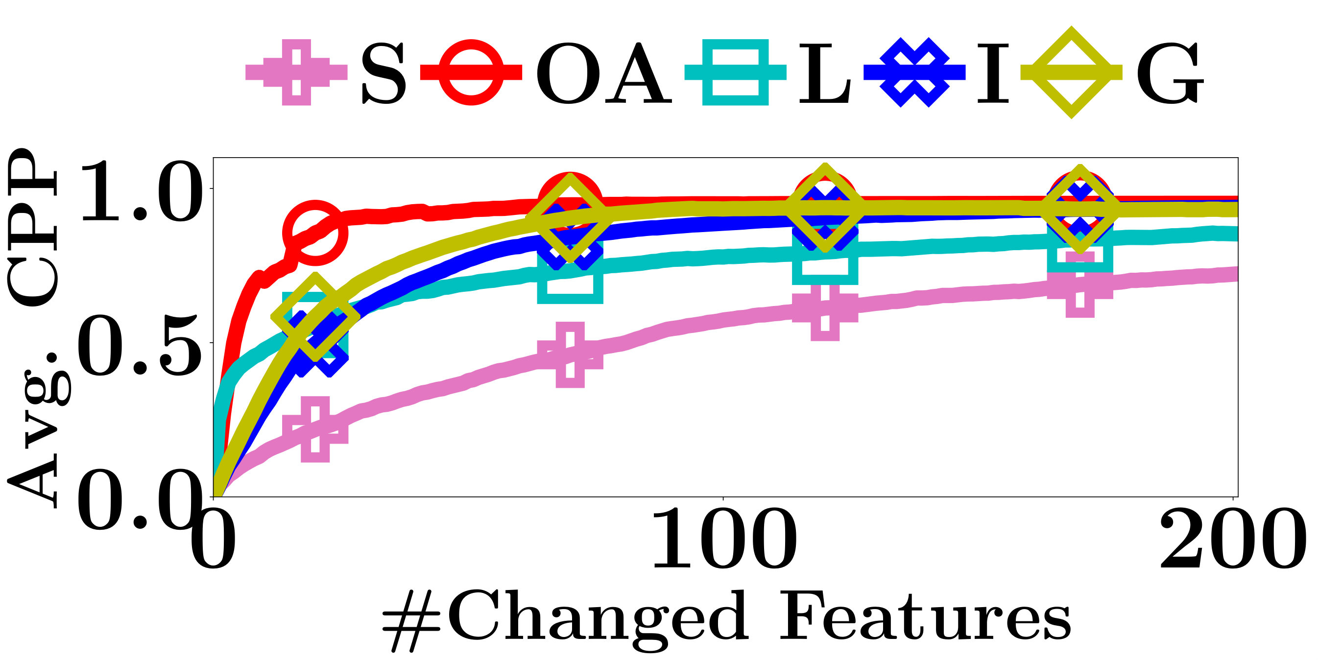 Figure 1
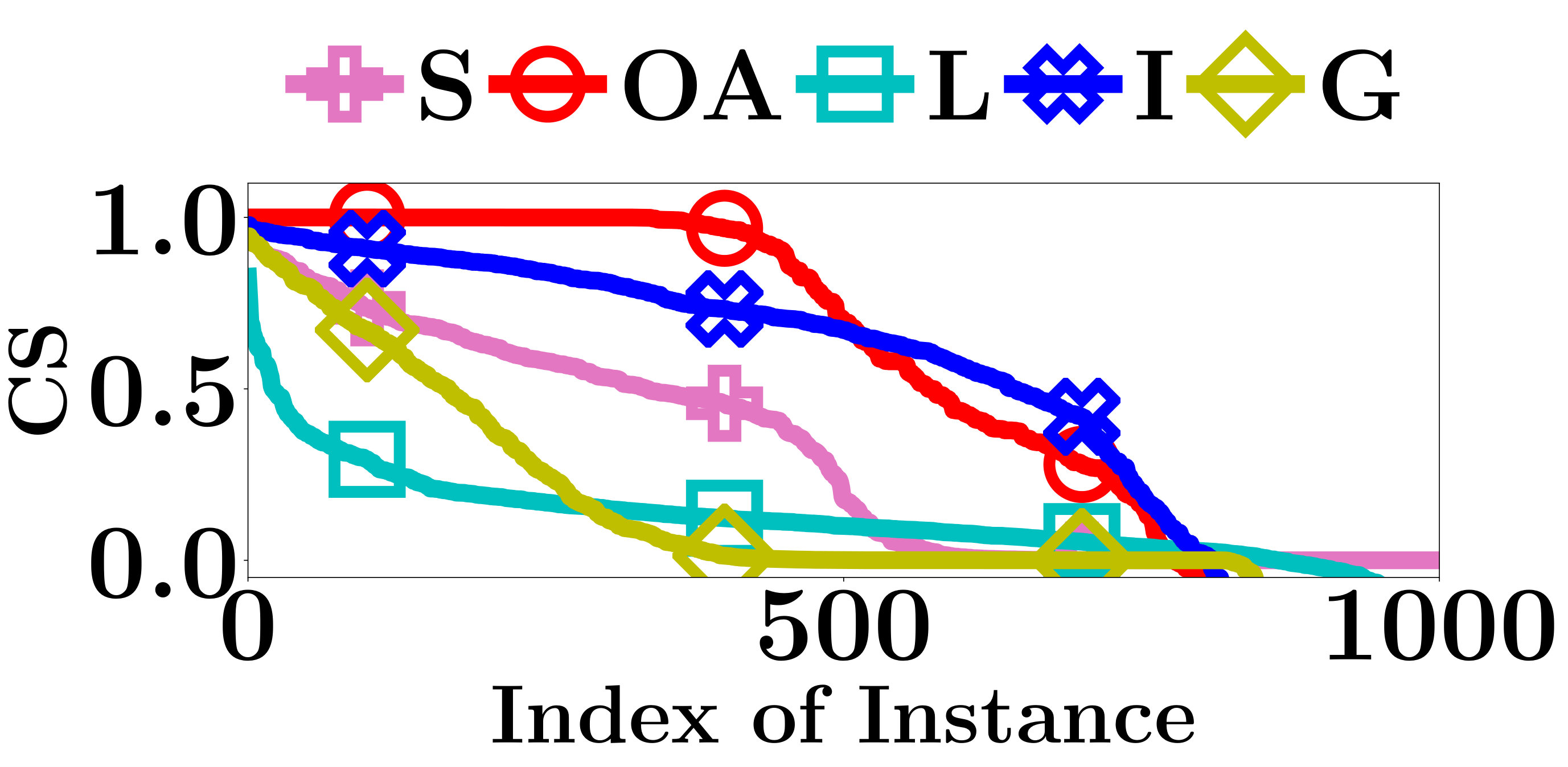 Figure 2
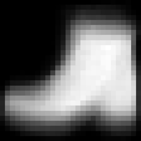 Figure 3
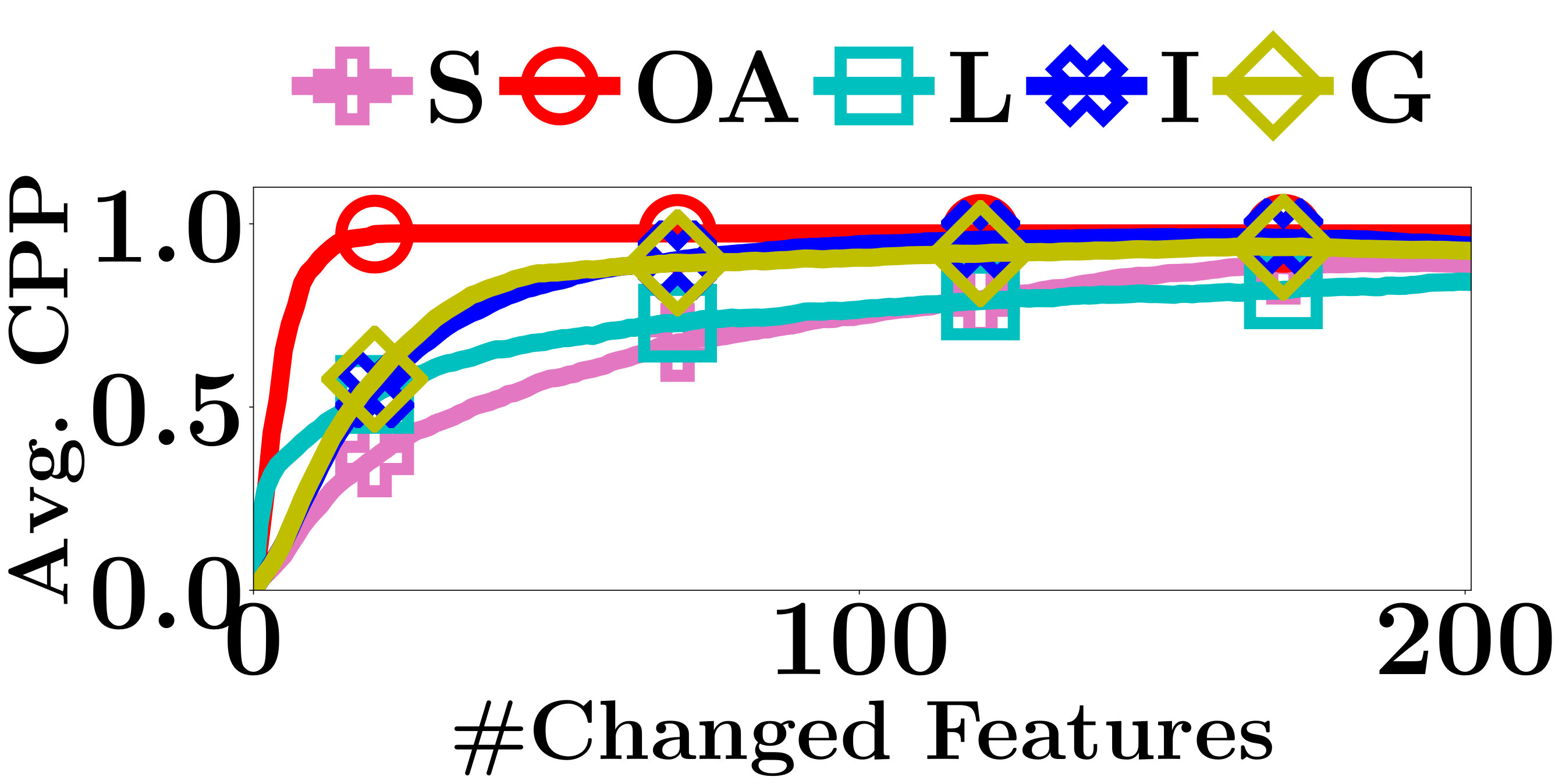 Figure 4
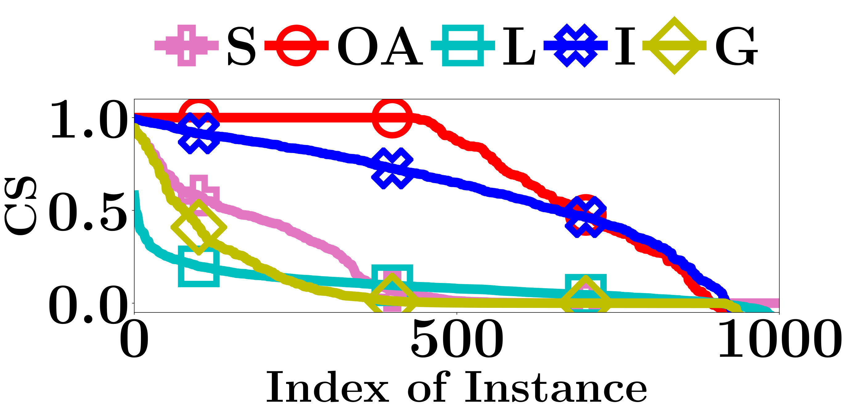 Figure 5
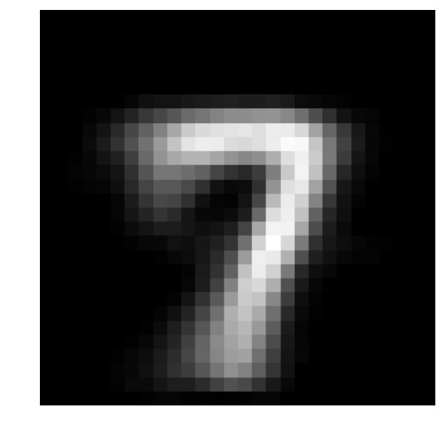 Figure 6
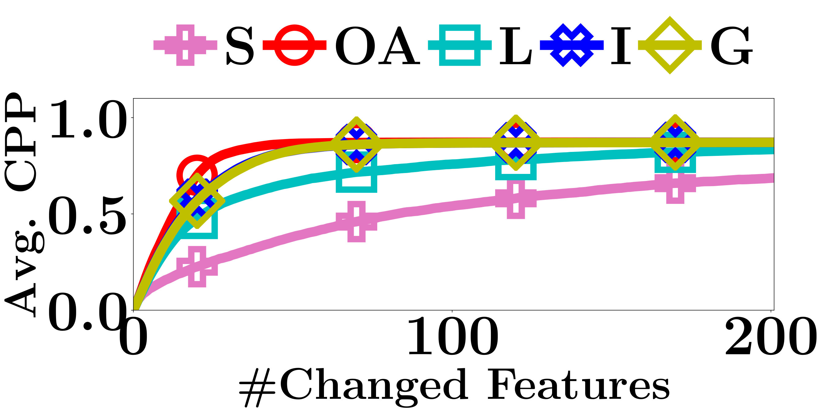 Figure 7
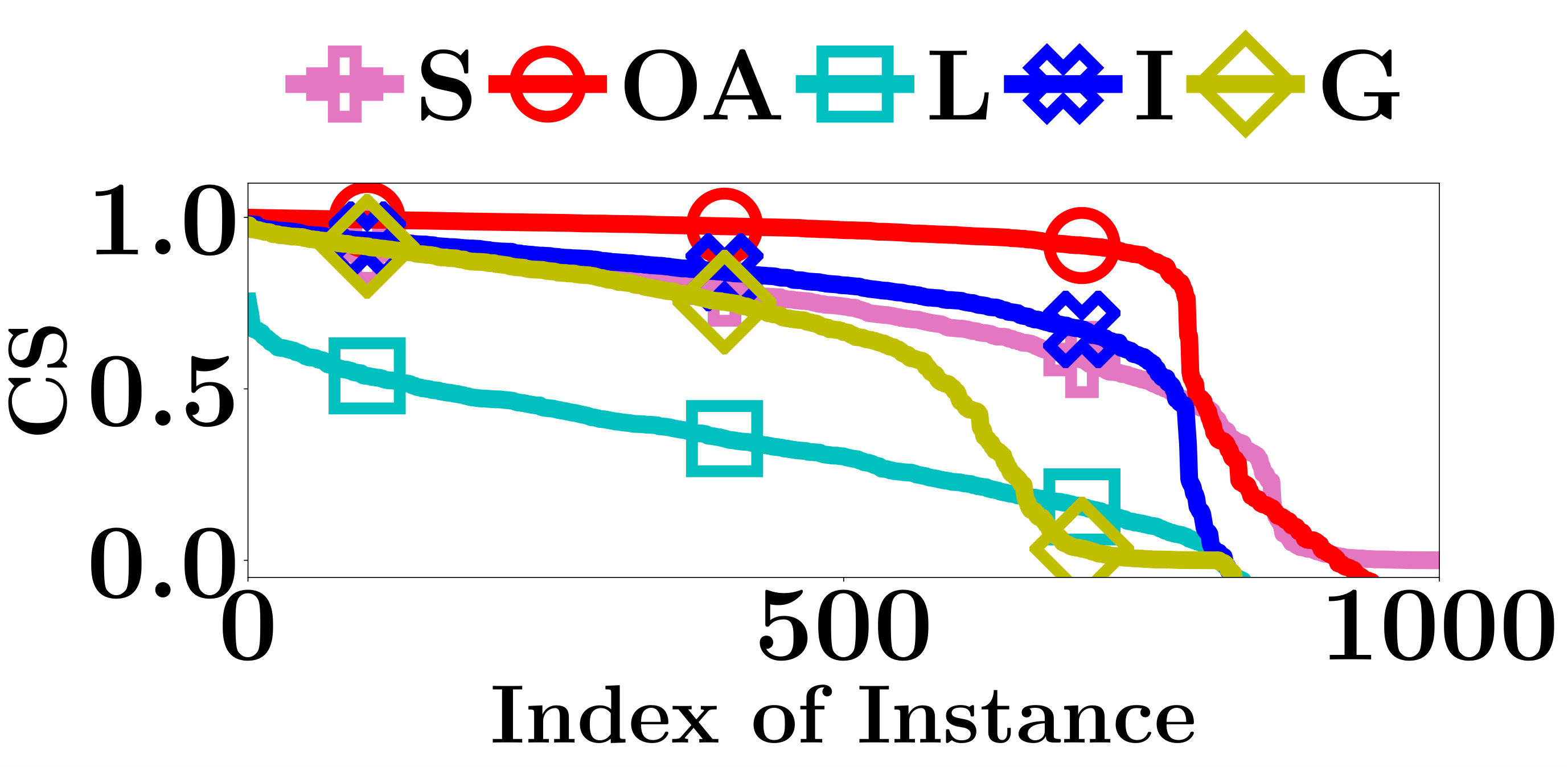 Figure 8
 Figure 9
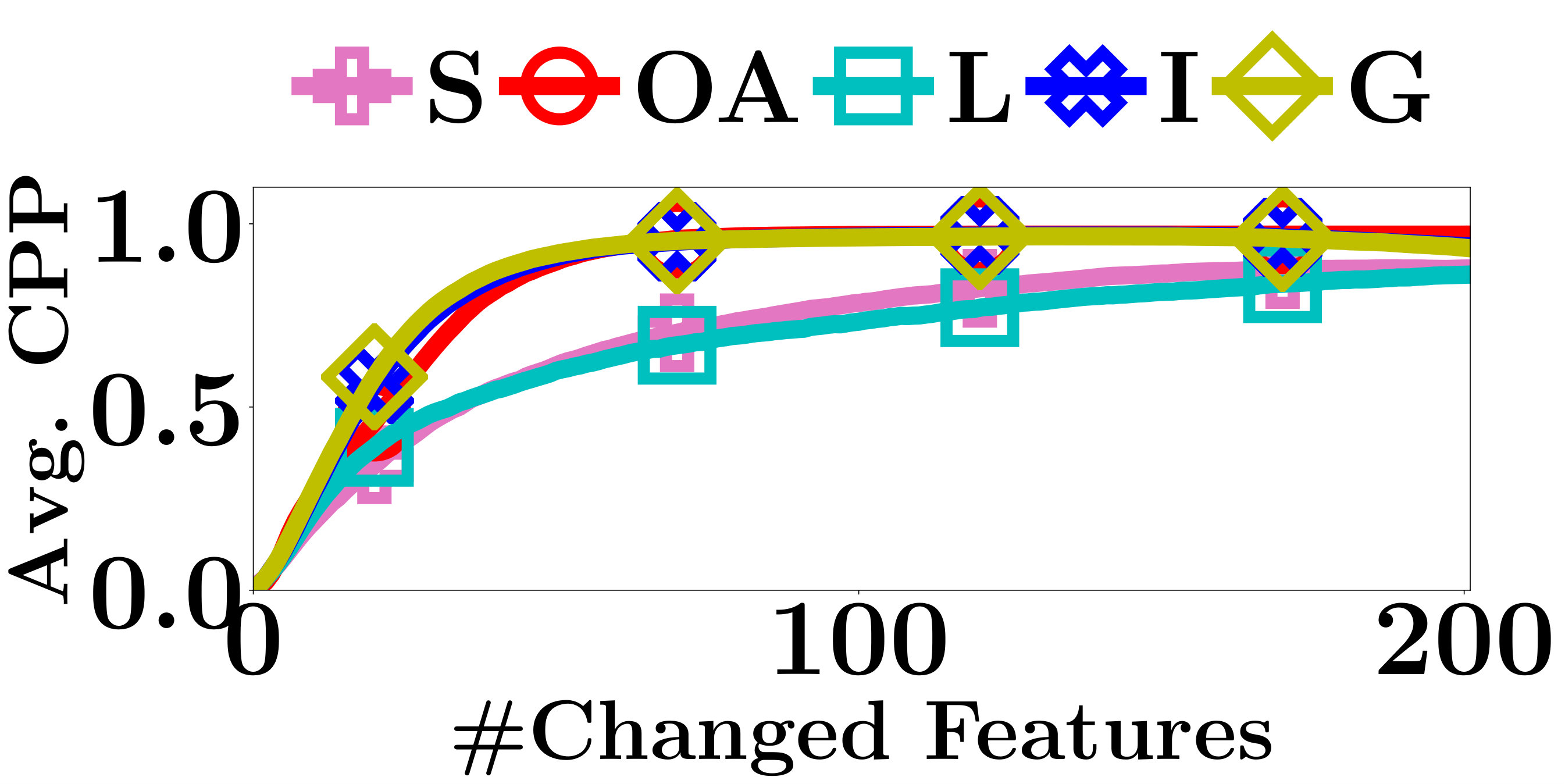 Figure 10
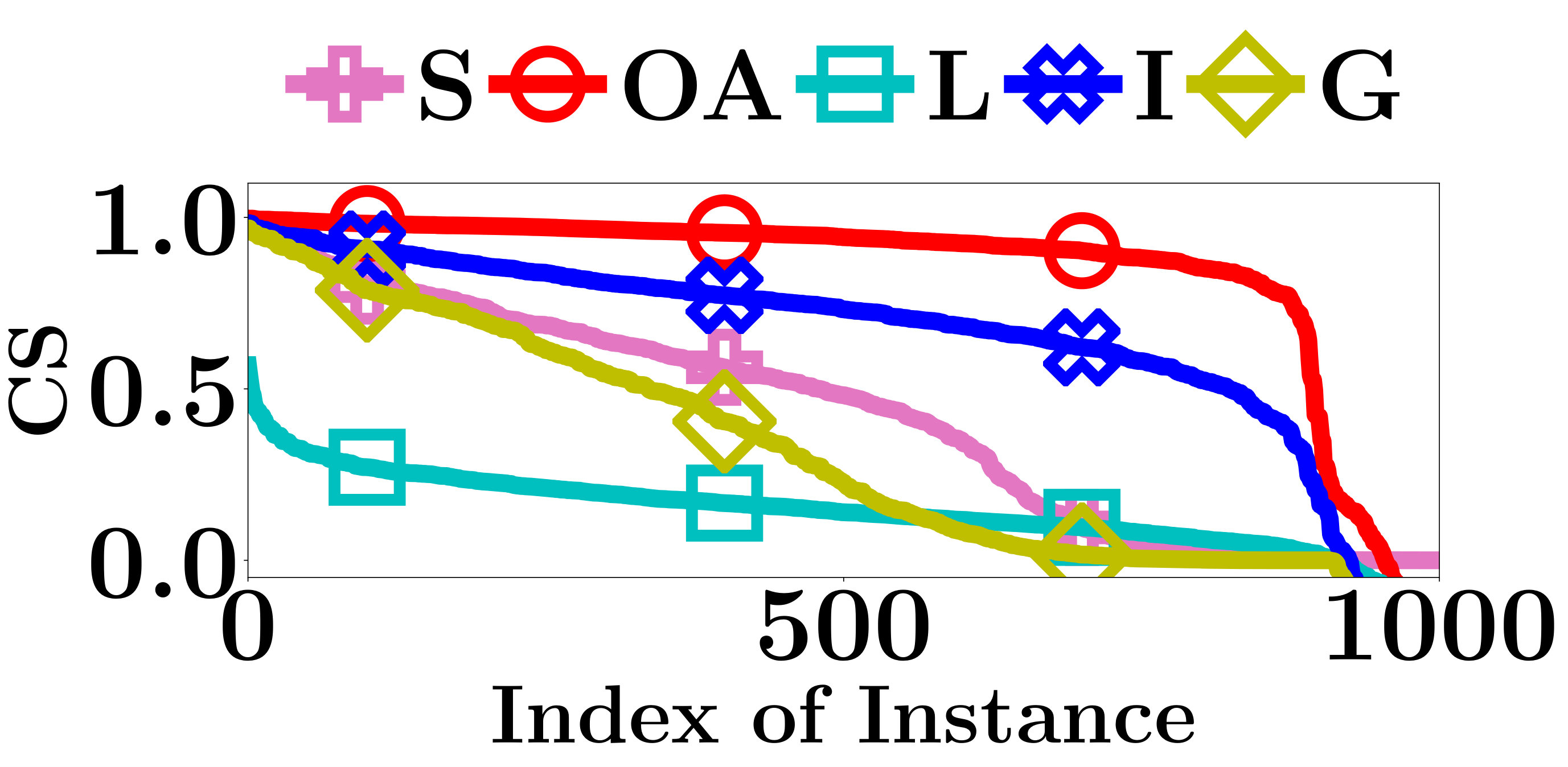 Figure 11
 Figure 12
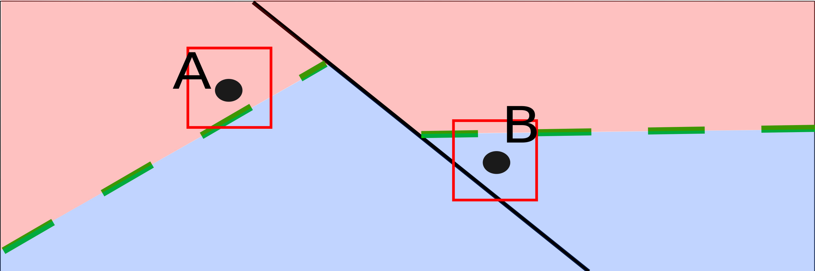 Figure 13
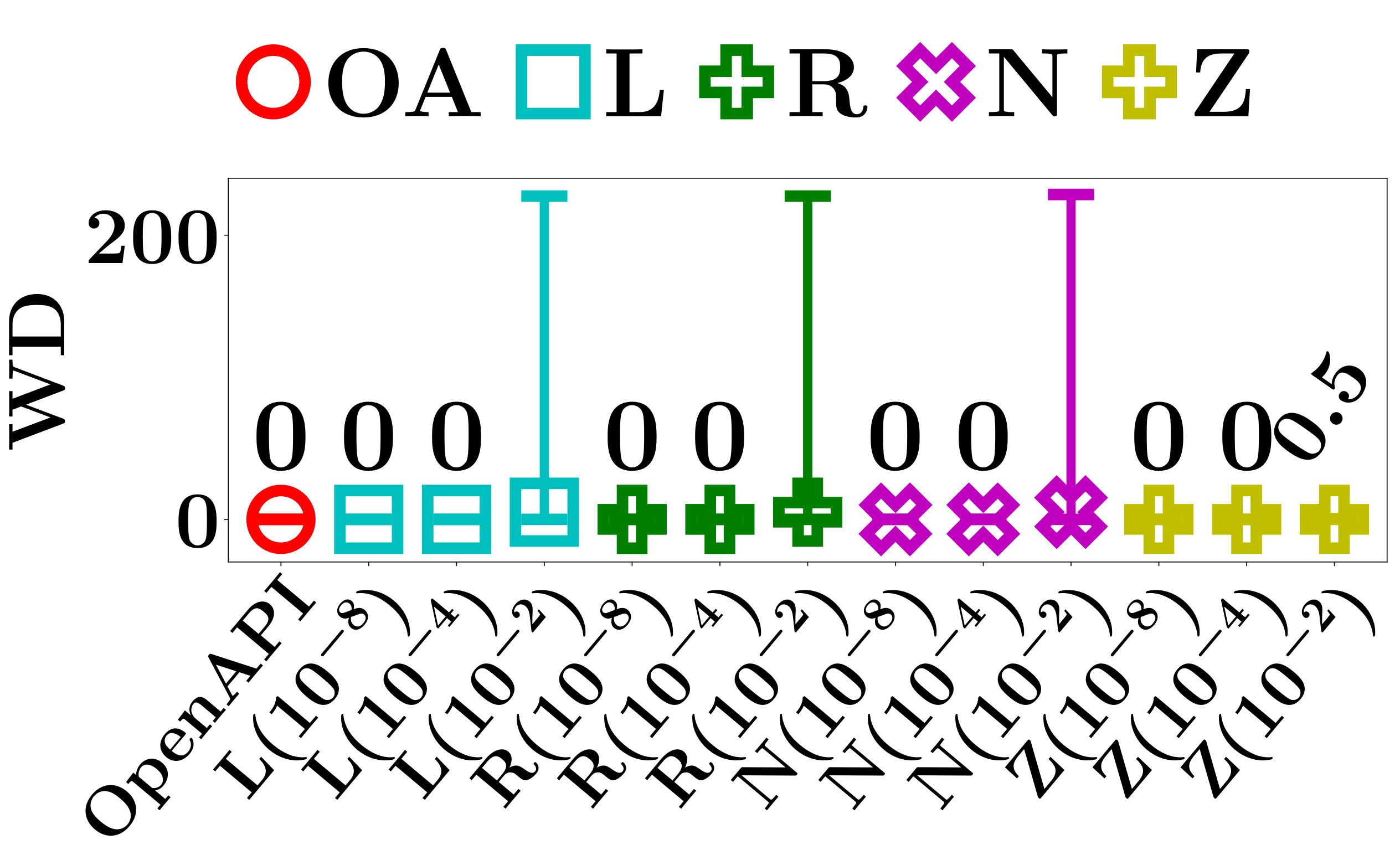 Figure 14
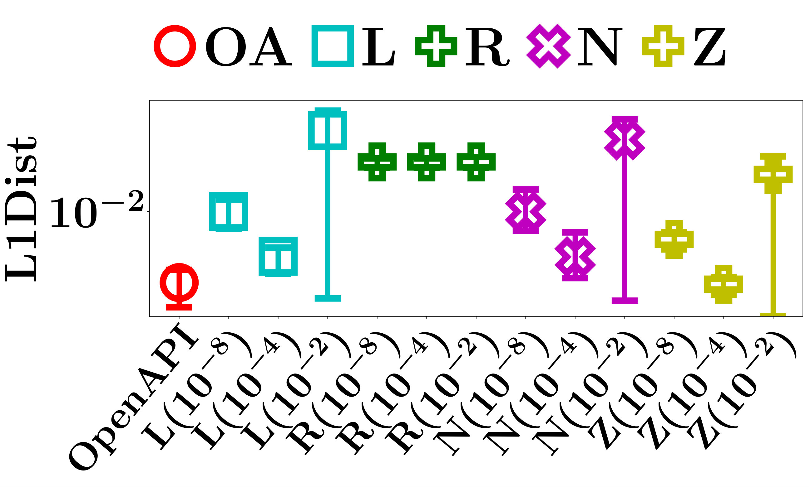 Figure 15
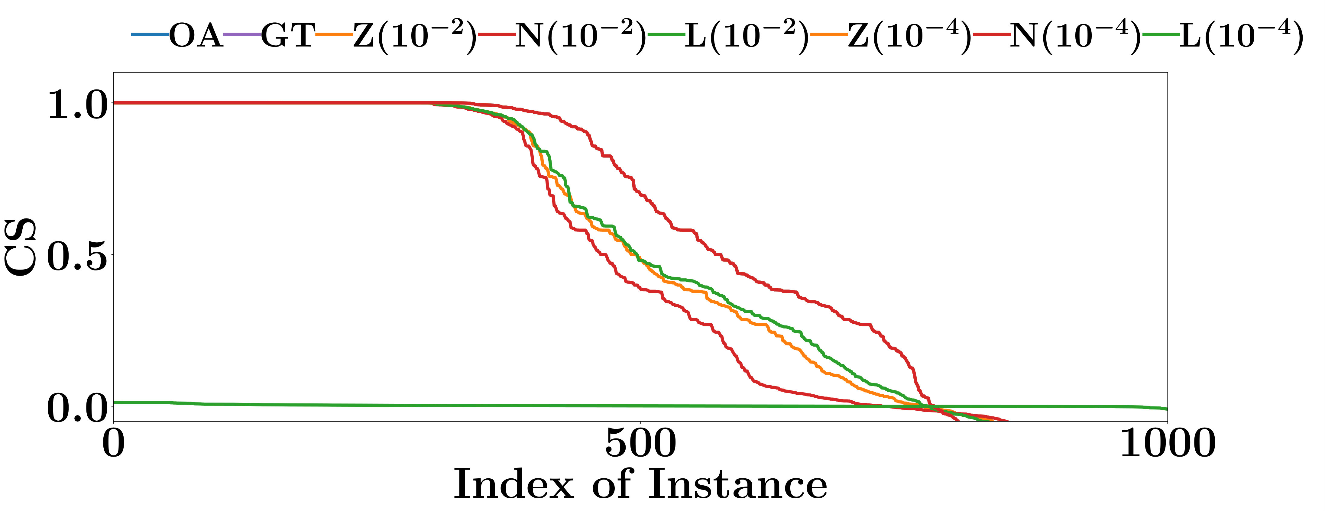 Figure 16
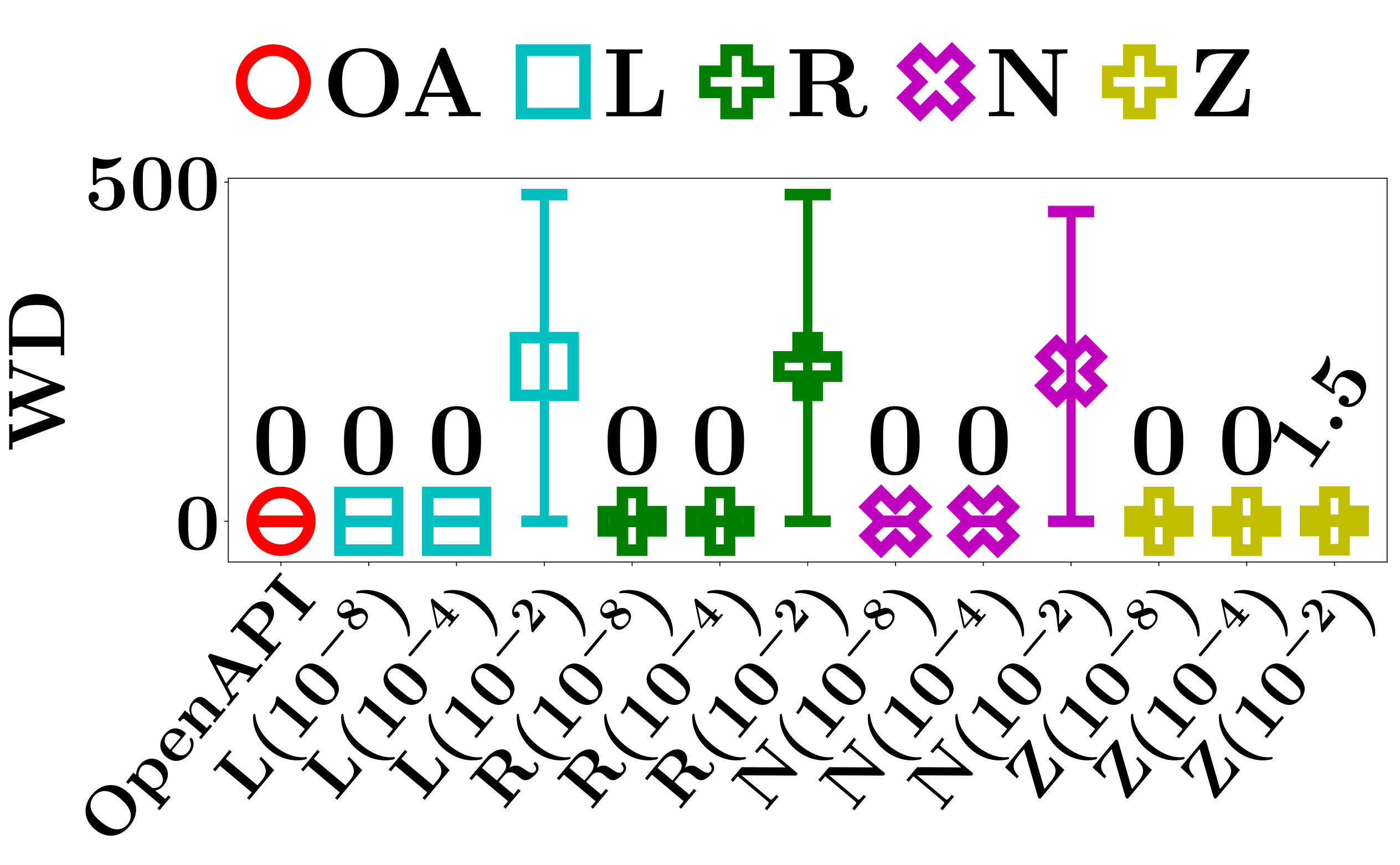 Figure 17
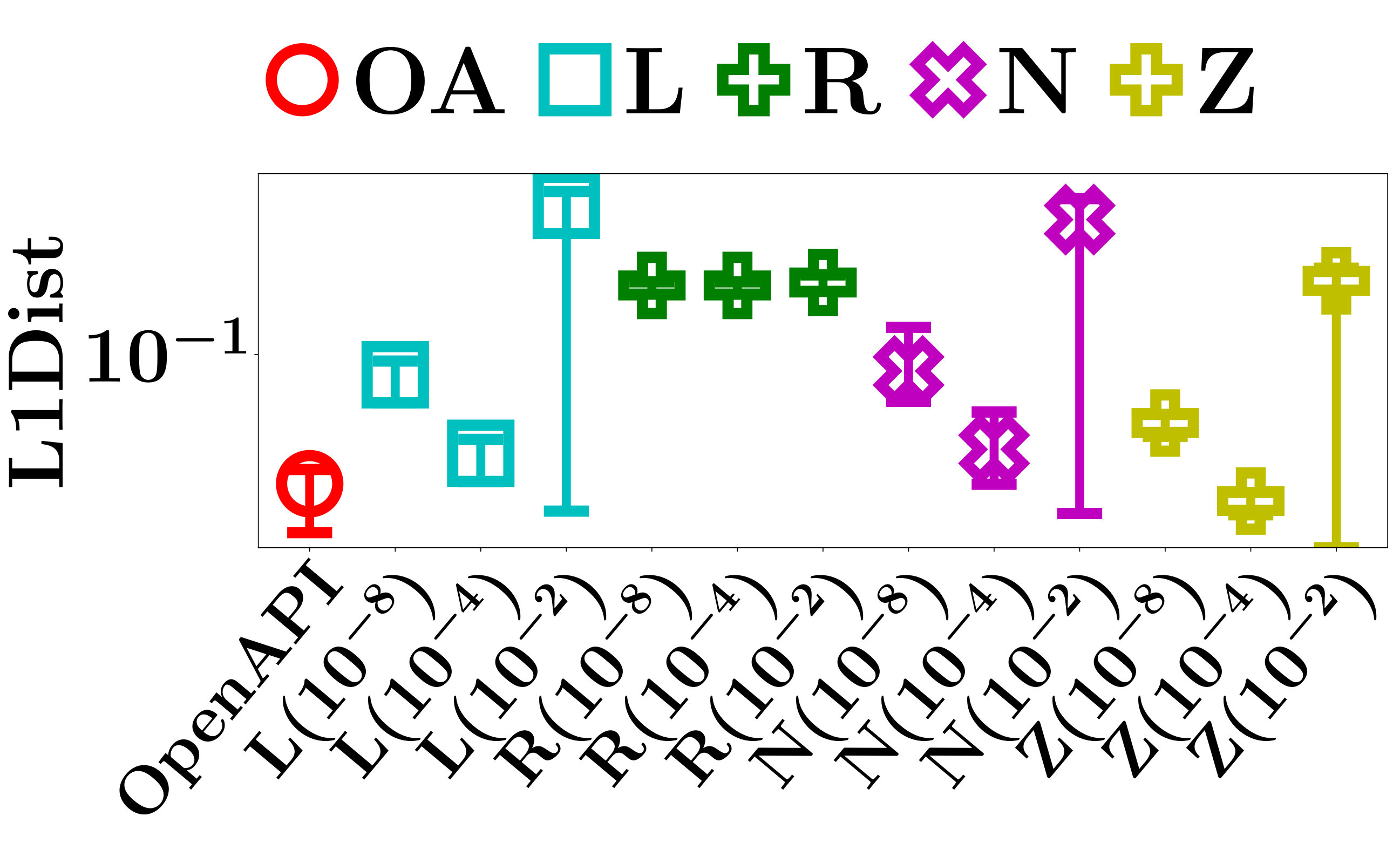 Figure 18
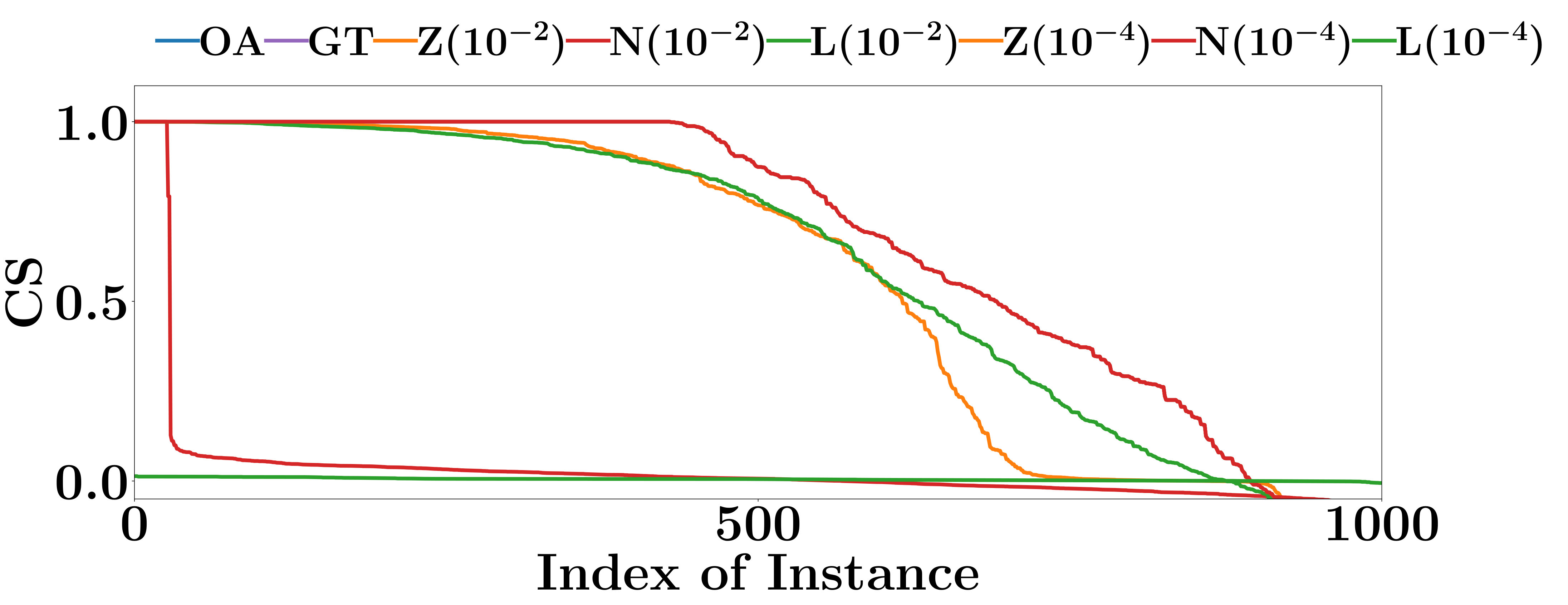 Figure 19
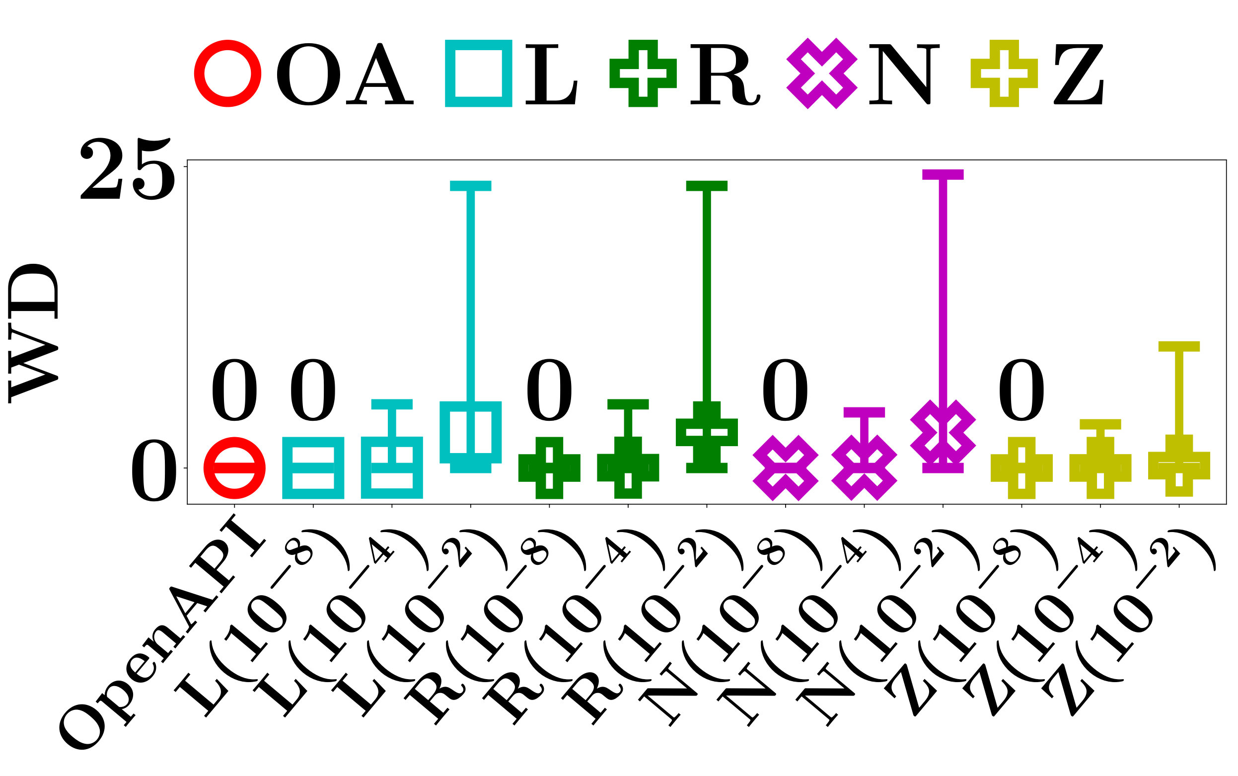 Figure 20
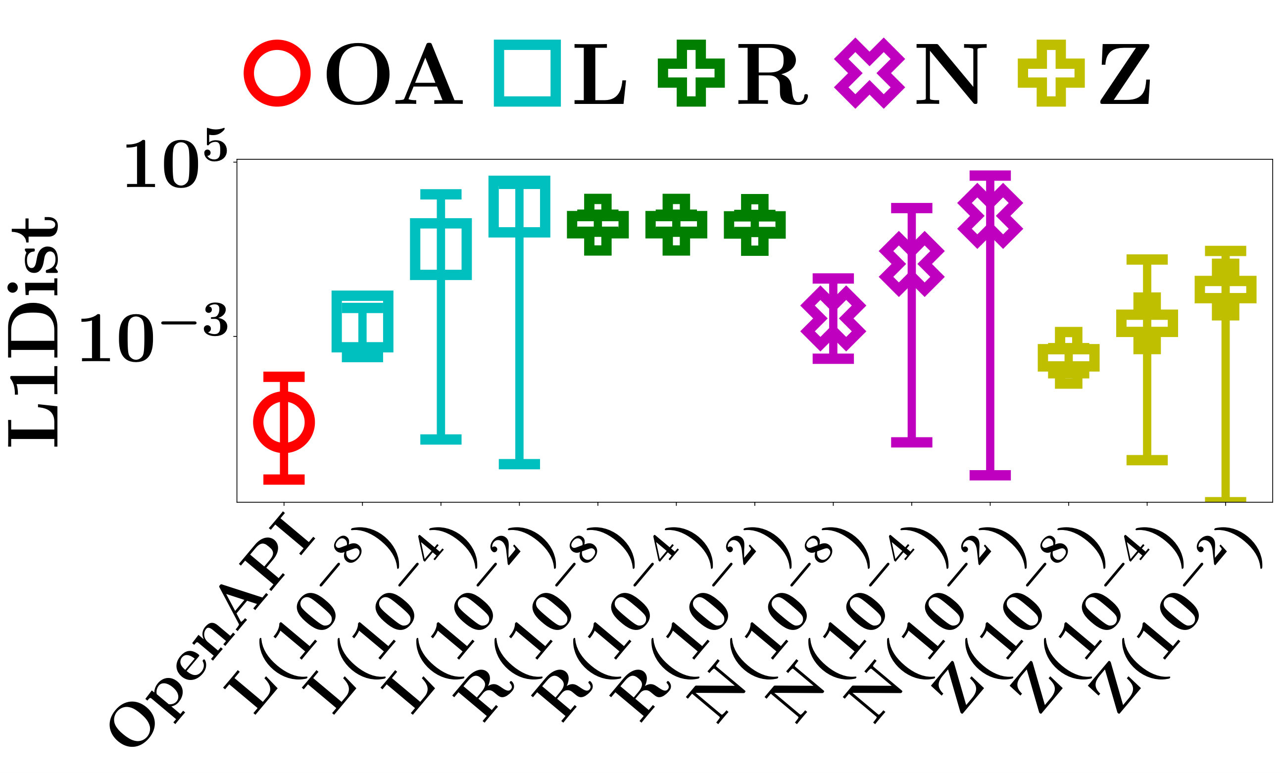 Figure 21
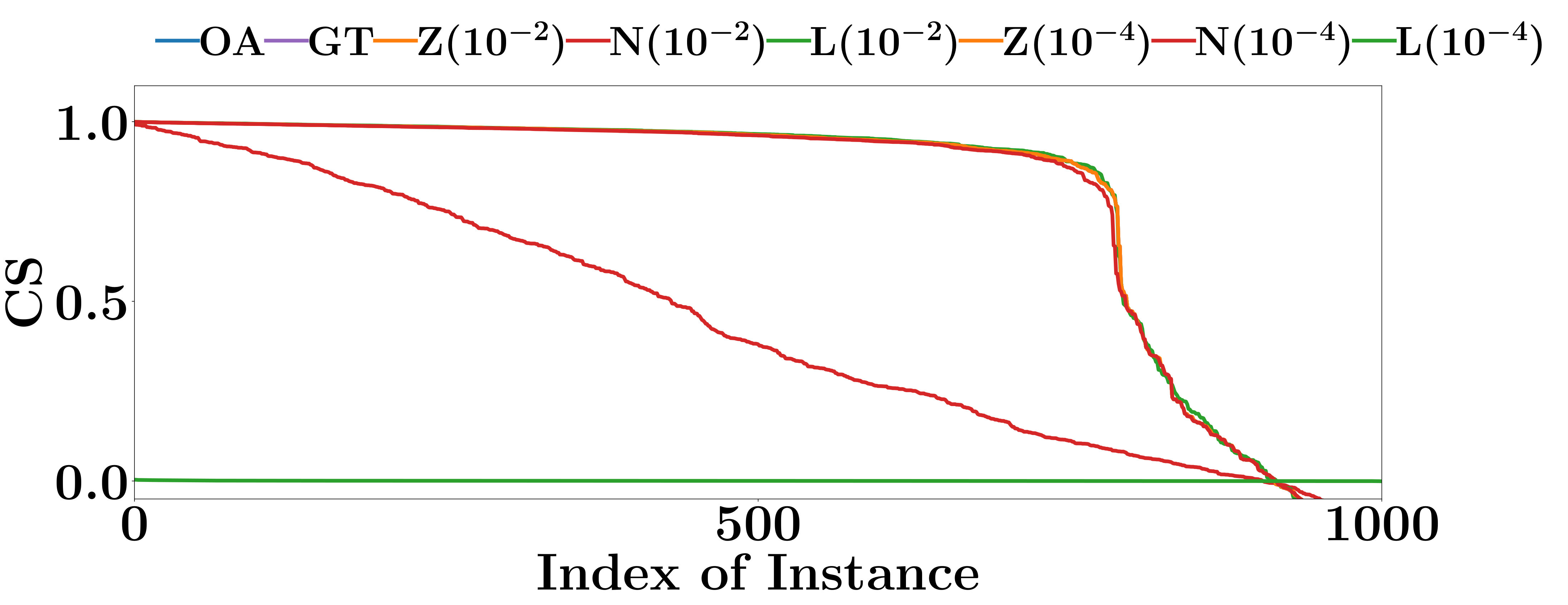 Figure 22
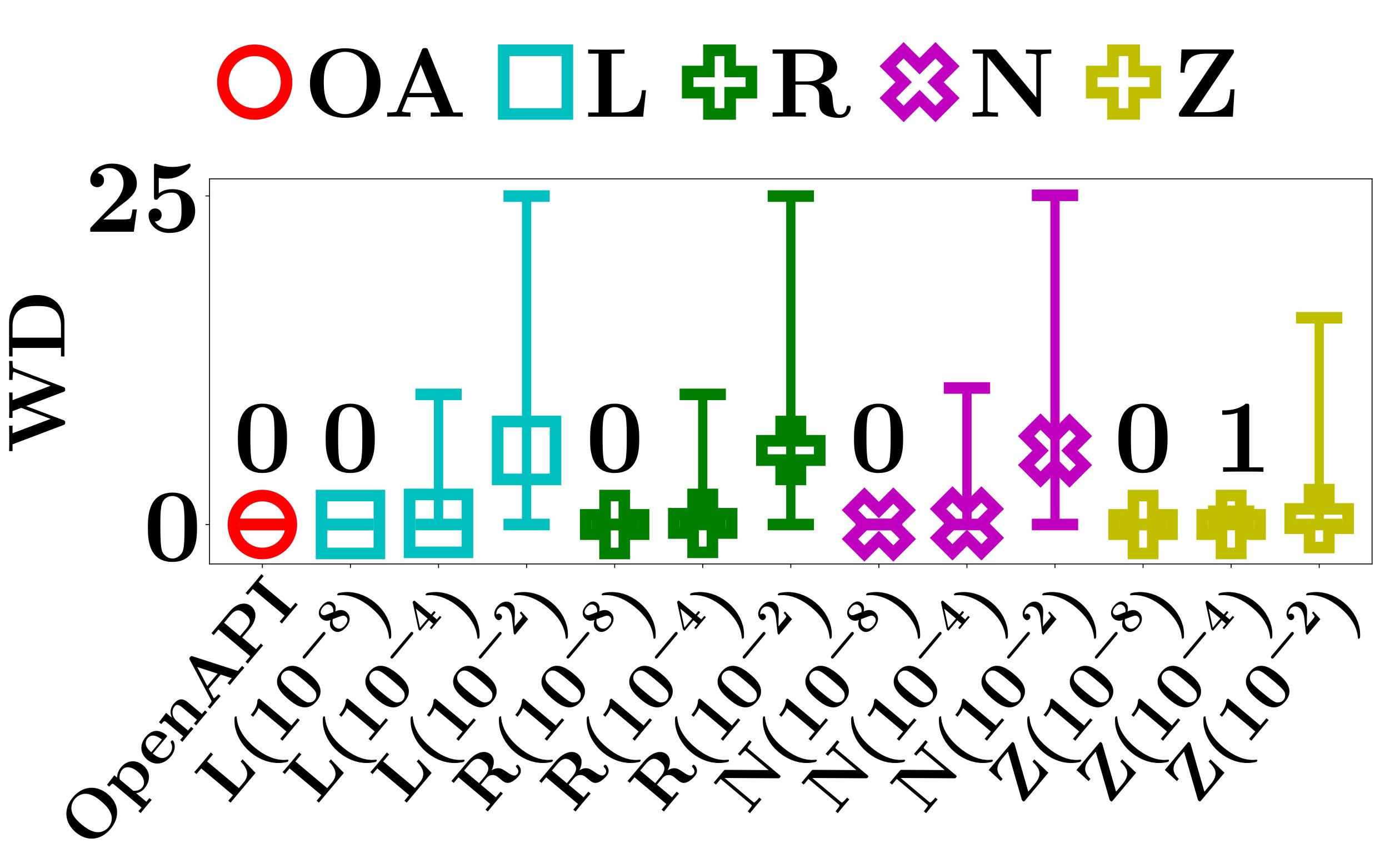 Figure 23
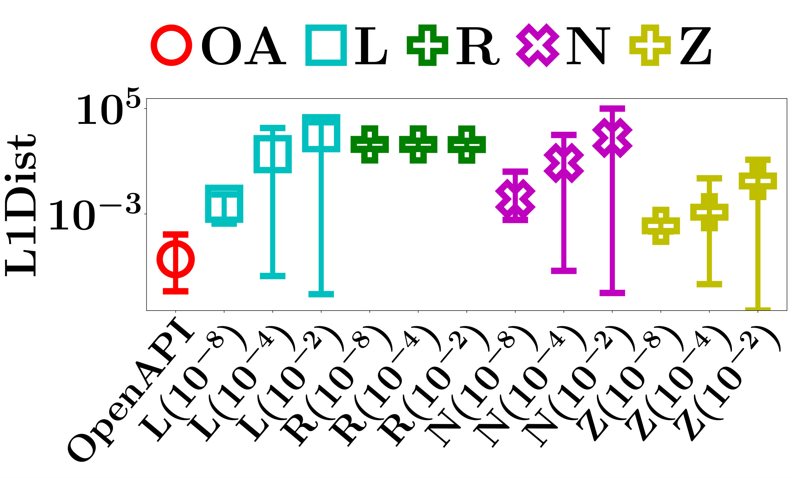 Figure 24
 Figure 25
| Data Sets | FMNIST | MNIST | ||
| Train | Test | Train | Test | |
| PLNN | 0.888 | 0.865 | 0.980 | 0.971 |
| LMT | 0.950 | 0.870 | 0.991 | 0.949 |
| Data Set | FMNIST | MNIST |
|---|---|---|
| LMT | 6.0 | 8.6 |
| PLNN | 10.3 | 10.8 |
Peer Reviews
No public reviews on file for this paper yet. If you reviewed it on a platform where reviews are public (OpenReview, ICLR, NeurIPS, ICML), you can paste yours below so the community can read it here.
Code & Models
Videos
No videos yet. Explain this paper in a talk, walkthrough, or lecture? Add one.
Taxonomy
TopicsAdversarial Robustness in Machine Learning · Explainable Artificial Intelligence (XAI) · Machine Learning and Data Classification
Exact and Consistent Interpretation of Piecewise Linear Models Hidden behind APIs: A Closed Form Solution
Zicun Cong*∗, Lingyang Chu§, Lanjun Wang§, Xia Hu∗, Jian Pei∗*
*∗*Simon Fraser University, Burnaby, Canada
§ Huawei Technologies Canada Co., Ltd., Burnaby, Canada
Emails: {zcong, huxiah, jpei}@sfu.ca, {lingyang.chu1, lanjun.wang}@huawei.com
Abstract
More and more AI services are provided through APIs on cloud where predictive models are hidden behind APIs. To build trust with users and reduce potential application risk, it is important to interpret how such predictive models hidden behind APIs make their decisions. The biggest challenge of interpreting such predictions is that no access to model parameters or training data is available. Existing works interpret the predictions of a model hidden behind an API by heuristically probing the response of the API with perturbed input instances. However, these methods do not provide any guarantee on the exactness and consistency of their interpretations. In this paper, we propose an elegant closed form solution named OpenAPI to compute exact and consistent interpretations for the family of Piecewise Linear Models (PLM), which includes many popular classification models. The major idea is to first construct a set of overdetermined linear equation systems with a small set of perturbed instances and the predictions made by the model on those instances. Then, we solve the equation systems to identify the decision features that are responsible for the prediction on an input instance. Our extensive experiments clearly demonstrate the exactness and consistency of our method.
I Introduction
More and more machine learning systems are deployed as cloud services to make important decisions routinely in many application areas, such as medicine, biology, financial business, and autonomous vehicles [14]. As more and more decisions in both number and importance are made, the demand on clearly interpreting these decision making processes is becoming ever stronger [16]. Accurately and reliably interpreting these decision making processes is the key to many essential tasks, such as detecting model failures [1], building trust with public users [34], and preventing models from unfairness [48].
Many methods have been proposed to interpret a machine learning model (see Section II for a brief review). Most of those methods are applicable only when they have full access to training data and model parameters. Unfortunately, they cannot interpret decisions made by machine learning models encapsulated by cloud services, because service providers always protect and hide their sensitive training data and predictive models as top commercial secrets [44]. More often than not, only application program interfaces (APIs) are provided to public users.
The local perturbation methods [34, 35, 7, 11] are developed to interpret predictive models that only APIs but no training data or model parameters are known. The major idea is to identify the decision features of a model by analyzing the predictions on a set of perturbed instances that are generated by perturbing (i.e., slightly modifying) the features of an instance to be interpreted. However, since the space of possible feature perturbations is exponentially large with respect to the dimensionality of the feature space, those methods can only heuristically search a tiny portion of the perturbation space in a reasonable amount of time. There is no guarantee that the decision features found are exactly the decision features of the model to be interpreted [8]. The reliability of the explanations still remains an unsolved big challenge [10]. Poor interpretations may mislead users in many scenarios [35].
Can we compute exact and consistent interpretations of decisions made by predictive models hidden behind cloud service APIs? In this paper, affirmatively we provide an elegant closed form solution for the family of piecewise linear models. Here, a piecewise linear model (PLM) is a non-linear classification model whose classification function is a piecewise linear function. In other words, a PLM consists of many locally linear regions, such that all instances in the same locally linear region are classified by the same locally linear classifier [8]. The family of PLM hosts many popular classification models, such as logistic model trees [24, 42] and the entire family of piecewise linear neural networks [8] that use MaxOut [15] or ReLU family [13, 29, 19] as activation functions. For example, the implementations of the AlexNet [23], the VGG Net [40], and the ResNet [20] all belong to the family of PLM. Due to the extensive applications [26] and tremendous practical successes [23] of piecewise linear models, exact interpretations of piecewise linear models hidden behind APIs are greatly useful in many critical application tasks.
Our major technical contribution in this paper is to develop OpenAPI, a method to exactly interpret the predictions made by a PLM model behind an API without accessing model parameters or training data. Specifically, OpenAPI identifies the decision feature, which is a vector showing the importance degree of each feature, for an instance to be interpreted by finding the closed form solutions to a set of overdetermined linear equation systems. The equation systems are simply constructed using a small set of sampled instances. We prove that the decision features identified by OpenAPI are exactly the decision features of the PLM with probability . Our interpretations are consistent within each locally linear region, because OpenAPI accurately identifies the decision features of a locally linear classifier, and those decision features are the same for all instances in the same locally linear region. We conduct extensive experiments to demonstrate the exactness and consistency of our interpretations superior to five state-of-the-art interpretation methods [34, 7, 39, 38, 43].
The rest of the paper is organized as follows. We review related works in Section II, and formulate our problem in Section III. We develop OpenAPI in Section IV, and present the experimental results in Section V. We conclude the paper in Section VI.
II Related Works
How to interpret decisions made by predictive models is an emerging and challenging problem. There are four major groups of methods, briefly reviewed here.
First, the instance attribution methods find the training instances that significantly influence the prediction on an instance to be interpreted. Wojnowicz et al. [45] used influence sketching to identify the training instances that strongly affect the fit of a regression model by efficiently estimating Cook’s distance [9]. Koh et al. [22] proposed influence functions to trace the prediction of a model and identify the training instances that are the most responsible for the prediction. Bien et al. [4] proposed a prototype selection algorithm to find a small set of representative training instances that capture the full variability of a class without confusing with the other classes. Zhou et al. [49] identified the instances that dominate the activation of the same hidden neuron of a convolutional neural network, and used the common labeled concept of those instances to interpret the semantic of the hidden neuron.
The instance attribution methods rely heavily on training data, which, unfortunately, is unavailable in most of the practical scenarios where only the APIs of the predictive models are provided.
Second, the model intimating methods train a self-explaining model to intimate the predictions of a deep neural network [3, 6, 21]. Hinton et al. [21] proposed to distill the knowledge of a large neural network by training a smaller network to imitate the predictions of the large network. To make the distilled knowledge easier to understand, Frosst et al. [12] extended the distillation method [21] by training a soft decision tree to mimic the predictions of a deep neural network. Ba et al. [3] trained a shallow mimic network to distill the knowledge of one or more deep neural networks. Wu et al. [46] used a binary decision tree to mimic and regularize the prediction function of a deep time-series model. Guo et al. [18] trained a Dirichlet Process regression mixture model to approximate the decision boundary of the intimated model near an instance to be interpreted.
The model intimating methods produce understandable interpretations. They, however, cannot be directly applied to interpret models hidden behind APIs, because they cannot access training data to conduct mimic training. Moreover, since a mimic model is not exactly the same as the intimated model, the interpretations may not exactly match the real behavior of the intimated model [8].
Third, the gradient analysis methods [39, 50, 43] find the important decision features for an instance to be interpreted by analyzing the gradient of the prediction score with respect to the instance. Simonyan et al. [39] generated a class-saliency map and a class-representative image for each class of instances by computing the gradient of the class score with respect to an input instance. Zhou et al. [50] proposed CAM to find discriminative instance regions for each class using the global average pooling in Convolutional Neural Networks (CNN). Selvaraju et al. [36] generalized CAM [50] to Grad-CAM by identifying important regions of an image, i.e., a sub-matrix, and propagating class-specific gradients into the last convolutional layer of a CNN. Smilkov et al. [41] proposed SmoothGrad to visually sharpen the gradient-based sensitivity map of an image to be interpreted. Chu et al. [8] transformed a piecewise linear neural network into a set of locally linear classifiers, and interpreted the prediction on an input instance by analyzing the gradients of all neurons with respect to the instance.
The interpretations produced by the gradient analysis methods are faithful to the real behavior of the model to be interpreted. The computation of gradients, however, requires full access to model parameters, which is usually not provided by the predictive models hidden behind APIs.
Last, the local perturbation methods interpret the behavior of a predictive model in a small neighborhood of the instance to be interpreted. The key idea is to use a simple and interpretable model to analyze the predictions on a set of perturbed instances generated by perturbing the features of the instance to be interpreted. Ribeiro et al. [34] proposed LIME to capture the decision features for an instance to be interpreted by training a linear model that fits the predictions on a sample of the perturbed instances. They also proposed Anchors [35] to find the explanatory rules that dominate the predictions on a sample of perturbed instances. Fong et al. [11] proposed to interpret the classification result of an image by finding the smallest pixel-deletion mask that causes the most significant drop of the prediction score.
The local perturbation methods, on the one hand, generate interpretations easy to understand without accessing model parameters or training data. On the other hand, the interpretations may not be even correct, since the interpretation error is proportional to , where the first component represents the parameter related error, being the perturbation distance and the number of perturbed instances, and the second component is the approximate model related error of the approximate model . Parameters not well selected may lead to a large error . The perturbation distances may be so large that the target model’s behaviors on those perturbed instances are too complicated to be learned by a simple model. The approximate model related error is due to the weaker approximation capabilities of simple models. For example, a linear model cannot exactly describe the non-linear behavior of a target model.
Although existing methods can decrease the errors in their interpretations using smaller neighborhoods, more perturbed instances, and better approximate models, the errors cannot be eliminated due to the following reason. Different instances may have different applicable perturbation distances, that is, radii where the same interpretations still apply. The proper perturbation distance for an instance can be arbitrarily small, as the instance can be arbitrarily close to the boundary of the locally linear regions.
Figure 1 elaborates the subtlety. Suppose the 2-dimensional input space is separated into two regions by a PLM (the solid boundary). Each region has a unique linear classifier whose decision boundaries are the dashed lines. The two red solid boxes of the same size represent the neighborhoods of two instances, and . As the neighborhood of completely falls into a class region of the PLM, the PLM behaves linearly there. Thus, the existing methods can obtain accurate interpretations for the prediction on by applying a simple model to analyze the perturbed instances from the neighborhood. However, the neighborhood of overlaps the decision boundary and thus the PLM does not behave linearly in the neighborhood of . Consequently, the existing methods cannot find a simple model performing exactly the same as the PLM.
The existing methods rely on a user defined perturbation distance. However, without accessing the parameters of a target model, it is impossible to find a universally applicable perturbation distance. One may wonder whether we can shrink the neighborhood size adaptively until the approximate models perfectly fit the perturbed instances. Unfortunately, the numerical optimization techniques used to train the approximate models, such as gradient descent, do not allow the current methods to reach the exact solutions [17].
The fact that existing methods cannot guarantee exactness of interpretations prevents them from being trusted by users. When the internal parameters of a target model are unavailable, users cannot verify the correctness of the interpretations. Therefore, users cannot tell whether an unexpected explanation is caused by the misbehavior of the model or by the limitations of the explanation methods [10].
In this paper, we develop OpenAPI to overcome the shortage. OpenAPI guarantees to find the exact decision features of the model to be interpreted with probability , and thus leads to a significant advantage on producing exact and consistent interpretations for the PLMs hidden behind APIs.
III Problem Definition
Denote by a piecewise linear model (PLM), and by an input instance of , where is a -dimensional input space. is also called an instance for short. The output of is , where is a -dimensional output space, and is the total number of classes.
A PLM works as a piecewise linear classification function that maps an input to an output . Denote by the -th locally linear region of such that operates as a locally linear classifier in .
Denote by the number of all locally linear regions of . Then, forms a partition of , that is, , and when . For common PLMs such as logistic model trees [24, 42] and piecewise linear neural networks [28, 8, 31], the number of locally linear regions is finite.
Without loss of generality, we write the locally linear classifier in as
[TABLE]
where is a -by- dimensional coefficient matrix of , is a -dimensional bias vector, and is a probabilistic scoring function, which can be sigmoid and softmax for binary classification and multi-class classification, respectively. Since the softmax function is the general form of the sigmoid function, we assume to be the softmax function by default, and write the complete form of as follows.
[TABLE]
Given an input instance , without loss of generality, denote by the locally linear region that contains , the classification on is uniquely determined by the locally linear classifier . For the sake of simplicity, we omit the subscript when it is clear from the context, and write the classification result of as
[TABLE]
Following a principled approach of interpreting a machine learning model [5, 34, 7], we regard an interpretation on the classification result of an input instance as the decision features that classify as one class and distinguish from the other classes. The formal definition of decision features will be discussed in Section IV-A. Formally, we define the task to interpret PLMs hidden behind APIs as follows.
Definition 1**.**
Given the API of a PLM and an input instance , for each class , our task is to identify the decision features of that classify as class and distinguish it from the other classes.
IV Interpretation Methods
In this section, we first introduce the decision features of a PLM in classifying an instance. Then, we illustrate a naive method to compute the decision features of a PLM under an ideal case. Last, as the ideal case may not always appear, we introduce the OpenAPI method that computes the exact decision features without using any training data or model parameters.
IV-A Decision Features of a PLM
Some existing methods [2] interpret model predictions by computing the partial derivatives of model outputs with respect to input features. The partial derivatives are used as importance weights of features. However, those methods do not work well for PLMs hidden behind APIs. First, to reliably compute the exact partial derivatives, the internal parameters of PLMs are needed. Second, for all instances in the same locally linear region, the weights of the corresponding features have to be consistent, as they are classified by the same locally linear classifier[8]. However, the feature weights computed by the gradient-based methods are different for different input instances.
Based on the coefficient matrices of the locally linear classifiers, we propose a new way to interpret the predictions made by PLMs. Our proposed interpretation not only describes the behaviors of PLMs exactly but is also consistent for the predictions made by the same locally linear classifiers.
Consider the output of a PLM on an instance . For any class , the -th entry of , denoted by , is the probability to predict as class . Denote by the -th column of and by the -th entry of , we can expand the locally linear classifier and write the -th entry of as .
Following the routine of interpreting conventional linear classifiers, such as Logistic Regression and linear SVM [5], is the vector of weights for all features in predicting as class . The features with positive (negative) weights in support (oppose) to predict as class .
Denote by , , the vector of weights for all features in predicting as class . The difference between and , , identifies the features that classify as class and distinguishes from class . To be specific, as , the input features of positive values in increase the confidence of the model on class over class , and vice versa. As a result, defines the decision boundary between class and class , thus is exactly the decision features of binary classification PLMs.
For general multi-class classification PLMs (i.e., ), we interpret their predictions in the way of one-vs-the-rest. We can identify the decision features that classify as class and distinguish it from the other classes by the average of the vectors for all . Since , we can write this average of vectors as
[TABLE]
Here, the decision features are a -dimensional vector that contains the importance weight of each feature in classifying as class . A feature with a larger absolute weight in is more important than one with a smaller absolute weight in classifying as class . In addition, the signs of the weights in indicate the directions of the influences of the features on the prediction. The features of positive weights in support the predictions of the model on the class over any other classes, and vice versa. In other words, is the answer to interpreting why a PLM classifies an instance as class instead of some other classes. As is computed solely from the coefficient matrices of the locally linear classifiers, for two instances and in the same locally linear region, they have the same . This property enables our method to provide consistent interpretations for predictions made on instances from the same locally linear regions.
We can easily compute when the model parameters of a PLM are given. For example, can be easily extracted from the model parameters of the conventional PLMs such as logistic model trees [24, 42]. For piecewise linear neural networks, there is also an existing method [8] that computes in polynomial time when the model parameters are given. However, none of the above methods can be used to compute when model parameters are unavailable.
IV-B A Naive Method
To use only the API of a PLM to compute without accessing any model parameters, in this subsection, we introduce a naive method by solving determined linear equation systems. In an ideal case, the solution is exactly the same as .
Given a tuple where is an input instance and is the prediction on , our goal is to compute for by computing the set such that .
For and , denote by the difference between bias vectors and . By decomposing the softmax function of the locally linear classifier , we have
[TABLE]
which can be transformed into the following linear equation
[TABLE]
Since , and are known variables, Equation 2 contains unknown variables, which are the entries of the -dimensional vector and the scalar .
Tuple fully characterizes the behavior of a locally linear classifier in classifying classes and . If two locally linear classifiers have exactly the same for every pair and , they produce exactly the same output for the same input instance . As a result, we call the core parameters of a locally linear classifier in classifying classes and . The core parameters of the locally linear classifier for an instance is also said to be the core parameters of for short.
For any pair and , a naive method to compute the core parameters of is to construct and solve a determined linear equation system, denoted by , that consists of linearly independent linear equations with the same core parameters as .
Since we already obtain one of these linear equations from , we only need to build another linear equations by independently and uniformly sampling instances in the neighborhood of . A -dimension hypercube with edge length and as the center is defined as , where is the -th entry of . In this paper, the neighborhood of refers to the hypercube centered at . We will illustrate how to compute later in Algorithm 1.
Denote by , the -th sampled instance in the neighborhood of , and by the prediction on . Obviously, can be easily obtained by feeding into the API of a PLM. Tuple is used to build the -th linear equation of in the same way as Equation 2.
In the ideal case where the core parameters of all sampled instances are the same as the core parameters of , all linear equations in are linear equations of the same core parameters as . Therefore, we can write as
[TABLE]
where is the core parameters of in classifying classes and , and , and are rewritten as , and , respectively, for notational consistency.
Next, we prove that the linear equations in are linearly independent.
Denote by the -th entry of . We write the coefficient matrix of as a -by- dimensional square matrix
[TABLE]
where the first column stores the coefficients for variable . We prove that the linear equations in are linearly independent by showing that is a full rank matrix with probability .
Lemma 1**.**
When the perturbed instances are independently and uniformly sampled from a hypercube, the coefficient matrix of is a full rank matrix with probability .
Proof.
Denote by , the -th row of , by the sub-vector containing the last entries of , that is, . Next, we prove the lemma by contradiction.
Assume the rank of matrix is not full. The last row of matrix must be a linear combination of the other rows. Denote by the weights of a linear combination, we write .
Since the first entry of every row vector is , . Recall that is a subvector of for all , we have
[TABLE]
By plugging into Equation 4, we can derive
[TABLE]
Since Equation 5 only contains the free variables , is contained in the -dimensional subspace spanned by , , .
Since , is independently and uniformly sampled from a -dimensional continuous space, and the probability that is sampled from the -dimensional subspace is [math]. Therefore, the probability that Equation 5 holds is 0, which means cannot be represented as a linear combination of the other rows. This contradicts with the assumption that is not a full rank matrix. In sum, is a full rank matrix with probability . ∎
Lemma 1 holds as long as the perturbed instances are independently and uniformly sampled from a hypercube. By Lemma 1, is a determined linear equation system that is guaranteed to have a unique solution with probability .
By solving each of the linear equation systems in , we can easily determine the core parameters of for each pair of and . Then, we can apply Equation 1 to compute .
The naive method introduced above is applicable when all sampled instances and the instance have the same core parameters. However, since we do not know the model parameters of the PLM, we cannot guarantee that those instances have the same core parameters. In other words, the ideal case may not always hold in practice. In sequel, the naive method cannot accurately compute all the time. Indeed, when the ideal case assumption does not hold, the performance of the naive method can be arbitrarily bad.
Theorem 1**.**
Denote by the solution of . When the ideal case does not hold, the probability that is the core parameters of is [math] for at least one pair of classes and .
Proof.
Denote by , the core parameters of , and by the probability of . We only need to show for at least one pair of and .
When the ideal case does not hold, there is at least one sampled instance, denoted by , that does not have the same core parameters as . Therefore, for at least one pair of classes and .
By the definition of , satisfies
[TABLE]
If , then satisfies
[TABLE]
Therefore, a necessary condition for is that satisfies
[TABLE]
As a result, cannot be larger than the probability that satisfies Equation 6.
Recall that for at least one pair of and . The value of must fall into one of the following two cases.
Case 1: if , then . In this case, no satisfies Equation 6, thus .
Case 2: if , then is the probability that is located on the hyperplane defined by Equation 6. In this case, is still 0 because is independently uniformly sampled from a -dimensional hypercube.
In summary, . The theorem follows. ∎
In summary, the naive method only works in the idea case where all perturbed instances have the same core parameters as the input instance . The extremely strong assumption limits the method to be usable in practice. First, as discussed in Section II, it is impossible for users to heuristically select a perturbation distance that works for all instances. Second, if the perturbed instances have different core parameters, according to Lemma 1 and Theorem 1, the naive method may not obtain a correct interpretation. Next, we develop OpenAPI to overcome these weaknesses.
IV-C The OpenAPI Method
Now we are ready to introduce the OpenAPI method to reliably and accurately compute . Different from the naive method, OpenAPI adaptively shrinks the perturbation distance until it computes the exact interpretations with probability .
For any two classes and , OpenAPI computes the core parameters of by solving an overdetermined linear equation system with linear equations. Denote by the overdetermined linear equation system. We build the first linear equations of in the same way as the naive method. The -th linear equation of is built by sampling an extra instance in the neighborhood of the input instance .
Denote by , , the core parameters of in classifying classes and . We now show that, when has at least one solution, the solution is unique and is equal to every with probability .
Theorem 2**.**
For any two classes and , if has at least one solution, then the solution is unique and is exactly for any with probability .
Proof.
Denote by the linear equation system that is constructed by removing the linear equation with respect to from and keeping the rest linear equations. Obviously, any solution of is a solution of .
According to Lemma 1, the coefficient matrix of is a full rank square matrix with probability . This means that the probability that has a unique solution is .
Since has at least one solution and any solution of is a solution of , the solution of is unique, and is equal to the solution of . Next, we prove that, with probability , the solution of is exactly for any .
Denote by the unique solution of , and by the probability of . We only need to show for any .
By the definition of , satisfies
[TABLE]
Since is the unique solution of , also satisfies
[TABLE]
Therefore, must satisfy
[TABLE]
Consequently, a necessary condition for is that is located on the hyperplane defined by Equation 7. Therefore, cannot be larger than the probability that is located on . The value of must fall into one of the following three cases.
Case 1: if and , then , which means .
Case 2: if and , then no satisfies Equation 7, which means . Thus, .
Case 3: if , because is drawn from an underlying continuous distribution in the -dimensional space [30], and each , is uniformly sampled from a -dimensional hypercube, we have . Therefore, .
In summary, and the theorem follows. ∎
According to Theorem 2, if has a solution, then it is the core parameters of with probability . In this case, we can directly compute as the closed form solution to . If has no solution, we can reconstruct it by randomly sampling a new set of instances in the neighborhood of , and solve the corresponding linear equation system. This iteration of reconstructions continues until we sample a set of instances that have the same core parameters as . Then, we can find the solution to , which is with probability .
Recall that all instances within the same locally linear region have the same core parameters. If we sample instances from a proper hypercube that is contained in the locally linear region of , then the instances sampled certainly have the same core parameters as , and we are sure to find the valid solution .
Intuitively, a hypercube with smaller edge length is more likely to be contained by the locally linear region of . However, it is impractical to empirically set one value of to fit all PLMs and arbitrary instances to be interpreted, because the sizes of locally linear regions vary significantly for different PLMs, and the maximum of a proper hypercube can be arbitrarily small for an input instance that is very close to the boundary of a locally linear region. Therefore, as described in Algorithm 1, OpenAPI adaptively finds a proper hypercube by reducing the edge length by half in each iteration of reconstruction.
As long as is contained in a locally linear region, OpenAPI eventually can find a proper hypercube and compute a valid output, denoted by . If is located on the boundary of a locally linear region, then there is no proper hypercube with for , and OpenAPI may fail to return a valid output. However, since the probability that is located on the boundary of a locally linear region is 0, the probability that OpenAPI returns the valid is still . To guarantee OpenAPI terminates even in the unlikely case that is located on the boundary of a locally linear region, OpenAPI stops after a certain number of iterations, which is a system parameter. In our experiments, we set the maximum number of iterations for OpenAPI as 100. However, since the probability that is located on the boundary of a locally linear region is 0, the non-terminating case never happened in our experiments, and OpenAPI always terminates in less than 20 iterations. If OpenAPI cannot find a proper hypercube within the maximum number of iterations, the smallest edge length , which is constructed at the last iteration, will be returned.
Since OpenAPI adaptively finds a proper hypercube, the initial value of has little influence on the accuracy of OpenAPI. Thus, we simply initialize it as in our experiments.
OpenAPI has three major advantages. First, OpenAPI computes interpretations in closed form, and provides a solid theoretical guarantee on the exactness of interpretations. Second, our interpretation is consistent for all instances in the same locally linear region. This is because all instances contained in the same locally linear region have the same decision features, which are accurately identified by OpenAPI. Last, OpenAPI is highly efficient, of time complexity , where and are constants for a PLM, and is the number of iterations of reconstruction.
V Experiments
In this section, we evaluate the performance of OpenAPI by investigating the following four questions: (1) Can OpenAPI effectively explain model predictions? (2) Are the interpretations consistent? (3) How well are the perturbed instances being used for interpretations? (4) Are the computed interpretations exact?
To demonstrate that OpenAPI can effectively interpret the predictions of PLMs, we compare OpenAPI with four baseline interpretation methods, Saliency Maps [39], Gradient * Input [38], Integrated Gradient [43], and LIME [34]. The first three gradient-based methods [2] require to access the model parameters. LIME can interpret the predictions of PLMs with only API access.
Saliency Maps interprets a prediction by taking the absolute value of the partial derivative of the prediction with respect to the input features. Gradient * Input uses the feature-wise product between the partial derivative and the input itself as the interpretation for a prediction. Rather than computing the partial derivative of the input instance , Integrated Gradient computes the average partial derivatives when the input varies along a linear path from a baseline point to . LIME interprets the predictions of a classifier by training an interpretable model on the outputs of the classifier in a heuristically selected neighborhood of the input instance. We adopt the same experiment settings used in [37] and [8] for Integrated Gradient and LIME, respectively.
To evaluate the capability of interpretation with only API access to PLMs, in addition to the naive method discussed in Section IV-B, we design two more baselines by slightly extending ZOO [7] and LIME [34] as follows.
ZOO is a zeroth-order approximation method approximating the gradients of functions. It first samples pairs of instances by perturbing back-and-forth along each axis of for a heuristically fixed perturbation distance . Then, it estimates the gradient of a model with respect to by computing the symmetric difference quotient [25] between each pair of sampled instances. Equation 2 clearly shows that the derivative of with respect to is exactly . Thus, it is natural to use ZOO to estimate . Then is computed from the estimated in the same way as Equation 1.
LIME interprets predictions in the one-vs-the-rest way [34]. It is easy to extend LIME such that it uses as its interpretations. Rather than training a linear model to approximate the predicted probability of a perturbed instance, the extended LIME tries to fit of the perturbed instances. Because of the linear relationship between an instance and the corresponding value , the coefficients of the linear model are an approximation to . Similarly to ZOO, is computed from the estimated . In our experiments, two types of linear regression models are used as approximators. The one using regular linear regression is called Linear Regression LIME and the one using ridge regression is called Ridge Regression LIME.
We use the published Python codes of Integrated Gradient111https://github.com/ankurtaly/Integrated-Gradients, LIME222https://github.com/marcotcr/lime and ZOO333https://github.com/huanzhang12/ZOO-Attack. The remaining algorithms are implemented using the PyTorch library [32]. All experiments are conducted on a server with two Xeon(R) Silver 4114 CPUs (2.20GHz), four Tesla P40 GPUs, 400GB main memory, and a 1.6TB SSD running Cenos 7 OS. Our source code is published at GitHub https://github.com/researchcode2/OpenAPI.
We conduct all experiments across two public datasets, FMNIST [47] and MNIST [27]. FMNIST contains fashion images in 10 categories and MNIST contains images of handwritten digits from 0 to 9. Both datasets consist of a training set of 60,000 examples and a test set of 10,000 examples.
We represent each of the 28-by-28 gray scale images by cascading the 784 pixel values into a 784-dimensional feature vector. The pixel values are normalized to the range .
On each dataset, we train a Logistic Model Tree (LMT) [24] and a Piecewise Linear Neural Network (PLNN) [8] as the target PLMs to interpret. The classification performance of all models are shown in Table I.
Following the design in [24], we use the standard C4.5 algorithm [33] to select the pivot feature for each node and a sparse multinomial logistic regression classifier is trained on each leaf node of the tree. To prevent overfitting, we adopt two stopping criteria. A node is not further split if it contains less than 100 training instances or the accuracy of the regression classifier is greater than 99%. Since every leaf node of a LMT is a locally linear classifier, the leaf node itself corresponds to a locally linear region, and we can directly extract the ground truth decision features for an input instance from the multinomial logistic regression classifier of the leaf node containing .
To train a PLNN, we use the standard back-propagation to train a fully-connected network that adopts the widely used activation function ReLU [13]. The numbers of neurons from the input layer to the output layer are 784, 256, 128, 100 and 10, respectively. This network is used as a baseline model on the website https://github.com/zalandoresearch/fashion-mnist of FMNIST. We use OpenBox [8] to compute the locally linear regions and the ground truth decision features for an input instance of a PLNN.
Since LIME is too slow to process all instances in 24 hours, for each of FMNIST and MNIST, we uniformly sample 1000 instances from the testing set, and conduct all experiments for all methods on the sampled instances.
V-A Can OpenAPI effectively Interpret Model Predictions?
Good interpretations should be easily understood by human being. In this subsection, we first conduct a case study to illustrate the effectiveness of the interpretations. Then, we quantitatively evaluate the effectiveness of the interpretations given by OpenAPI and the four baseline methods. The three gradient-based methods are allowed to use the parameter information of the PLMs to compute their interpretations. LIME and OpenAPI are only allowed to use the APIs of the PLMs.
Following the tradition of interpretation visualization [2], we show the decision features as heatmaps, where red and blue colors indicate respectively features that contribute positively to the activation of the target output and features having a suppressing effect. The first row of Figure 2 shows the averaged images of five selected classes from FMNIST. For each class, its averaged decision features of the trained PLNN and LMT are shown in the second and third rows, respectively.
Comparing the heatmaps with their corresponding averaged original images, it is clear that the decision features legibly highlight the image parts with strong semantical meanings, like the heal of boots, the shoulder of pullovers, the collar of coats, the surface of sneakers, and the short sleeves of T-shirts. A closer look at the averaged images suggests that the highlighted parts describe the differences between one type of objects against the others.
Since the LMT is trained with sparse constraints, the decision features of the LMT are sparser than the ones of the PLNN. As a result, the PLNN captures more details of the objects. Since both the LMT and the PLNN are trained on the same training data, the decision features learnt by the LMT highlight similar image patterns as the decision features of the PLNN. This demonstrates the robustness of our proposed decision features in accurately interpreting general PLMs.
To quantitatively evaluate the effectiveness of interpretations, we adopt the evaluation method used by Ancona et al. [2]. The method assumes that a good interpretation model should identify features that are more relevant to the predictions. Therefore, modifications on those relevant features should result in sensible variations on the predictions. Following this idea, we modify the input features according to their weights in the computed interpretations as follows.
For each interpretation method, given an input instance with predicted label , we sort the input features in the descending order of their absolute weights. Based on the ranking, we proceed iteratively altering the input features one at a time and up to 200 features. As the features having positive (negative) weights support (opposite) to predict as , to decrease the confidence of a PLM on class , we replace the input features of positive and negative weights by 0 and 1, respectively. The changes on the predictions are evaluated by two metrics, the change of prediction probability (CPP) and the number of label-changed instance (NLCI) [8]. CPP is the absolute change of the probability of classifying as and NLCI is the number of instances whose predicted labels change after their features being altered.
As shown in Figure 3, Saliency Maps performs worst among all methods. The result is consistent with the conclusion in [2] that the instances may have features that opposite the predictions of some classes. Those features play an important role in interpreting the model predictions and can only be detected by signed interpretation methods. As shown in Figure 3 and mentioned by Ancona et al. [2], Gradient * Input captures important features better than Integrated Gradient. The latter involves the gradients of the unrelated instances into interpretations, therefore cannot precisely interpret the predictions. As expected, LIME performs poorer than most of the gradient-based methods due to the fact that LIME has no access to the model parameters. The lack of internal information prevents it from getting accurate interpretations. However, only with API access to the PLMs, OpenAPI outperforms the other methods most of the time, because our method computes the decision features that are exactly used by the PLMs in prediction. The good performance demonstrates the effectiveness of our method.
V-B Are the Interpretations Consistent?
Consistent interpretation methods provide similar interpretations for similar input instances, and produce fewer contradictions between interpretations. Consistency is important. For example, it is confusing if, for the instances in a locally linear region, the weights of their corresponding features are not the same, because those instances are classified by the same locally linear classifier of the PLM.
Using the same experiment settings as Chu et al. [8], we comprehensively analyze the consistency of the interpretations produced by Saliency Maps, Integrated Gradient, Gradient * Input, and OpenAPI by comparing the decision features of similar input instances.
Denote by an input instance classified as class , and by the testing instance that is the nearest neighbour of in Euclidean distance.
For an interpretation method, we measure the interpretation consistency by the Cosine Similarity (CS) between the computed interpretations of and . Apparently, a larger CS indicates a better interpretation consistency.
The CS of all compared methods are evaluated on the testing data sets of FMNIST and MNIST. As shown in Figure 4, the interpretations given by Integrated Gradient are more consistent than the other two gradient based methods. Integrated Gradient smooths the differences between the interpretations for similar instances using the average partial derivatives of a set of instances to compute its interpretations. At the same time, the smooth operation also decreases the accuracy of its interpretations. The CS of OpenAPI is better than all other methods on all PLMs and datasets. All instances contained in the same locally linear region have exactly the same decision features, and thus the CS of OpenAPI should always equal to 1 on those instances. As an input instance and its nearest neighbor in the test set may not always belong to the same locally linear region, the CS of OpenAPI is not equal to 1 for all instances in our experiments. The poor performances of the baseline methods can be anticipated, since their interpretations rely on the gradients of the input instances, and they tend to provide distinct interpretations for individual instances.
In summary, the interpretation consistency of OpenAPI is significantly better than the other baseline methods.
V-C How Well Are the Perturbed Instances?
The accuracy of all compared methods in computing of an input instance largely depends on the quality of the set of sampled instances. Here, the quality of a set of instances is good if they are contained in the same locally linear region as , and thus those instances have the same core parameters as and significantly improve the accuracy in computing .
To comprehensively evaluate the performance of the compared methods in sampling a set of good instances, we measure the quality of the sampled instances by the following two metrics.
The Region Difference (RD) measures the consistency of the locally linear regions of the sampled instances. For any input instance , if all sampled instances are contained in the same locally linear region as , then ; otherwise, .
The Weight Difference (WD) is defined as
[TABLE]
which measures the average L1 distance between of the input instance and of the -th instance in the set of sampled instances .
Apparently, a RD that is equal to [math] indicates a perfect consistency among the locally linear regions of all sampled instances. A small WD means a high similarity between the core parameters of and the sampled instances. If RD and WD are both small, the quality of the sampled instances is good, and of can be accurately computed.
We evaluate RD and WD of ZOO, Linear Regression LIME, Ridge Regression LIME, the naive method, and OpenAPI on the testing data sets of FMNIST and MNIST. For each data set, we use every testing instance as the input instance once, and evaluate RD and WD of the corresponding set of sampled instances. Figures 5 and 6, respectively, show the average RD and WD of all testing instances.
The performance of the baseline methods in RD and WD relies heavily on the heuristic perturbation distance . Since there is no effective method to set , we evaluate the performance of the baseline methods with respect to a wide range of . Specifically, we test , , and .
As shown in Figure 5, the average RD of the baseline methods increases when increases. The results verify our claim in Section IV-C that a smaller hypercube is more likely to be contained in the locally linear region of an input instance.
Since the RD of the baseline methods drops to 0 when is small, it is appealing to ask whether we can fix to a small value such that the baseline methods can always find a good sample of instances. Unfortunately, this is impossible. The volume of locally linear regions varies significantly for different PLMs. For example, as shown in Figure 5, when the perturbation distance , the RD of ZOO is [math] for LMT, but it is and for PLNN on FMNIST and MNIST, respectively. Thus, is good for LMT, but not good enough for PLNN. One may argue that conservatively can take an extremely small value in the hope that it works for both LMT and PLNN. However, since the number of locally linear regions of a PLNN is exponential with respect to the number of hidden units [28, 8, 31], the volume of some locally linear regions of a large PLNN can be arbitrarily close to zero. For any fixed value of , one can always construct a counter example that is still too big for PLNN. Even for the same PLM, the good perturbation distance may still vary significantly for different input instances, and can be arbitrarily small.
Recall that we can only access the API of a PLM, we have no knowledge about the size of the locally linear regions of the PLM. This makes it even harder to initialize an optimal value of perturbation distance that works universally on all PLMs and input instances. A much better method is to sample a set of good instances in an adaptive manner, just as what OpenAPI does.
As shown in Figures 5 and 6, the average RD and WD of OpenAPI are [math] on all data sets. This demonstrates the superior capability of OpenAPI in adaptively sampling a set of good instances.
V-D Are the Interpretations Exact?
In this subsection, we systematically study the exactness of interpretations by comparing the ground truth of the decision features of a PLM with the decision features identified by ZOO, Linear Regression LIME, Ridge Regression LIME, the naive method, and OpenAPI.
Denote by the ground truth of decision features of a PLM in classifying an input instance as class , and by the decision features computed by an interpretation method. We measure the exactness of an interpretation by L1Dist, the L1 distance between and . Obviously, a smaller L1Dist indicates a higher exactness of an interpretation.
We evaluate L1Dist of the four baseline methods and OpenAPI on the testing data sets. For each data set, we use every testing instance as the input instance, and evaluate L1Dist of the interpretations. The average, minimum and maximum L1Dist of all testing instances are reported in Figure 7.
The large L1Dist of Ridge Regression LIME on all datasets indicates that computed by the method is significantly different from of the PLMs. By carefully investigating the learned classifiers of Ridge Regression LIME, we find that when the perturbed distances are very small, the linear function used to approximate the predictions always converges to a constant function that always outputs the expected value of the predictions. The poor exactness of Ridge Regression LIME is mainly caused by the mis-selected approximate model. As a comparison, Linear Regression LIME, which has no constraints on its coefficient matrix, performs much better than its counterpart with ridge regression.
The L1Dist of the other baseline methods increases significantly when the perturbation distance becomes larger than a critical value. Since a smaller leads to a better quality of the sampled instances, it usually increases the accuracy of most baseline methods in computing . However, as discussed in Section V-C, the critical value of varies significantly for different models and instances, thus it is impossible to find a golden value of that always achieves the best L1Dist in computing the decision features of all models and instances.
We can also see that when becomes extremely small, L1Dist increases. The reason is that all methods suffer from the classical problem of softmax saturation. When an input instance is classified with a probability extremely close to and the perturbed distance becomes extremely small, the PLMs have almost the same predictions on the perturbed instances and the original instance. As a result, the computation of the decision features becomes unstable, which goes beyond the limited precision of Python in stably manipulating floating point numbers. Also, extremely small perturbations lead to linear equation systems with large condition numbers, which are hard to solve numerically. Due to the above reasons, extremely small perturbations hurt the exactness of all methods.
The computation of the decision features becomes unstable due to two reasons.
In contrast, since OpenAPI is able to find the exact decision features of a PLM with probability , it achieves the best L1Dist performance on all data sets. In addition, as shown in Table II, OpenAPI can find the exact interpretations with only a small number of iterations.
VI Conclusions
In this paper, we tackle the challenge of interpreting a PLM hidden behind an API. In this problem, neither model parameters nor training data are available. By finding the closed form solutions to a set of overdetermined equation systems constructed using a small set of sampled instances, we develop OpenAPI, a simple yet effective and efficient method accurately identifying the decision features of a PLM with probability . We report extensive experiments demonstrating the superior performance of OpenAPI in producing exact and consistent interpretations. As future work, we will extend our work to reverse engineer PLMs hidden behind APIs.
The reference list from the paper itself. Each links out to its DOI / PubMed record.
- 1[1] A. Agrawal, D. Batra, and D. Parikh. Analyzing the behavior of visual question answering models. ar Xiv:1606.07356 , 2016.
- 2[2] M. Ancona, E. Ceolini, C. Öztireli, and M. Gross. Towards better understanding of gradient-based attribution methods for deep neural networks. In ICLR , 2018.
- 3[3] J. Ba and R. Caruana. Do deep nets really need to be deep? In NIPS , pages 2654–2662, 2014.
- 4[4] J. Bien and R. Tibshirani. Prototype selection for interpretable classification. AOAS , pages 2403–2424, 2011.
- 5[5] C. Bishop. Pattern recognition and machine learning (information science and statistics). Springer, New York , 2007.
- 6[6] Z. Che, S. Purushotham, R. Khemani, and Y. Liu. Distilling knowledge from deep networks with applications to healthcare domain. ar Xiv:1512.03542 , 2015.
- 7[7] P.-Y. Chen, H. Zhang, Y. Sharma, J. Yi, and C.-J. Hsieh. Zoo: Zeroth order optimization based black-box attacks to deep neural networks without training substitute models. In AIS Workshop , pages 15–26, 2017.
- 8[8] L. Chu, X. Hu, J. Hu, L. Wang, and J. Pei. Exact and consistent interpretation for piecewise linear neural networks: A closed form solution. In KDD , 2018.