TL;DR
This paper introduces a pixel-level non-local self similarity prior for real-world image denoising, leading to a blind denoising method that outperforms previous non-deep methods and rivals deep learning approaches.
Contribution
It proposes a novel pixel-level NSS prior and a blind denoising method using lifting Haar transform and Wiener filtering, advancing beyond patch-level NSS methods.
Findings
Outperforms previous non-deep denoising methods on benchmarks.
Achieves competitive results with state-of-the-art deep learning methods.
Provides a publicly available code implementation.
Abstract
Non-local self similarity (NSS) is a powerful prior of natural images for image denoising. Most of existing denoising methods employ similar patches, which is a patch-level NSS prior. In this paper, we take one step forward by introducing a pixel-level NSS prior, i.e., searching similar pixels across a non-local region. This is motivated by the fact that finding closely similar pixels is more feasible than similar patches in natural images, which can be used to enhance image denoising performance. With the introduced pixel-level NSS prior, we propose an accurate noise level estimation method, and then develop a blind image denoising method based on the lifting Haar transform and Wiener filtering techniques. Experiments on benchmark datasets demonstrate that, the proposed method achieves much better performance than previous non-deep methods, and is still competitive with existing…
Click any figure to enlarge with its caption.
 Figure 1
 Figure 2
 Figure 3
 Figure 4
 Figure 5
 Figure 6
 Figure 7
 Figure 8
 Figure 9
 Figure 10
 Figure 11
 Figure 12
 Figure 13
 Figure 14
 Figure 15
 Figure 16
 Figure 17
 Figure 18
 Figure 19
 Figure 20
 Figure 21
 Figure 22
 Figure 23
 Figure 24
 Figure 25
 Figure 26
 Figure 27
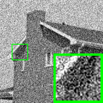 Figure 28
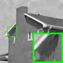 Figure 29
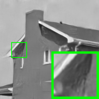 Figure 30
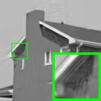 Figure 31
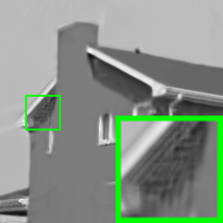 Figure 32
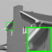 Figure 33
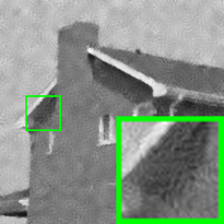 Figure 34
 Figure 35
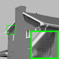 Figure 36
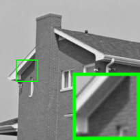 Figure 37
 Figure 38
 Figure 39
 Figure 40
| Noise std | 15 | 25 | 35 | 50 | 75 | ||||||||||
| Metric | PSNR | SSIM | PSNR | SSIM | PSNR | SSIM | PSNR | SSIM | PSNR | SSIM | |||||
| NLM [4] | 31.20 | 0.8483 | 28.64 | 0.7602 | 26.82 | 0.6762 | 24.80 | 0.5646 | 22.43 | 0.4224 | |||||
| BM3D [11] | 32.42 | 0.8860 | 30.02 | 0.8364 | 28.48 | 0.7969 | 26.85 | 0.7481 | 24.74 | 0.6649 | |||||
| LSSC [32] | 32.27 | 0.8849 | 29.84 | 0.8329 | 28.26 | 0.7908 | 26.64 | 0.7405 | 24.77 | 0.6746 | |||||
| NCSR [14] | 32.19 | 0.8814 | 29.76 | 0.8293 | 28.17 | 0.7855 | 26.55 | 0.7391 | 24.66 | 0.6793 | |||||
| WNNM [22] | 32.43 | 0.8841 | 30.05 | 0.8365 | 28.51 | 0.7958 | 26.92 | 0.7499 | 25.15 | 0.6903 | |||||
| TNRD [8] | 32.48 | 0.8845 | 30.07 | 0.8366 | 28.53 | 0.7957 | 26.95 | 0.7495 | 25.10 | 0.6901 | |||||
| DnCNN [59] | 32.59 | 0.8879 | 30.22 | 0.8415 | 28.66 | 0.8021 | 27.08 | 0.7563 | 25.24 | 0.6931 | |||||
| NLH (Blind) | 32.28 | 0.8796 | 30.09 | 0.8355 | 28.60 | 0.7988 | 27.11 | 0.7524 | 25.31 | 0.6932 | |||||
| Camera Settings | # | CBM3D | NI | NC | CC | MCWNNM | TWSC | DnCNN+ | FFDNet+ | CBDNet | NLH |
| Canon 5D M3 | 1 | 39.76 | 35.68 | 36.20 | 38.37 | 41.13 | 40.76 | 38.02 | 39.35 | 36.68 | 41.57 |
| ISO = 3200 | 2 | 36.40 | 34.03 | 34.35 | 35.37 | 37.28 | 36.02 | 35.87 | 36.99 | 35.58 | 37.39 |
| 3 | 36.37 | 32.63 | 33.10 | 34.91 | 36.52 | 34.99 | 35.51 | 36.50 | 35.27 | 36.68 | |
| Nikon D600 | 4 | 34.18 | 31.78 | 32.28 | 34.98 | 35.53 | 35.32 | 34.75 | 34.96 | 34.01 | 35.50 |
| ISO = 3200 | 5 | 35.07 | 35.16 | 35.34 | 35.95 | 37.02 | 37.10 | 35.28 | 36.70 | 35.19 | 37.21 |
| 6 | 37.13 | 39.98 | 40.51 | 41.15 | 39.56 | 40.90 | 37.43 | 40.94 | 39.80 | 41.34 | |
| Nikon D800 | 7 | 36.81 | 34.84 | 35.09 | 37.99 | 39.26 | 39.23 | 37.63 | 38.62 | 38.03 | 39.67 |
| ISO = 1600 | 8 | 37.76 | 38.42 | 38.65 | 40.36 | 41.43 | 41.90 | 38.79 | 41.45 | 40.40 | 42.66 |
| 9 | 37.51 | 35.79 | 35.85 | 38.30 | 39.55 | 39.06 | 37.07 | 38.76 | 36.86 | 40.04 | |
| Nikon D800 | 10 | 35.05 | 38.36 | 38.56 | 39.01 | 38.91 | 40.03 | 35.45 | 40.09 | 38.75 | 40.21 |
| ISO = 3200 | 11 | 34.07 | 35.53 | 35.76 | 36.75 | 37.41 | 36.89 | 35.43 | 37.57 | 36.52 | 37.30 |
| 12 | 34.42 | 40.05 | 40.59 | 39.06 | 39.39 | 41.49 | 34.98 | 41.10 | 38.42 | 42.02 | |
| Nikon D800 | 13 | 31.13 | 34.08 | 34.25 | 34.61 | 34.80 | 35.47 | 31.12 | 34.11 | 34.13 | 36.19 |
| ISO = 6400 | 14 | 31.22 | 32.13 | 32.38 | 33.21 | 33.95 | 34.05 | 31.93 | 33.64 | 33.45 | 34.70 |
| 15 | 30.97 | 31.52 | 31.76 | 33.22 | 33.94 | 33.88 | 31.79 | 33.68 | 33.45 | 34.83 | |
| Average | - | 35.19 | 35.33 | 35.65 | 36.88 | 37.71 | 37.81 | 35.40 | 37.63 | 36.44 | 38.49 |
| Camera Settings | # | CBM3D | NI | NC | CC | MCWNNM | TWSC | DnCNN+ | FFDNet+ | CBDNet | NLH |
| Canon 5D M3 | 1 | 0.9778 | 0.9600 | 0.9689 | 0.9678 | 0.9807 | 0.9805 | 0.9613 | 0.9723 | 0.9613 | 0.9847 |
| ISO = 3200 | 2 | 0.9552 | 0.9308 | 0.9427 | 0.9359 | 0.9591 | 0.9394 | 0.9415 | 0.9514 | 0.9430 | 0.9612 |
| 3 | 0.9660 | 0.9463 | 0.9476 | 0.9478 | 0.9676 | 0.9460 | 0.9553 | 0.9614 | 0.9562 | 0.9667 | |
| Nikon D600 | 4 | 0.9330 | 0.9413 | 0.9497 | 0.9484 | 0.9558 | 0.9581 | 0.9442 | 0.9506 | 0.9478 | 0.9606 |
| ISO = 3200 | 5 | 0.9168 | 0.9251 | 0.9398 | 0.9293 | 0.9534 | 0.9575 | 0.9187 | 0.9544 | 0.9406 | 0.9581 |
| 6 | 0.9313 | 0.9481 | 0.9588 | 0.9799 | 0.9684 | 0.9849 | 0.9278 | 0.9833 | 0.9751 | 0.9858 | |
| Nikon D800 | 7 | 0.9339 | 0.9506 | 0.9533 | 0.9575 | 0.9638 | 0.9671 | 0.9460 | 0.9590 | 0.9591 | 0.9709 |
| ISO = 1600 | 8 | 0.9383 | 0.9615 | 0.9591 | 0.9767 | 0.9683 | 0.9804 | 0.9547 | 0.9800 | 0.9781 | 0.9833 |
| 9 | 0.9277 | 0.9229 | 0.9406 | 0.9427 | 0.9537 | 0.9496 | 0.9170 | 0.9419 | 0.9183 | 0.9598 | |
| Nikon D800 | 10 | 0.8866 | 0.9101 | 0.9466 | 0.9637 | 0.9629 | 0.9770 | 0.8897 | 0.9755 | 0.9540 | 0.9750 |
| ISO = 3200 | 11 | 0.8928 | 0.9194 | 0.9309 | 0.9477 | 0.9510 | 0.9498 | 0.9221 | 0.9569 | 0.9476 | 0.9525 |
| 12 | 0.8430 | 0.9001 | 0.9070 | 0.9544 | 0.9578 | 0.9790 | 0.8563 | 0.9753 | 0.9492 | 0.9783 | |
| Nikon D800 | 13 | 0.7952 | 0.9074 | 0.9024 | 0.9206 | 0.9187 | 0.9369 | 0.7889 | 0.9140 | 0.9179 | 0.9436 |
| ISO = 6400 | 14 | 0.8613 | 0.8649 | 0.9141 | 0.9369 | 0.9379 | 0.9501 | 0.8844 | 0.9370 | 0.9290 | 0.9563 |
| 15 | 0.8363 | 0.8295 | 0.8847 | 0.9118 | 0.9225 | 0.9223 | 0.8637 | 0.9190 | 0.9121 | 0.9320 | |
| Average | - | 0.9063 | 0.9212 | 0.9364 | 0.9481 | 0.9548 | 0.9586 | 0.9115 | 0.9555 | 0.9460 | 0.9647 |
| Metric | CBM3D | NI | NC | MCWNNM | TWSC | DnCNN+ | FFDNet+ | CBDNet | NLH |
| PSNR | 34.51 | 35.11 | 35.43 | 37.38 | 37.96 | 37.90 | 37.61 | 38.06 | 38.81 |
| SSIM | 0.8507 | 0.8778 | 0.8841 | 0.9294 | 0.9416 | 0.9430 | 0.9415 | 0.9421 | 0.9520 |
| CPU (GPU) Time | 8.4 | 1.2 | 18.5 | 251.2 | 233.6 | 106.2 (0.05) | 49.9 (0.03) | 5.4 (0.40) | 5.3 |
| Aspect | Mean Image | Noisy Image |
| Patch-level NSS | 0.0043 | |
| Pixel-level NSS | 0.0026 |
| Value | 5 | 6 | 7 | 8 | Margin | |
| PSNR | 38.41 | 38.47 | 38.49 | 38.51 | 0.10 | |
| Value | 20 | 30 | 40 | 50 | Margin | |
| PSNR | 38.39 | 38.43 | 38.49 | 38.51 | 0.12 | |
| Value | 2 | 4 | 8 | 16 | Margin | |
| PSNR | 38.48 | 38.49 | 38.47 | 38.43 | 0.06 | |
| Value | 8 | 16 | 32 | 64 | Margin | |
| PSNR | 38.33 | 38.49 | 38.48 | 38.43 | 0.16 | |
| Value | 1.5 | 2 | 2.5 | 3 | Margin | |
| PSNR | 38.39 | 38.49 | 38.51 | 38.50 | 0.12 | |
| Value | 2 | 3 | 4 | 5 | Margin | |
| PSNR | 38.49 | 38.51 | 38.51 | 38.51 | 0.02 | |
| Value | 0.2 | 0.4 | 0.6 | 0.8 | Margin | |
| PSNR | 38.46 | 38.47 | 38.49 | 38.49 | 0.03 |
| Metric | NLH | Switch Columns | Switch Rows |
| PSNR | 38.49 | 31.08 | 38.49 |
| SSIM | 0.9647 | 0.8861 | 0.9647 |
Peer Reviews
No public reviews on file for this paper yet. If you reviewed it on a platform where reviews are public (OpenReview, ICLR, NeurIPS, ICML), you can paste yours below so the community can read it here.
Code & Models
Videos
No videos yet. Explain this paper in a talk, walkthrough, or lecture? Add one.
NLH: A Blind Pixel-level Non-local Method
for Real-world Image Denoising
Yingkun Hou, Member, IEEE, Jun Xu, Mingxia Liu, Guanghai Liu, Li Liu, Fan Zhu, Ling Shao
This work is supported by the National Natural Science Foundation of China (Grant No. 61379015, 61620106008 and 61866005). YK Hou is with School of Information Science and Technology, Taishan University, Tai’an, China. J Xu is with College of Computer Science, Nankai University, Tianjin, China. MX Liu is with School of Medicine, The University of North Carolina at Chapel Hill, USA. GH Liu is with School of Computer Science and Information Technology, Guangxi Normal University, China. L Liu, F Zhu and L Shao are with Inception Institute of Artificial Intelligence and Mohamed bin Zayed University of Artificial Intelligence, Abu Dhabi, UAE. J Xu ([email protected]) is the corresponding author.
Abstract
Non-local self similarity (NSS) is a powerful prior of natural images for image denoising. Most of existing denoising methods employ similar patches, which is a patch-level NSS prior. In this paper, we take one step forward by introducing a pixel-level NSS prior, i.e., searching similar pixels across a non-local region. This is motivated by the fact that finding closely similar pixels is more feasible than similar patches in natural images, which can be used to enhance image denoising performance. With the introduced pixel-level NSS prior, we propose an accurate noise level estimation method, and then develop a blind image denoising method based on the lifting Haar transform and Wiener filtering techniques. Experiments on benchmark datasets demonstrate that, the proposed method achieves much better performance than previous non-deep methods, and is still competitive with existing state-of-the-art deep learning based methods on real-world image denoising. The code is publicly available at https://github.com/njusthyk1972/NLH.
Index Terms:
Non-local self similarity, pixel-level similarity, image denoising.
I Introduction
Digital images are often subject to noise degradation during acquisition in imaging systems, due to the sensor characteristics and complex camera processing pipelines [36, 5, 35]. Removing the noise from the acquired images is an indispensable step for image quality enhancement in low-level vision tasks [19, 29, 50]. In general, image denoising aims to recover a clean image from its noisy observation , where is the corrupted noise. One popular assumption on is additive white Gaussian noise (AWGN) with standard deviation (std) . Recently, increasing attention has been paid to removing realistic noise, which is more complex than AWGN [53, 52, 54].
From the Bayesian perspective, image priors are of central importance for image denoising [28, 46, 47]. Numerous methods have been developed to exploit image priors for image denoising [57, 17, 48] and other image restoration tasks [42, 40, 41] over the past decades. These methods can be roughly divided into non-local self-similarity (NSS) based methods [4, 10, 27], sparsity or low-rankness based methods [16, 13, 22], dictionary learning based methods [18, 33, 32], generative learning based methods [43, 64, 37], and discriminative learning based methods [34, 59, 51], etc.
Among the above-mentioned methods, the NSS prior arises from the fact that, in a natural image, a local patch has many non-local similar patches across the image. Here, the similarity is often measured by Euclidean distance. The NSS prior has been successfully utilized by state-of-the-art image denoising methods, such as BM3D [10, 9, 11], WNNM [22], and N3Net [39], etc. However, most existing NSS-based methods [14, 13, 58] perform identical noise removal on similar but nuanced patches, which would results in artifacts. Despite its capability to enhance denoising performance, this patch-level NSS prior employed in these methods suffers from one major bottleneck. That is, it is very challenging to find closely similar patches for all the reference patches in a natural image, especially when the number of similar patches is large. To break through this bottleneck, the strategy of searching shape adaptive similar patches is proposed in BM3D-SAPCA [11]. Other improvements can also be found in [25]. However, this would introduce shape artifacts into the denoised image. Multi-scale techniques [62] have been proposed to enhance similarity, but the details would be degraded in the coarse scale and fail to detect similar counterparts.
In this work, we propose a pixel-level NSS prior for image denoising. The main idea of our work is illustrated in Figure 1. Our motivation is that, since pixel is the smallest component of natural images, by lifting from patch-level to pixel-level, the NSS prior can be utilized to a greater extent. We evaluate this point through an example on the commonly used “House” image (Figure 2 (a)). For each reference patch of size in “House”, we search its 16 most similar patches (including the reference patch itself) in the image by selecting the 16 minimum Euclidean distances which are computed between the reference patch and each patch in a neighborhood. We then compute the average value of these 16 Euclidean distances and further divide this average value by the number of pixels (i.e., 64) to obtain a pixel-wise distance . Here, the pixel-wise distance is defined as the distance apportioned to each pixel in this similar patch group which includes reference patch. We can see from Figures 2 (b) and (d) that the distance maps are all block like by the patch-level self-similarity measurement. In Figure 2 (b), we draw a histogram to show the relationship between the pixel-wise distance and the number of reference patches with given pixel-wise distance to their corresponding most similar patches. We observe that, less than reference patches (the darker bar) closely match their corresponding similar patches.
Then, we reshape each image patch in the similar patch group to 16 column vectors by column scanning and then stack them to form a matrix, further implement row matching also by Euclidean distance between a reference row and each of other rows in this matrix, in each row matching, we select 4 most similar rows (including the reference row itself) to form a similar pixel matrix, we average these 4 distances and further divide it by 64 to obtain the pixel-wise distance. We plot the histogram in Figure 2 (c) and one can see that the distance map value of each pixel by this method is different from others. We observe that, over reference patches contain closely matched pixels. Since Figure 2 (b) is the distance map between image patches, while Figure 2 (c) is the distance map between different rows of pixels. Since each set of similar patches contains 64 groups of similar pixel rows, the number of pixel distance maps are 64 times of the patch distance maps. Therefore, for the same image, the bin size in patch distance map (b) should be larger than that in the pixel distance map (c). We then add AWGN noise () to Figure 2 (a), compute the pixel-wise distances in patch-level NSS (as (b)) and pixel-level NSS (as (c)), and draw the histograms in Figures. 2 (d) and (e), respectively. We observe that, the histogram in Figure 2 (e) is shifted to left with a large margin, when compared to that in Figure 2 (d). All these results demonstrate that, the proposed pixel-level NSS can exploit the capability of NSS prior to a greater extent than previous patch-level NSS.
With the proposed pixel-level NSS prior, we develop an accurate noise level estimation method, and then propose a blind image denoising method based on non-local Haar (NLH) transform and Wiener filtering techniques. Experiments results show that, the proposed NLH method achieves much better performance than previous hand-crafted and non-deep methods, and is still competitive with existing state-of-the-art deep learning based methods on commonly tested real-world datasets. In summary, our contributions are manifold:
- •
We introduce a pixel-level NSS prior for image denoising, in which we find similar pixels instead of patches.
- •
With the pixel-level NSS prior, we propose an accurate noise level estimation method. Based on this, we propose a blind pixel-level image denoising method, and extend it for real-world image denoising.
- •
Extensive experiments on benchmark datasets demonstrate that, the proposed method achieves much better performance than previous non-deep methods, and is still competitive with existing state-of-the-art deep learning based methods on real-world image denoising.
The remainder of this paper is organized as follows. In §II, we briefly survey the related work. In §III, we present the proposed blind NLH method for image denoising. Extensive experiments are conducted in §IV to evaluate its noise level estimation performance, and compare it with state-of-the-art image denoising methods on both synthetic and realistic noise removal. Conclusion is given in §V.
II Related Work
Non-local Self Similarity (NSS): The NSS image prior is the essence to the success in texture synthesis [15], image denoising [10], super-resolution [20], and inpainting [3]. In the domain of image denoising, the NSS prior is firstly employed by the Non-local Means (NLM) method [4]. NLM estimates each pixel by computing a weighted average of all pixels in the image, where the weights are determined by the similarity between corresponding image patches centered at these pixels. Though this is a pixel-level method, NLM performs denoising based on the patch-level NSS prior. The patch-level NSS prior is l ater flourished in the BM3D method [10], and also in [57, 56, 55]. This prior performs denoising on groups of similar patches searched in non-local regions. These methods usually assume that the collected similar patches are fully matched. However, it is challenging to find closely similar patches for all the reference patches in a natural image. For more related work, please refer to [45]. In this work, instead of only searching similar patches, we propose to further search similar pixels and perform pixel-level denoising accordingly.
Real-world Image Denoising: Many real-world image denoising methods have been developed in the past decade [36, 56, 55]. The CBM3D method [9] first transforms an input RGB image into the luminance-chrominance space (e.g., YCbCr) and then applies the BM3D method [10] to each channel separately. The method of [30] introduces a “noise level function” to estimate the noise of the input image and then removes the noise accordingly. The methods of [26, 61] perform blind image denoising by estimating the noise level in image patches. The method of [36] employs a multivariate Gaussian to fit the noise in a noisy image and performs denoising accordingly. Neat Image [2] is a commercial software that removes noise according to the noise parameters estimated in a large enough flat region. MCWNNM [56] is a patch-level NSS prior based method, demanding a large number of similar patches for low-rank approximation. GCBD [7] is a blind image denoising method that uses the Generative Adversarial Network [21]. TWSC [55] introduces a weighting scheme into the sparse coding model [57] for real-world image denoising. It requires many similar patches for accurate weight calculation and denoising. Almost all these methods identically remove the noise in similar patches but ignore their internal variance. Besides, since the realistic noise in real-world images is pixel-dependent [36, 38, 1], patch-level NSS operations would generate artifacts when treating all the pixels alike. As such, real-world image denoising remains a very challenging problem [38, 1, 52].
III Proposed Blind Pixel-level Denoising Method
In this section, we present the proposed pixel-level Non-local Haar transform (NLH) based method for blind image denoising. The overall method includes three parts: 1) searching non-local similar pixels (§III-A), 2) noise level estimation (§III-B), and 3) a two-stage framework for image denoising (§III-C). The overall denoising framework is summarized in Figure 3. In the first stage, we employ the lifting Haar transform [44, 12] and bi-hard thresholding for local signal intensity estimation, which is later combined with the global noise level estimation for image denoising using Wiener filtering in the second stage. We then extend the proposed NLH method for real-world image denoising.
III-A Searching Non-local Similar Pixels
Given a gray-scale noisy image , we extract its local patches (assume there are totally patches). We stretch each local patch of size to a vector, denoted by (). For each , we search its most similar patches (including itself) by Euclidean distance in a large enough window (of size ) around it. We stack these vectors column by column (the patch with smaller distance is closer to the reference patch ) to form a noisy patch matrix .
To apply the NSS prior at the pixel-level, we further search similar pixels in by computing the Euclidean distances among the rows. Each row of contains pixels in the same relative position of different patches. The patch-level NSS prior guarantees that the pixels in the same row are similar to some extent. However, for rare textures and details, some pixels would suffer from large variance due to shape shifts. Processing these pixels identically would generate artifacts. To resolve this problem, we carefully select the pixels that are most similar to each other. Specifically, for the -th row of , we compute the distance between it and the -th row () as
[TABLE]
Note that for each row . We then select the ( is a power of ) rows, i.e., (, the row with smaller distance is closer to the reference row ), in with the smallest distances to , and finally aggregate the similar pixel rows as a matrix :
[TABLE]
where \{i_{1},...,i_{q}\}$$\subset$$\{1,...,n\}. The noisy pixel matrices () in the whole image are used for noise level estimation, which is described as follows.
III-B Noise Level Estimation
Accurate and fast estimation of noise levels is an essential step for efficient image denoising. The introduced pixel-level NSS prior can help achieve this goal. The rationale is that, since the pixels in the selected rows of are very similar to each other, the standard deviation (std) of among them can be viewed as the noise level. For simplicity, we assume that the noise follows a Gaussian distribution with std . Since the distances between the -th row of and its most similar rows are (), can be computed as
[TABLE]
Initial experiments indicate that the Eqn. (3) performs well for smooth areas, but is problematic for textures and structures. This is because, in these areas, the signal and noise are difficult to distinguish, and thus the noise level would be over-estimated. To make our method more robust for noise level estimation, we extend the noise level estimation from a local region to a global one. To do so, we estimate the local noise levels for all the noisy pixel matrices in the image, and simply set the global noise level as
[TABLE]
Discussion. The proposed pixel-based noise level estimation method assumes the noise in the selected rows follows a Gaussian distribution, which is consistent with the assumptions in [36, 55]. The proposed method is very simple, since it only computes the distances among the most similar pixels extracted from the image. As will be shown in the experimental section (§IV), the proposed noise level estimation method is very accurate, which makes it feasible to develop a blind image denoising method for real-world applications. Now we introduce the proposed two-stage denoising framework below.
III-C Two-stage Denoising Framework
The proposed denoising method consists of two stages. In the first stage, we estimate the local intensities via the non-local Haar (NLH) transform based bi-hard thresholding. With the results from the first stage, we perform blind image denoising by employing Wiener filtering based soft thresholding, in the second stage. Now, we introduce the two stages in details.
Stage 1: Local Intensity Estimation by Lifting Haar Transform based Bi-hard Thresholding. We have grouped a set of matrices () consisting of similar pixels. For simplicity, we ignore the index ) and estimate the global noise level . We perform denoising on the matrices consisting of similar pixels in the Haar transformed domain [24]. Here, we utilize the lifting Haar wavelet transform (LHWT) [44, 12] due to its flexible operation, faster speed, and lightweight memory.
The LHWT matrices we employ here are two orthogonal matrices and . We set as powers of to accommodate the noisy pixel matrices with the Haar transform. The LHWT transform of the non-local similar pixel matrix , i.e., the matrix consist of similar pixels is to obtain the transformed noisy coefficient matrix via
[TABLE]
Due to limited space, we put the detailed LHWT transforms with specific in the Appendix.
After LHWT transforms, we restore the -th () element in -th row () of the noisy coefficient matrix via hard thresholding:
[TABLE]
where means element-wise production, is the indicator function, and is the threshold parameter. According to the wavelet theory [44], the coefficients in the last two rows of (except the -st column) are in the high frequency bands of the LHWT transform, which should largely be noise. To remove this noise in , we introduce a structurally hard thresholding strategy and completely set to [math] all the coefficients in the high frequency bands of :
[TABLE]
where and are the -th entry of the coefficient matrices and , respectively. We then employ inverse LHWT transforms [44, 12] on to obtain the denoised pixel matrix via
[TABLE]
where and are inverse LHWT matrices. Detailed inverse LHWT with specific are put in the Appendix. Finally, we aggregate all the denoised pixel matrices to form the denoised image. The elements in can be viewed as local signal intensities, which are used in Stage 2 for precise denoising with the globally estimated noise level . To obtain more accurate estimation of local signal intensities, we perform the above LHWT transform based bi-hard thresholding for iterations. For the -th () iteration, we add the denoised image back to the original noisy image and obtain the noisy image as
[TABLE]
Stage 2: Blind Denoising by Iterative Wiener Filtering. The denoised image in the Stage 1 is only a basic estimation of the latent clean image, and it is taken as a reference image for further fine-grained denoising in this stage via Wiener filtering. In order to remove the noise more clear while preserving the details, we employ the Wiener filtering based soft thresholding for finer denoising. We use the above estimated local signal intensities and the globally estimated noise level to perform Wiener filtering on the coefficients obtained by the LHWT transform of the original noisy pixel matrices. To further improve the denoising performance, in all experiments, we conduct the Wiener filtering based soft thresholding for two iterations. In the first iteration, we perform Wiener filtering on in Eqn. (5) as
[TABLE]
and then we perform the second Wiener filtering as
[TABLE]
Note that both the original noisy image and the roughly denoised image are required in the Stage 2. Just as shown by Eqns. (10) and (11), to perform Wiener filtering, we need the Haar transformed coefficients of both the original noisy image and the roughly denoised image in the Stage 2. To this end, we need simultaneously transform the matrix of similar pixels from the original noisy image, and that of the denoised image obtained in the Stage 1, to implement the Wiener filtering in the Stage 2 of our NLH. Experiments on image denoising demonstrate that, the proposed method with two iterations performs the best, while using more iterations brings little improvement. We then perform inverse LHWT transforms (please see details in the Appendix) on to obtain the denoised pixel matrix . Finally, we aggregate all the denoised pixel matrices to form the final denoised image.
III-D Complexity Analysis
The proposed NLH contains three parts: 1) In §III-A, the complexity of searching similar patches is , while the complexity of searching similar pixels is . Since we set , the overall complexity is . 2) In §III-B, the complexity for noise level estimation is , which can be ignored. 3) In §III-C, the complexity of the two stages are and , respectively. Since we have , the complexity of NLH is .
III-E Extension to Real-world Image Denoising
To accommodate the proposed NLH method with real-world RGB images, we first transform the RGB images into the luminance-chrominance (e.g., YCbCr) space [10], and then perform similar pixel searching in the Y channel. The similar pixels in the other two channels (i.e., Cb and Cr) are correspondingly grouped. We perform denoising for each channel separately and aggregate the denoised channels back to form the denoised YCbCr image. Finally, we transform it back to the RGB space for visualization.
IV Experiments and Results
In this section, we first evaluate the developed noise level estimation method on synthetic noisy images. The goal is to validate the effectiveness of our pixel-level non-local self similarity (NSS) prior. We then evaluate the proposed NLH method on both synthetic images corrupted by additive white Gaussian noise (AWGN) and real-world noisy images. Finally, we perform comprehensive ablation studies to gain a deeper insight into the proposed NLH method. More results on visual quality can be found in the Supplementary File.
IV-A Implementation Details
The proposed NLH method has 7 main parameters: patch size , window size for searching similar patches, number of similar patches , number of similar pixels , regularization parameter , hard threshold parameter , and iteration number (, , only exist in Stage 1). In all experiments, we set , , , , . For synthetic AWGN corrupted image denoising, we set for , for in both stages. For real-world image denoising, we set , in both stages.
IV-B Results on Noise Level Estimation
The proposed pixel-level NSS prior can be used to estimate the noise level of the input noisy image. We compare our method (Eqn. (4)) with leading noise level estimation methods, such as Zoran et al. [63], Liu et al. [31], and Chen et al. [6]. The comparison is performed on the 68 images from the commonly tested BSD68 dataset. We generate synthetic noisy images by adding AWGN with \sigma$$\in$$\{5,15,25,35,50,75,100\} to the clean images. The comparison results are listed in Table I. The presented noise levels of different methods are averaged on the whole dataset. One can see that, the proposed method can accurately estimate different noise levels for various noisy images. Note that the proposed method only utilizes the introduced pixel-level NSS prior, and the results indeed validate its effectiveness on noise level estimation.
IV-C
Results on Synthetic AWGN Corrupted Images
On 20 gray-scale images (listed in Figure 4) widely used in [10, 22, 57], we compare the proposed NLH method with several competing AWGN denoising methods, such as BM3D [10], LSSC [32], NCSR [14], WNNM [22], TNRD [8], and DnCNN [59]. For BM3D, we employ its extension called BM3D-SAPCA [11], which usually performs better than BM3D on gray-scale images. We employ the Non-Local Means (NLM) [4] as a baseline to validate the effectiveness of the pixel-level NSS prior. The source codes of these methods are downloaded from the corresponding authors’ websites, and we use the default parameter settings. The methods of TNRD and DnCNN are discriminative learning based methods, and we use the models trained originally by their authors. The noisy image is generated by adding AWGN noise with standard deviation (std) to the corresponding clean image, and in this paper we set . Note that the noise level is the same for each image of the whole dataset.
From Table II we can see that, the proposed NLH is comparable with the leading denoising methods on average PSNR (dB) and SSIM [49]. Note that TNRD and DnCNN are trained on clean and synthetic noisy image pairs, while NLH can blindly remove the noise with the introduced pixel-level NSS prior. By comparing the performance of NLM and NLH, one can see that the proposed pixel-level denoising method performs much better than simply averaging the central pixels of similar patches. The visual quality comparisons can be found in Figure 6. We observe that our NLH produces more visual pleasing results than the other methods.
IV-D Results on Real-World Noisy Images
Comparison methods. We compare the proposed NLH method with CBM3D [9], a commercial software Neat Image (NI) [2], “Noise Clinic” (NC) [26], Cross-Channel (CC) [36], MCWNNM [56], TWSC [55]. CBM3D can directly deal with color images, and the std of input noise is estimated by [6]. For MCWNNM and TWSC, we use [6] to estimate the noise std () for each channel and perform denoising accordingly. We also compare the proposed NLH method with DnCNN+ [59], FFDNet+ [60] and CBDNet [23], which are state-of-the-art convolutional neural network (CNN) based image denoising methods. FFDNet+ is a multi-scale extension of FFDNet [60] with a manually selected uniform noise level map. DnCNN+ is based on the color version of DnCNN [59] for blind denoising, but fine-tuned with the results of FFDNet+ [60]. Note that for FFDNet+ and DnCNN+, there is no need to estimate the noise std. For the three CNN based methods, we asked the authors to run the experiments for us. We also run the codes using our machine for speed comparisons.
Datasets and Results. We evaluate our NLH on two benchmark datasets on real-world image denoising, i.e., the Cross-Channel (CC) dataset [36] and the Darmstadt Noise Dataset (DND) [38].
The CC dataset [36] includes noisy images of 11 static scenes captured by Canon 5D Mark 3, Nikon D600, and Nikon D800 cameras. The real-world noisy images were collected under a controlled indoor environment. Each scene is shot 500 times using the same camera and settings. The average of the 500 shots is taken as the “ground truth”. The authors cropped 15 images of size to evaluate different denoising methods, as shown in Figure 5. The comparisons in terms of PSNR and SSIM are listed in Table III and Table IV, respectively. It can be seen that, the proposed NLH method achieves the highest results on most images. Figure 7 shows the denoised images yielded by different methods on a scene captured by a Nikon D800 with ISO=1600. As can be seen, NLH also achieves better visual quality than other methods.
The DND dataset [38] includes 50 different scenes captured by Sony A7R, Olympus E-M10, Sony RX100 IV, and Huawei Nexus 6P. Each scene contains a pair of noisy and “ground truth” clean images. The noisy images are collected under higher ISO values with shorter exposure times, while the “ground truth” images are captured under lower ISO values with adjusted longer exposure times. For each scene, the authors cropped 20 bounding boxes of size , generating a total of 1000 test crops. The “ground truth” images are not released, but we can evaluate the performance by submitting the denoised images to the DND’s Website. In Table V, we list the average PSNR (dB) and SSIM [49] results of different methods. Figure 8 shows the visual comparisons on the image “0001_18” captured by a Nexus 6P camera. It can be seen that, the proposed NLH achieves higher PSNR and SSIM results, with better visual quality, than the other methods.
Speed. We also compare the speed of all competing methods. All experiments are run under the Matlab 2016a environment on a machine with a quad-core 3.4GHz CPU and 8GB RAM. We also run DnCNN+, FFDNet+, and CBDNet on a Titan XP GPU. In Table V, we also show the average run time (in seconds) of different methods, on the 1000 RGB images of size in [38]. The fastest result is highlighted in bold. It can be seen that, Neat Image only needs an average of 1.2 seconds to process a RGB image. The proposed NLH method needs seconds (using parallel computing), which is much faster than the other methods, including the patch-level NSS based methods such as MCWNNM and TWSC, the CNN based methods DnCNN+, FFDNet+, and CBDNet. The majority of time in the proposed NLH method is spent on searching similar patches, which takes an average of 2.8 seconds. Further searching similar pixels only takes an average of 0.3 seconds. This demonstrates that, the introduced pixel-level NSS prior adds only a small amount of calculation, when compared to its patch-level counterpart.
Discussion. Our NLH achieves slightly improved results for gray-scale noisy image corrupted by AWGN noise, but is dramatically better on real-world noisy images when compared to the other methods [10], including the deep learning based methods [59, 23]. One the authors provide some kind of intuition on why the method our proposed non-local similar pixel searching scheme is feasible to transform the realistic noise, which is not Gaussian distributed [19, 38, 55] to the quasi-Gaussian noise. To validate this point, we perform patch matching (block matching) followed by pixel matching (row matching) in a real-world noisy image from the CC dataset [36]. This process is illustrated in Figure 9. We add = 5 Gaussian noise to the mean image (clean image) in CC dataset, then implement block matching and row matching to obtain a similar pixels group which can be seen in Figure 9 (a), and we give the red channel noise histogram of the similar pixels group in Figure 9 (b). On the other hand, we directly implement block matching and row patching on the real world image in Figure 9 (c) and give its red channel noise histogram of similar pixels group in Figure 9 (d). Because the signal-dependent noise color is mainly red, so comparing red channel histogram is much objective. We can see in two histograms that the noise value in two similar pixels groups are almost equal, this is the reason of adding = 5 Gaussian noise. We observe that the realistic noise in Figure 9 (c), which is usually not Gaussian distributed in images patches, is signal-dependent and can hardly be separated from the image patches. However, our proposed NLH is able to transform the signal dependent realistic noise to quasi-Gaussian noise. This ability of transforming realistic noise to quasi-Gaussian one makes our NLH very effective for realistic noise removal over previous image denoising methods, which are original designed for Gaussian noise removal or trained on the realistic noise different with the test ones. This is the key reason that why our NLH achieves dramatically better denoising performance on real-world noisy images, but similar performance on Gaussian noisy images, when compared to deep learning based approaches like DnCNN [59].
IV-E Validation of the Proposed NLH Method
We conduct more detailed examinations of our NLH to assess 1) the accuracy of pixel-level NSS vs. patch-level NSS; 2) the contribution of the proposed pixel-level NSS prior for NLH on real-world image denoising; 3) the necessity of the two-stage framework; and 4) the individual influence of the 7 major parameters on NLH; 5) is the proposed noise estimation method or the proposed denoising algorithm contributes to the improvement of PSNR? 6) How the order of columns (or rows) influences our NLH on image denoising?
1. Is pixel-level NSS more accurate than patch-level NSS? To answer this question, we compute the average pixel-wise distances (APDs, the distance apportioned to each pixel) of non-local similar pixels and patches on the CC dataset [36]. From Table VI, we can see that, on 15 mean images and 15 noisy images (normalized into ), the APDs of pixel-level NSS are smaller than those of patch-level NSS. In other words, pixel-level NSS is more accurate than the patch-level NSS on similarity measurements.
2. Does pixel-level NSS prior contribute to image denoising? Here, we study the contribution of the proposed pixel-level NSS prior. To this end, we remove the searching of pixel-level NSS in NLH. Thus we have a baseline: w/o Pixel NSS. From Table VII, we observe a clear drop in PSNR (dB) and SSIM results over two datasets, which implies the effectiveness of the proposed pixel-level NSS prior.
3. Is Stage 2 necessary? We also study the effect of the Stage 2 in NLH. To do so, we remove the Stage 2 from NLH, and have a baseline: w/o Stage 2. From Table VII, we can see a huge performance drop on two datasets. This shows that, the Stage 2 complements the Stage 1 with soft Wiener filtering, and is essential to the proposed NLH.
4. How each parameter influences NLH’s denoising performance? The proposed NLH mainly has 7 parameters (please see §IV-A for details). We change one parameter at a time to assess its individual influence on NLH. Table VIII lists the average PSNR results of NLH with different parameter values on CC dataset [36]. It can be seen that: 1) The variations of PSNR results are from 0.02dB (for iteration number ) to 0.16dB (for number of similar patches ), when changing individual parameters; 2) The performance on PSNR increases with increasing patch size , window size , or iteration number . For performance-speed tradeoff, we set \sqrt{n}$$=$$7, W$$=$$40, and K$$=$$2 in NLH for efficient image denoising; 3) The number of similar pixels is novel in NLH. To our surprise, even with q$$=$$2 similar pixels, NLH still performs very well, only drop 0.01dB on PSNR compared to case with q$$=$$4. However, with q$$=$$8,, the performance of NLH decreases gradually. The reason is that, searching more (e.g., ) pixels in 7$$\times$$7 patches may decrease the accuracy of pixel-level NSS, hence degrade the performance of NLH. Similar trends can be observed by changing the number of similar patches, i.e., the value of . In summary, all the parametric analyses demonstrate that, NLH is very robust on real-world image denoising, as long as the 7 parameters are set in reasonable ranges.
5. Is the proposed noise estimation method or the proposed denoising algorithm contributes to the improvement of the PSNR? To anwser this question, we performed essential real-world image denoising experiments on the CC [36] dataset for the comparison methods such as CBM3D [9], MCWNNM [56], and TWSC [55], using our proposed noise estimation method (Eqn. (4)). The PSNR and SSIM [49] results of these methods on the CC dataset are provided in Tables IX. We observe that, by using our proposed noise estimator, all these methods are improved with better denoising results on the CC dataset. However, even with the improvements, these methods still have a performance gap when compared with our NLH. This shows that accurate noise estimation is helpful, but not the most important component for state-of-the-art performance on image denoising. These results also demonstrate that the improvements of the denoising results by our NLH is not mainly from the proposed noise estimator, but is from the NLH denoising method itself.
- How the order of columns (or rows) influences our NLH on image denoising? To study this problem, we proposed two variants of the original NLH. The first variant is named “Switch Columns”: for each similar patch matrix, we switch the reference patch (the first column) with its least similar column (the last column), while keeping the order of rows fixed. The second variant is named “Switch Rows”: for each similar pixel matrix, we switch the reference row in the first row with the least similar row in the last row, while keeping the order of columns fixed. As show in Table X, on the the CC dataset [36], the variant of “Switch Rows” achieves close PSNR and SSIM [49] results with those of the original NLH. However, the variant of “Switch Column” suffers from significant performance drop when compared to the original NLH. The key lies on the number of similar columns (or rows) in each similar patch (or pixel) matrix. On one hand, the number of similar rows in our NLH is small (4 in stage one and 8 in stage two). Thus in most cases the rows of pixels could be very similar to each other, and switching the rows does not influence little on the final results. On the other, the number of similar patches is relatively large (16 in stage one and 64 in stage two) to exploit the non-local self similar property of natural images. Therefore, it is likely that some patches are not that similar to the reference one. Then, if we switch the reference patch in the first column with the least similar patch in the last column, the denoising results degrade significantly.
V Conclusion
How to utilize the non-local self similarity (NSS) prior for image denoising is an open problem. In this paper, we attempted to utilize the NSS prior to a greater extent by lifting the patch-level NSS prior to the pixel-level NSS prior. With the pixel-level NSS prior, we developed an accurate noise level estimation method, based on which we proposed a blind image denoising method. We estimated the local signal intensities via non-local Haar (NLH) transform based bi-hard thresholding, and performed denoising accordingly by Wiener filtering based soft thresholding. Experiments on benchmark datasets demonstrated that, the proposed NLH method significantly outperforms previous hand-crafted and non-deep methods, and is still competitive with existing state-of-the-art deep learning based methods on real-world image denoising task. We will simplify the pipeline of our NLH in the future work.
VI Appendix: Detailed horizontal/vertical LHWT transforms and their inverse transforms
The Haar transform in our NLH is used differently from the traditional Haar transform on images. The reasons are: 1) in our NLH the matrices of similar pixels for Haar transform are not square ones, while traditional Haar transform needs square images; 2) these matrices of similar pixels are relatively small. Therefore, traditional orthogonal Haar transform used on image-level transform is not suitable for the small matrix-level scenarios in the proposed NLH. We employ an alternative lifting Haar transform, which is adaptive to our NLH.
For each row in the noisy patch matrix , we select the () rows, i.e., (), in with the smallest Euclidean distances to , and stack the similar pixel rows as a matrix . can also be written column by column as , where contains selected rows in (). For simplicity, we ignore the indices and have . is written as , and is written as (). Hence, can be written column by column as , where contains selected rows in ().
The proposed NLH contains horizontal and vertical LHWT transforms. For both stages, we set , in all experiments. We first perform a horizontal LHWT transform (i.e., as described in Eqn. (5) in the main paper):
[TABLE]
We stack the coefficient vectors together and form . Assume that is the -th row of , i.e., , we then perform vertical LHWT transform (i.e., as described in Eqn. (5) in the main paper):
[TABLE]
Then we perform a trivial hard thresholding operation:
[TABLE]
where means element-wise production, is the indicator function, and is the threshold parameter. We also perform a structurally hard thresholding and completely set to [math] all the coefficients in the high frequency bands of :
[TABLE]
where is the -th entry of the coefficient matrices , respectively.
After the two hard thresholding steps, we perform inverse vertical and horizontal LHWT transforms. For simplicity, we still use the definitions in Eqn. (13). We first perform an inverse vertical LHWT transform (i.e., as described in Eqn. (8)):
[TABLE]
We stack the rows of coefficients () together and form a matrix . Assume that is the -th column of , i.e., , we then perform an inverse horizontal LHWT transform (i.e., as described in Eqn. (8)):
[TABLE]
[TABLE]
We stack together and form the denoised pixel matrix in the first stage. We then aggregate all the denoised pixel matrices to form the denoised image. In the first stage, we perform the LHWT and inverse LHWT transforms for iterations. Note that we employ standard LHWT transforms without any modification.
The reference list from the paper itself. Each links out to its DOI / PubMed record.
- 1[1] A. Abdelhamed, S. Lin, and M. S. Brown. A high-quality denoising dataset for smartphone cameras. In IEEE Conference on Computer Vision and Pattern Recognition (CVPR) , June 2018.
- 2[2] N. AB Soft. Neat Image. https://ni.neatvideo.com/home .
- 3[3] C. Barnes, E. Shechtman, A. Finkelstein, and D. Goldman. Patchmatch: A randomized correspondence algorithm for structural image editing. ACM Transactions on Graphics , 28(3):24, 2009.
- 4[4] A. Buades, B. Coll, and J. M. Morel. A non-local algorithm for image denoising. In IEEE Conference on Computer Vision and Pattern Recognition (CVPR) , pages 60–65, 2005.
- 5[5] C. Chen, Q. Chen, J. Xu, and V. Koltun. Learning to see in the dark. In IEEE Conference on Computer Vision and Pattern Recognition (CVPR) , 2018.
- 6[6] G. Chen, F. Zhu, and A. H. Pheng. An efficient statistical method for image noise level estimation. In IEEE International Conference on Computer Vision (ICCV) , 2015.
- 7[7] J. Chen, J. Chen, H. Chao, and M. Yang. Image blind denoising with generative adversarial network based noise modeling. In IEEE Conference on Computer Vision and Pattern Recognition (CVPR) , pages 3155–3164, 2018.
- 8[8] Y. Chen and T. Pock. Trainable nonlinear reaction diffusion: A flexible framework for fast and effective image restoration. IEEE Transactions on Pattern Analysis and Machine Intelligence , 39(6):1256–1272, 2017.
