Impact of Stellar Superflares on Planetary Habitability
Yosuke A. Yamashiki, Hiroyuki Maehara, Vladimir Airapetian, Yuta, Notsu, Tatsuhiko Sato, Shota Notsu, Ryusuke Kuroki, Keiya Murashima, Hiroaki, Sato, Kosuke Namekata, Takanori Sasaki, Thomas B. Scott, Hina Bando, Subaru, Nashimoto, Fuka Takagi, Cassandra Ling, Daisaku Nogami

TL;DR
This study quantitatively evaluates how stellar superflares and associated radiation impact the habitability of exoplanets, considering atmospheric effects and flare frequency, with implications for planets like Proxima Centauri b and TRAPPIST-1 e.
Contribution
First to develop a quantitative impact evaluation system for stellar flares on exoplanet habitability, focusing on ionizing radiation effects and atmospheric escape.
Findings
Ground-level radiation doses are below critical for complex life at 1 bar atmosphere.
Maximum stellar flares can cause fatal radiation doses on some exoplanets.
High XUV flux induces significant atmospheric escape, reducing habitability potential.
Abstract
High-energy radiation caused by exoplanetary space weather events from planet-hosting stars can play a crucial role in conditions promoting or destroying habitability in addition to the conventional factors. In this paper, we present the first quantitative impact evaluation system of stellar flares on the habitability factors with an emphasis on the impact of Stellar Proton Events. We derive the maximum flare energy from stellar starspot sizes and examine the impacts of flare associated ionizing radiation on CO, H, N+O --rich atmospheres of a number of well-characterized terrestrial type exoplanets. Our simulations based on the Particle and Heavy Ion Transport code System [PHITS] suggest that the estimated ground level dose for each planet in the case of terrestrial-level atmospheric pressure (1 bar) for each exoplanet does not exceed the critical dose for complex…
Click any figure to enlarge with its caption.
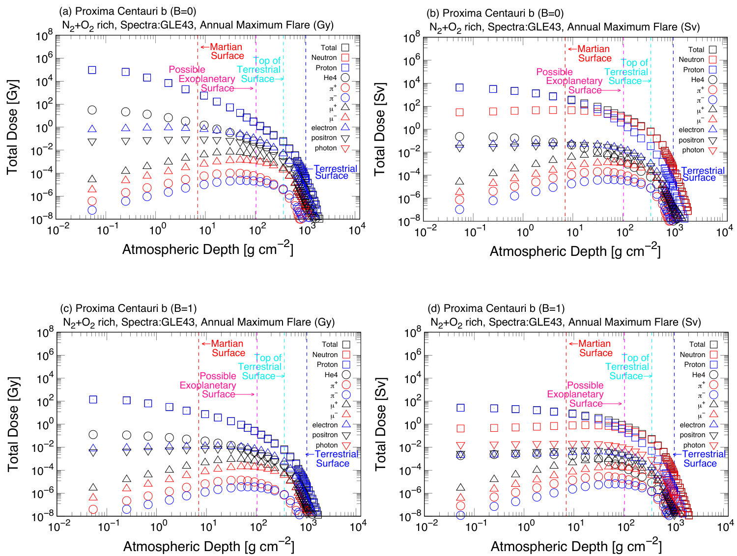 Figure 1
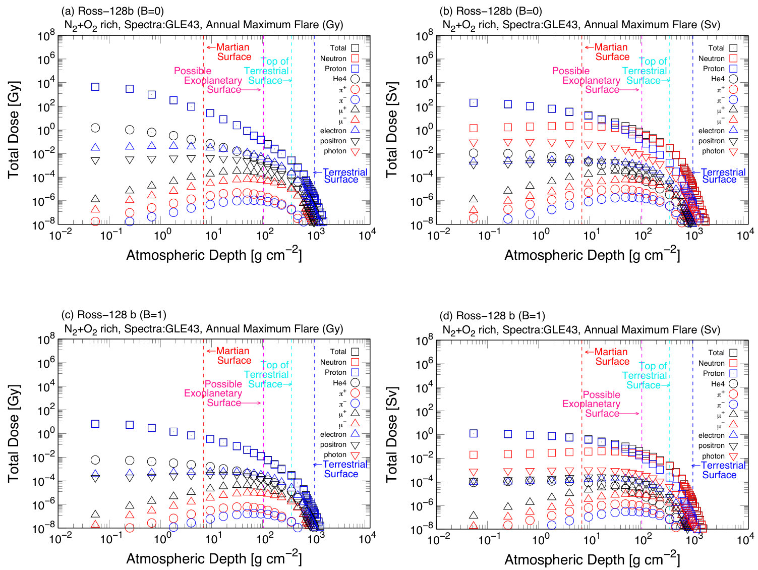 Figure 2
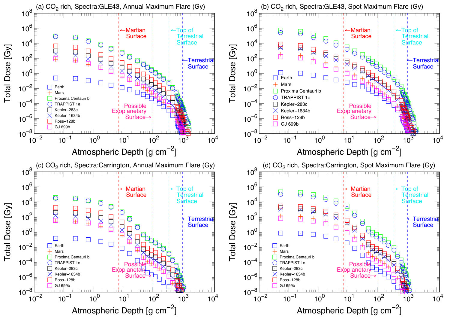 Figure 3
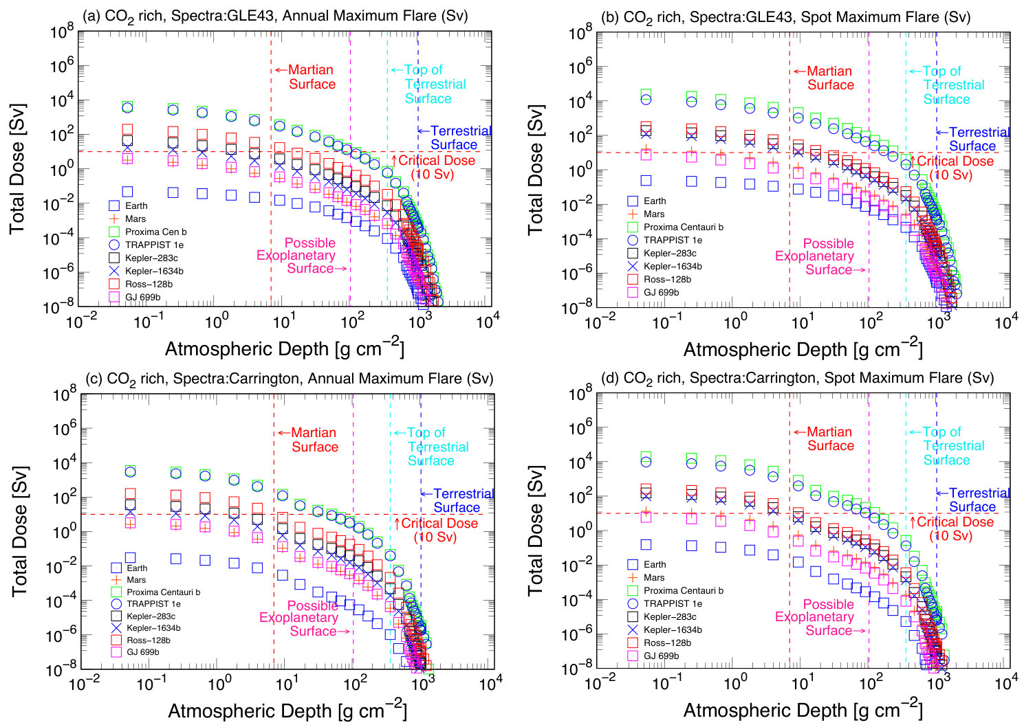 Figure 4
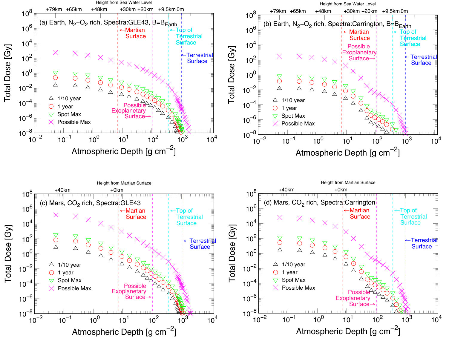 Figure 5
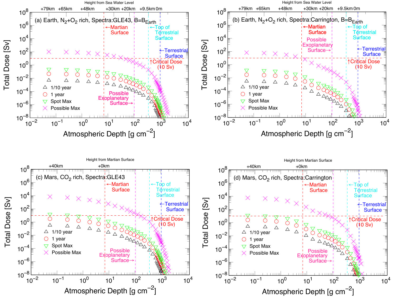 Figure 6
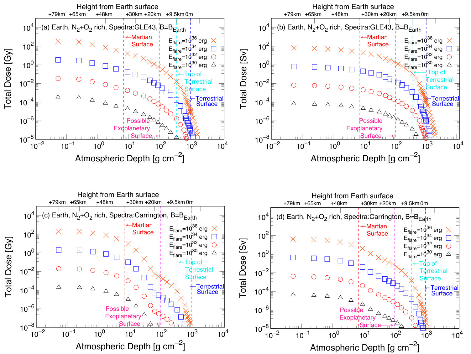 Figure 7
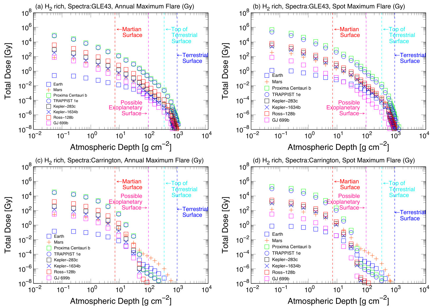 Figure 8
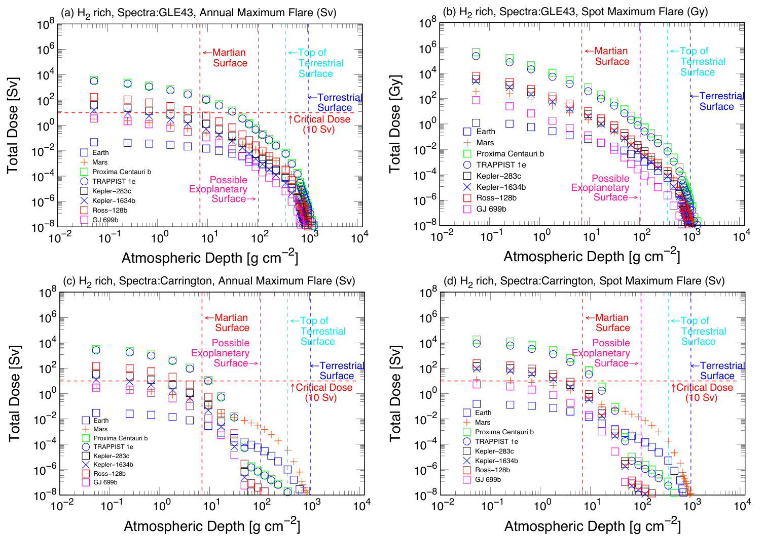 Figure 9
 Figure 10
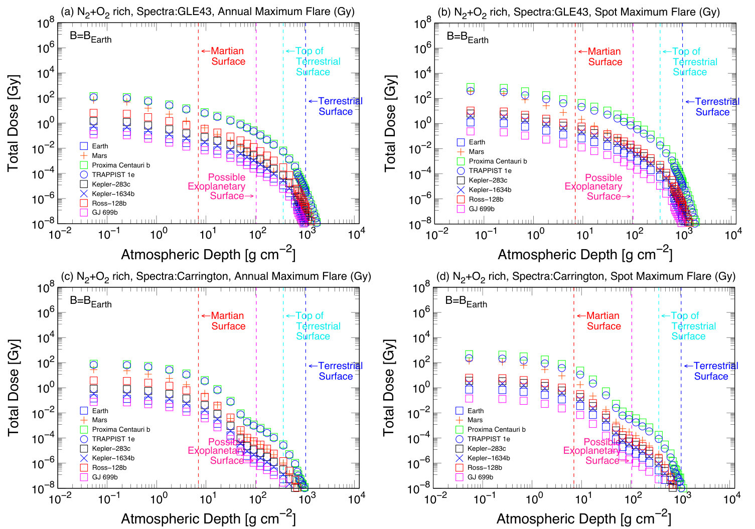 Figure 11
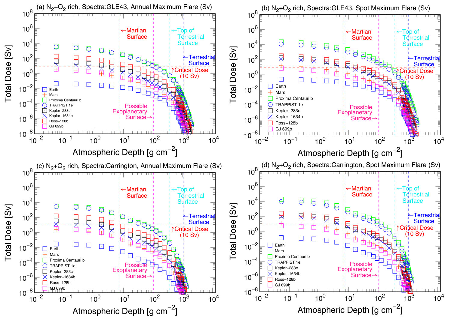 Figure 12
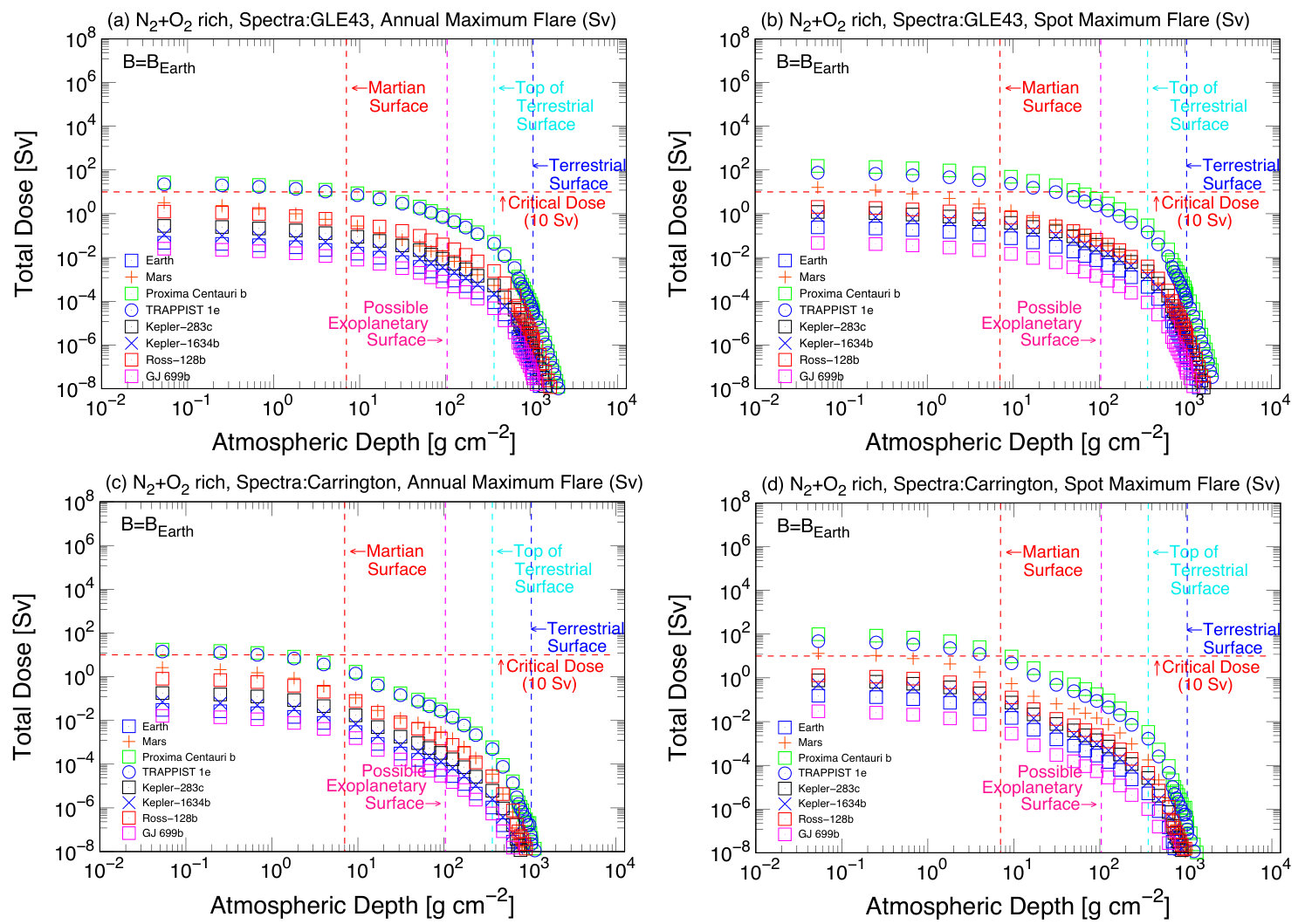 Figure 13
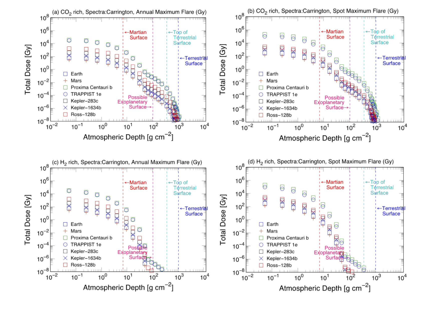 Figure 14
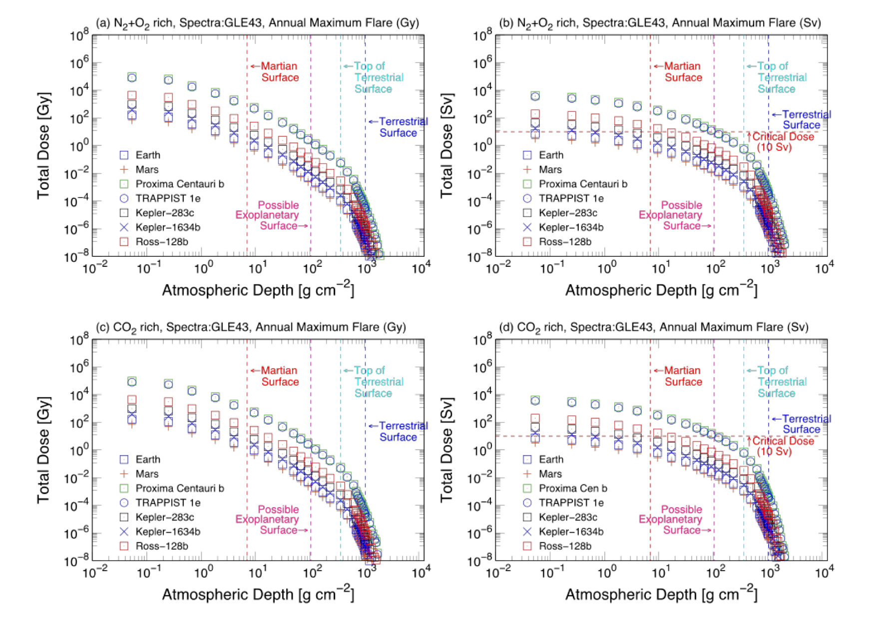 Figure 15
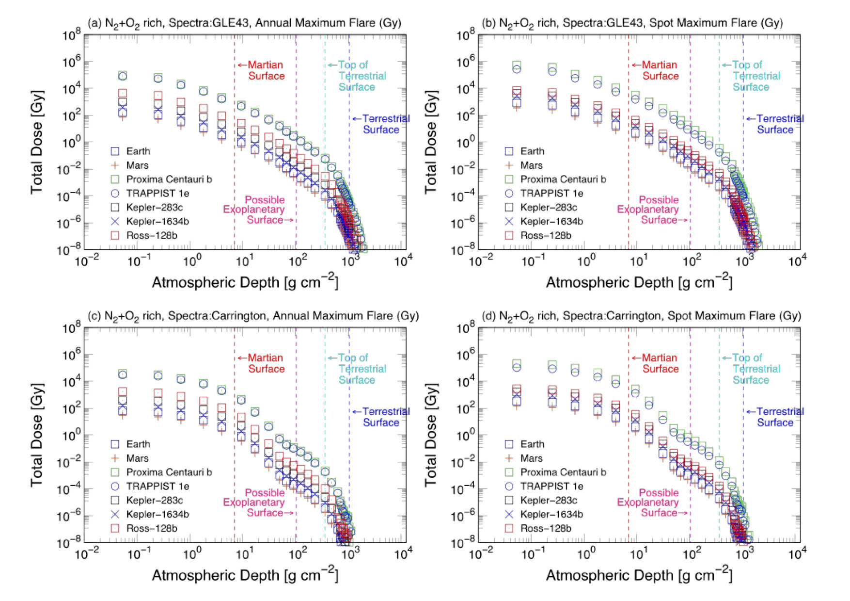 Figure 16
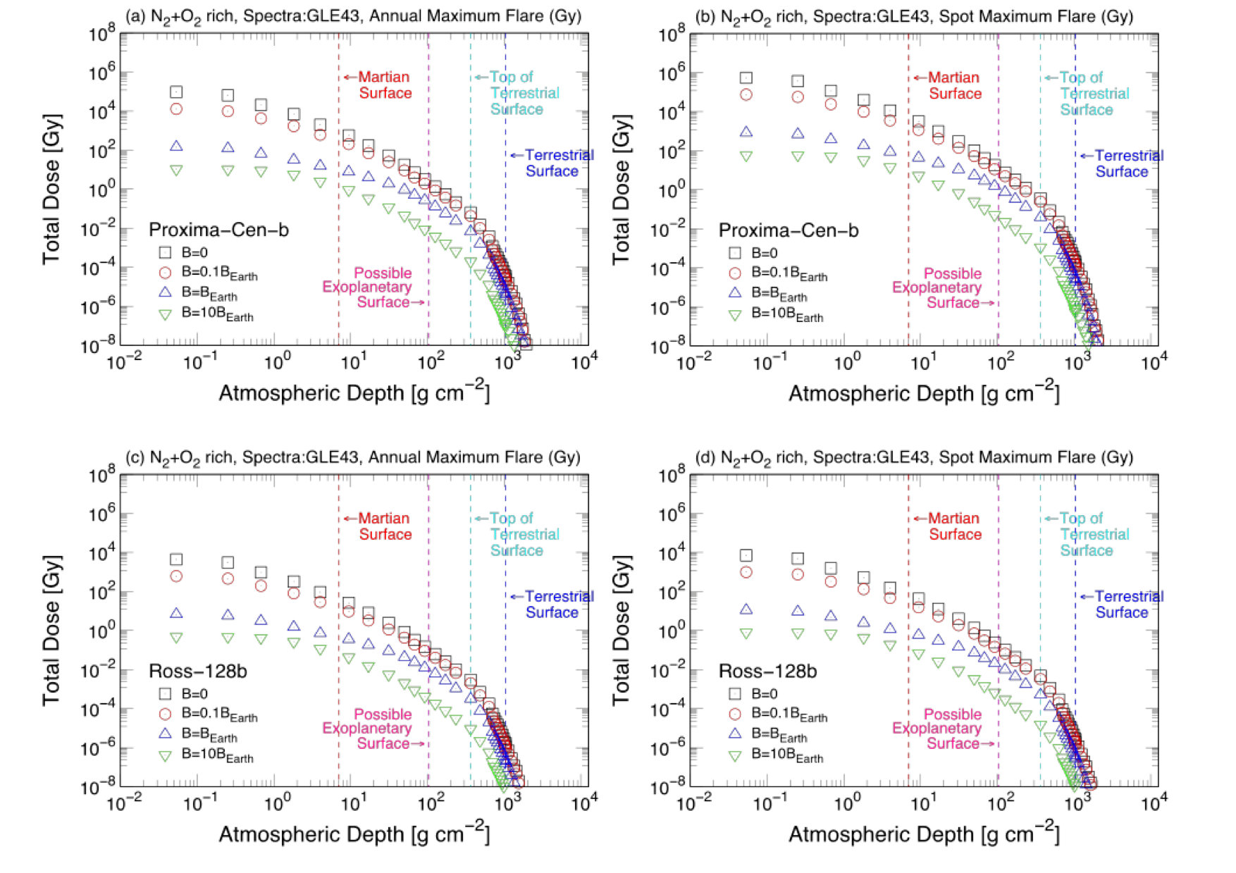 Figure 17
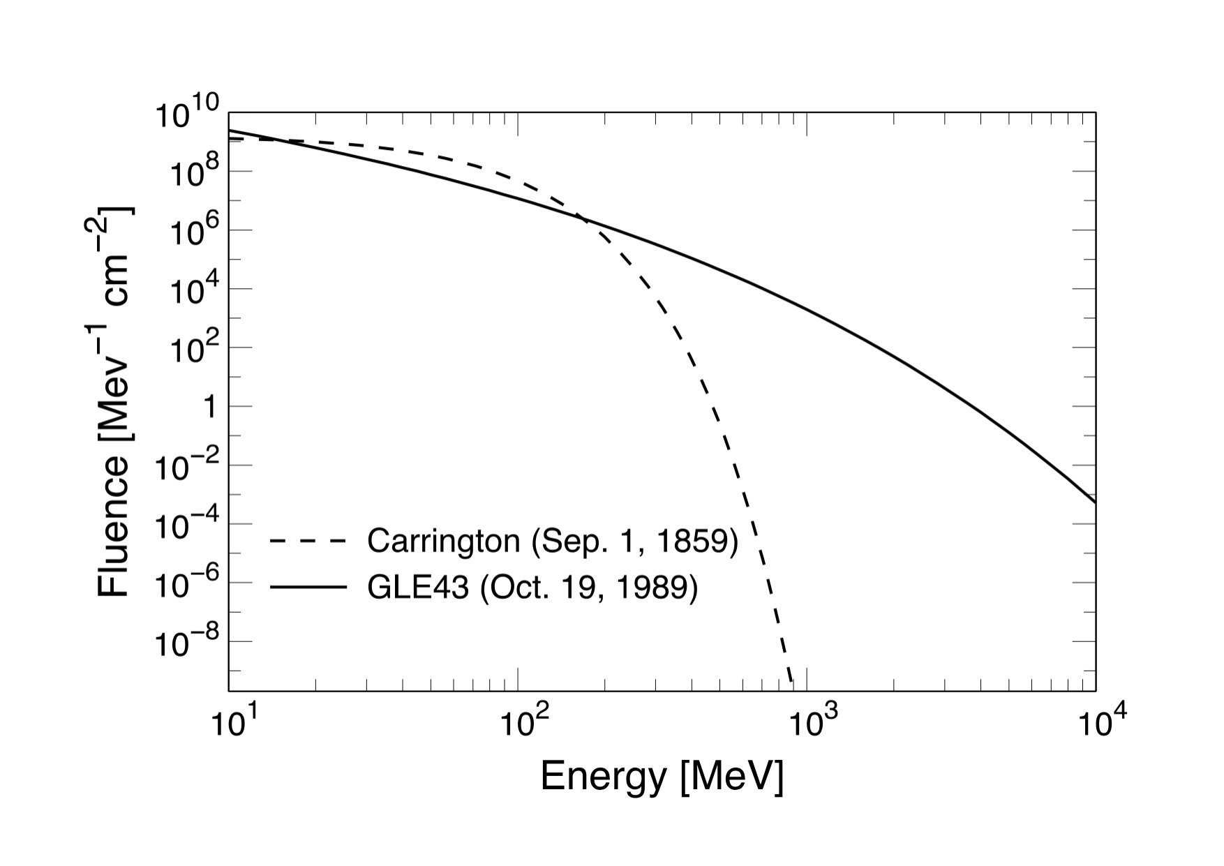 Figure 18
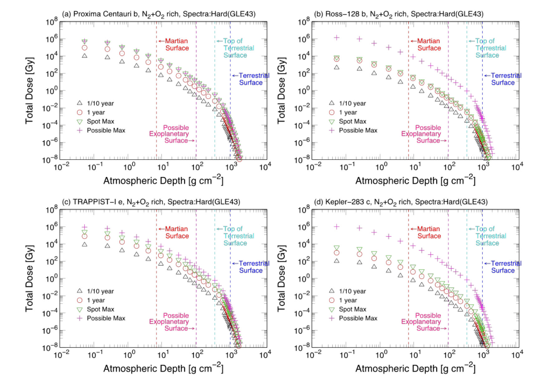 Figure 19
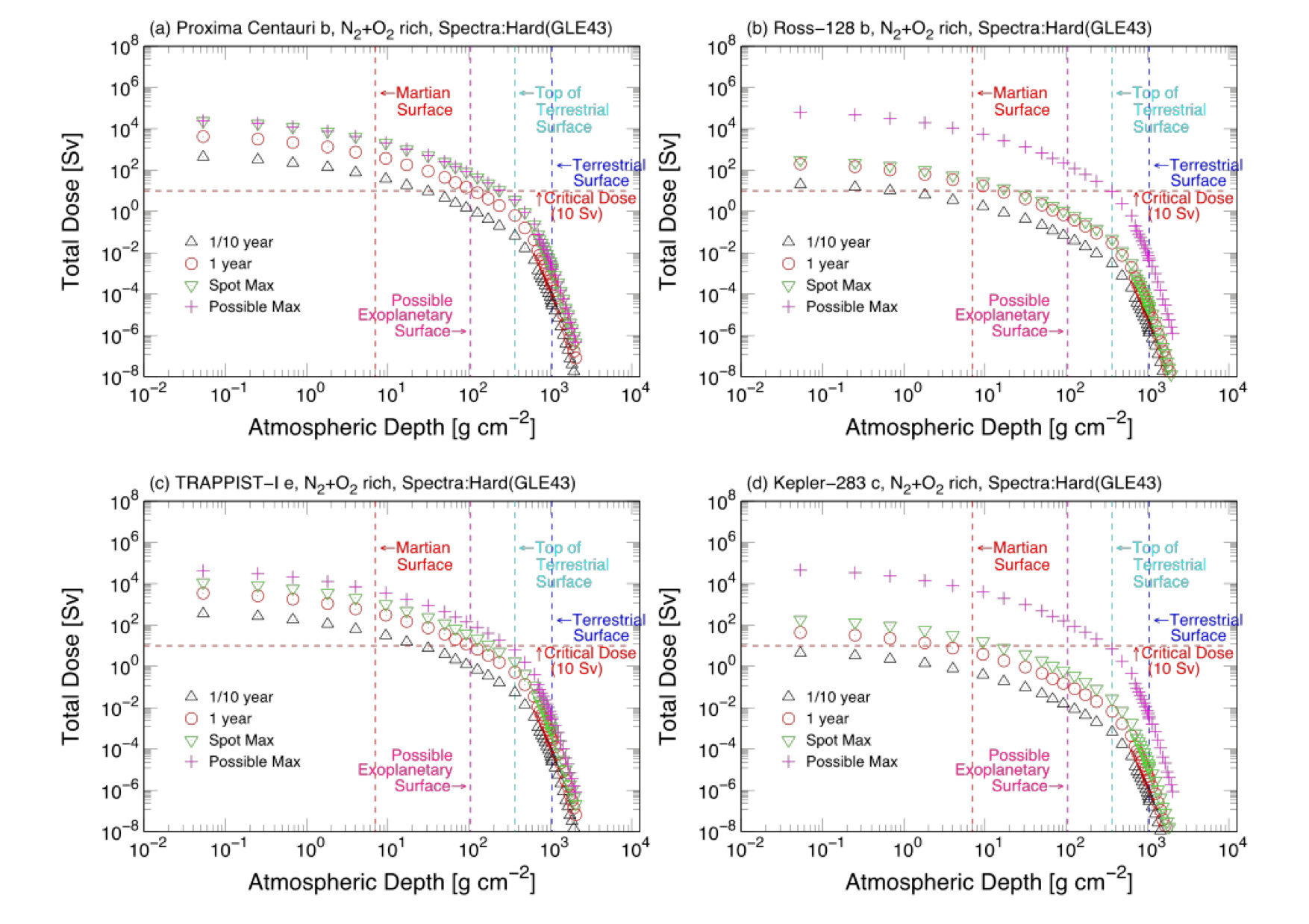 Figure 20
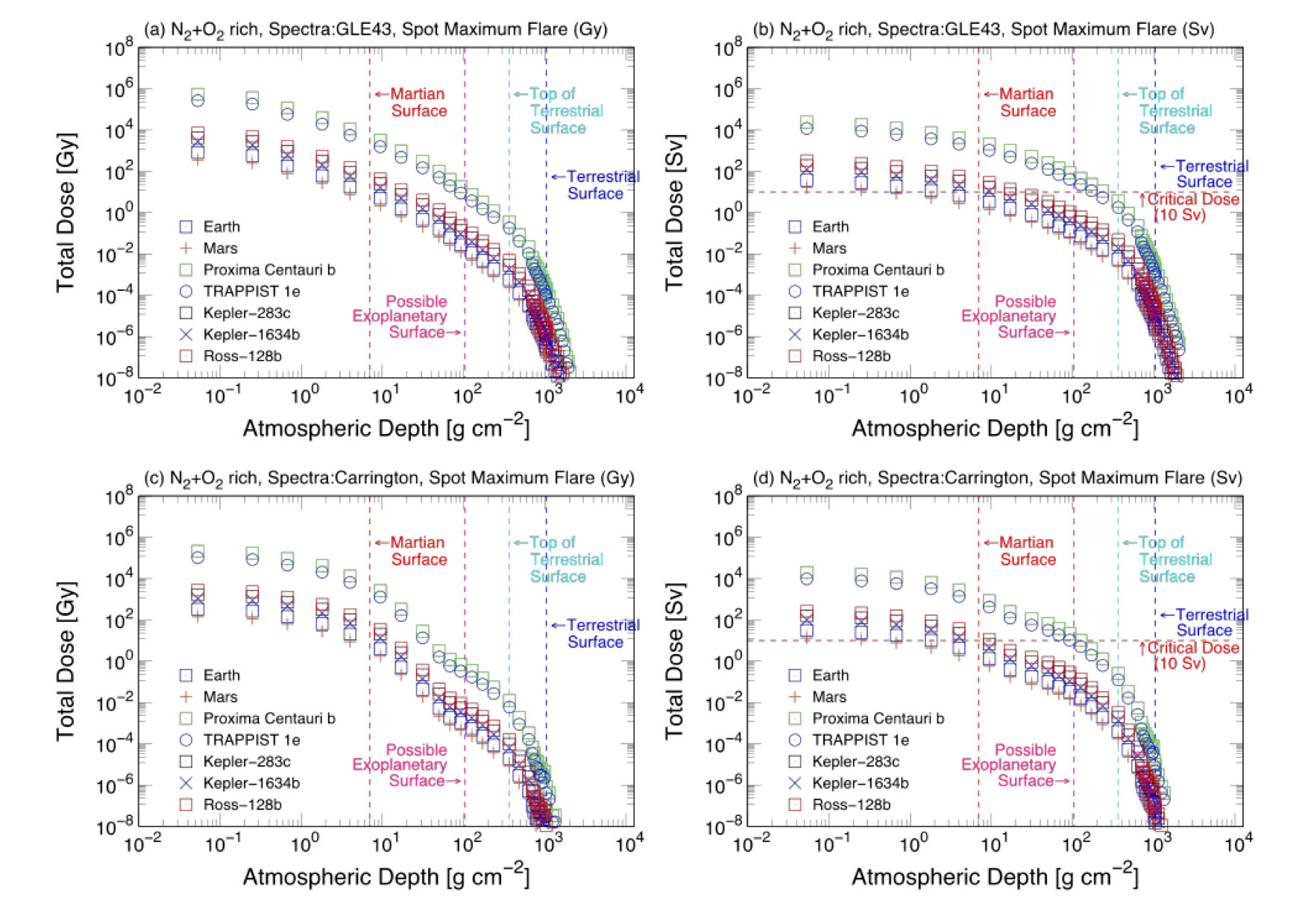 Figure 21
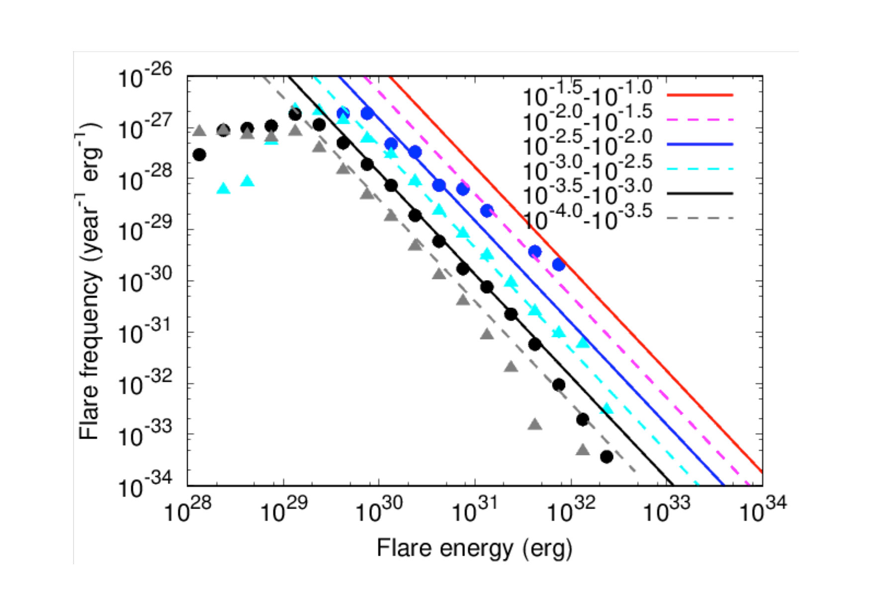 Figure 22
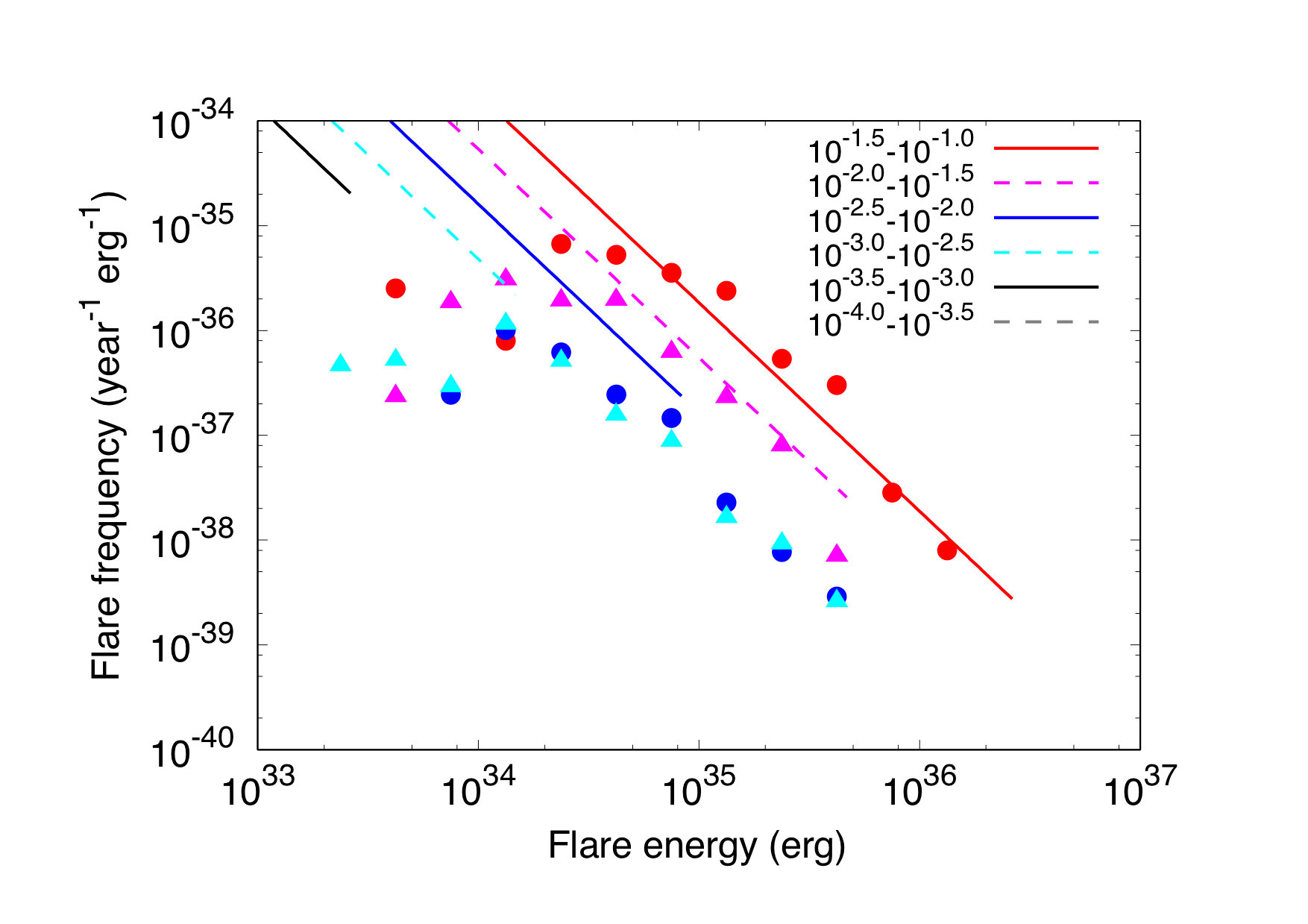 Figure 23
| Planet | Host star | |||||||||
|---|---|---|---|---|---|---|---|---|---|---|
| Exoplanet name | Radius | Size class | Mass | Spectra | Radius | Flare energy [erg] | ||||
| [] | [] | Type | [K] | [] | [day] | Annual | Spot Maximum | |||
| GJ 699 b | 1.37 | super-Earth-size | 3.23 | M4V | 3278 | 0.18 | 140.0 | 0.0003 | 6.26E+31 | 1.15E+32 |
| Kepler-283 c | 1.82 | super-Earth-size | 4.59 | K5 | 4141 | 0.64 | 18.2 | 0.0021 | 4.93E+32 | 2.13E+33 |
| Kepler-1634 b | 3.19 | Neptune-size | 7.77 | G7 | 5637 | 0.82 | 19.8 | 0.0066 | 1.65E+33 | 1.18E+34 |
| Proxima Cen b | 1.07 | Earth-size | 1.27 | M5.5V | 3050 | 0.14 | 82.6 | 0.0040 | 9.7E+32 | 5.55E+33 |
| Ross-128 b | 1.10 | Earth-size | 1.40 | M4 | 3192 | 0.20 | 121.0 | 0.0002 | 4.72E+31 | 7.72E+31 |
| TRAPPIST-1 b | 1.09 | Earth-size | 0.86 | M8 | 2550 | 0.12 | 3.3 | 0.0012 | 2.70E+32 | 9.09E+32 |
| TRAPPIST-1 c | 1.06 | Earth-size | 1.38 | M8 | 2550 | 0.12 | 3.3 | 0.0012 | 2.70E+32 | 9.09E+32 |
| TRAPPIST-1 d | 0.77 | Earth-size | 0.41 | M8 | 2550 | 0.12 | 3.3 | 0.0012 | 2.70E+32 | 9.09E+32 |
| TRAPPIST-1 e | 0.92 | Earth-size | 0.64 | M8 | 2550 | 0.12 | 3.3 | 0.0012 | 2.70E+32 | 9.09E+32 |
| TRAPPIST-1 f | 1.05 | Earth-size | 0.67 | M8 | 2550 | 0.12 | 3.3 | 0.0012 | 2.70E+32 | 9.09E+32 |
| TRAPPIST-1 g | 1.13 | Earth-size | 1.34 | M8 | 2550 | 0.12 | 3.3 | 0.0012 | 2.70E+32 | 9.09E+32 |
| TRAPPIST-1 h | 0.76 | Earth-size | 0.36 | M8 | 2550 | 0.12 | 3.3 | 0.0012 | 2.70E+32 | 9.09E+32 |
| Sol d (Earth) | 1.00 | Earth-size | 1.00 | G2V | 5778 | 1.00 | 25.0 | 0.0030 | 7.20E+32 | 3.64E+33 |
| Sol e (Mars) | 0.53 | Mars-size | 0.11 | G2V | 5778 | 1.00 | 25.0 | 0.0030 | 7.2E+32 | 3.64E+33 |
| Exoplanet | TOA | TOA | MS | MS | TM | TM | GL | GL | ||||||||
| Name | [Gy] | [Sv] | [Gy] | [Sv] | [Gy] | [Sv] | [Gy] | [Sv] | ||||||||
| [1] | [2] | [3] | [4] | [5] | [6] | [7] | [8] | |||||||||
| GJ 699 b | 8.72E+01 | 3.95E+00 | 5.20E-01 | 3.46E-01 | 5.82E-05 | 5.91E-04 | 2.31E-08 | 2.59E-07 | ||||||||
| Kepler-283 c | 9.64E+02 | 4.36E+01 | 5.75E+00 | 3.83E+00 | 6.44E-04 | 6.54E-03 | 2.56E-07 | 2.86E-06 | ||||||||
| Kepler-1634 b | 3.84E+02 | 1.74E+01 | 2.29E+00 | 1.53E+00 | 2.56E-04 | 2.61E-03 | 1.02E-07 | 1.14E-06 | ||||||||
| Proxima Centauri b | 9.37E+04 | 4.24E+03 | 5.60E+02 | 3.72E+02 | 6.26E-02 | 6.36E-01 | 2.49E-05 | 2.79E-04 | ||||||||
| Ross 128 b | 4.36E+03 | 1.97E+02 | 2.60E+01 | 1.73E+01 | 2.91E-03 | 2.96E-02 | 1.16E-06 | 1.30E-05 | ||||||||
| TRAPPIST-1 b | 4.97E+05 | 2.25E+04 | 2.97E+03 | 1.97E+03 | 3.32E-01 | 3.37E+00 | 1.32E-04 | 1.48E-03 | ||||||||
| TRAPPIST-1 c | 2.65E+05 | 1.20E+04 | 1.58E+03 | 1.05E+03 | 1.77E-01 | 1.80E+00 | 7.04E-05 | 7.88E-04 | ||||||||
| TRAPPIST-1 d | 1.33E+05 | 6.04E+03 | 7.97E+02 | 5.30E+02 | 8.91E-02 | 9.06E-01 | 3.54E-05 | 3.97E-04 | ||||||||
| TRAPPIST-1 e | 7.73E+04 | 3.50E+03 | 4.61E+02 | 3.07E+02 | 5.16E-02 | 5.25E-01 | 2.05E-05 | 2.30E-04 | ||||||||
| TRAPPIST-1 f | 4.46E+04 | 2.02E+03 | 2.66E+02 | 1.77E+02 | 2.98E-02 | 3.02E-01 | 1.18E-05 | 1.32E-04 | ||||||||
| TRAPPIST-1 g | 3.02E+04 | 1.37E+03 | 1.80E+02 | 1.20E+02 | 2.01E-02 | 2.05E-01 | 8.00E-06 | 8.96E-05 | ||||||||
| TRAPPIST-1 h | 1.55E+04 | 7.00E+02 | 9.22E+01 | 6.14E+01 | 1.03E-02 | 1.05E-01 | 4.10E-06 | 4.59E-05 | ||||||||
| Sol d (Earth) | 1.64E+02 | 7.40E+00 | 9.76E-01 | 6.50E-01 | 1.09E-04 | 1.11E-03 | 4.34E-08 | 4.86E-07 | ||||||||
| Sol e (Mars) | 7.05E+01 | 3.19E+00 | 4.21E-01 | 2.80E-01 | 4.71E-05 | 4.78E-04 | 1.87E-08 | 2.09E-07 | ||||||||
| [1] Estimated Dose [Gy] by Annual Maximum Flare at TOA | ||||||||||||||||
| [2] Estimated Dose [Sv] by Annual Maximum Flare at TOA | ||||||||||||||||
| [3] Estimated Dose [Gy] by Annual Maximum Flare at MS | ||||||||||||||||
| [4] Estimated Dose [Sv] by Annual Maximum Flare at MS | ||||||||||||||||
| [5] Estimated Dose [Gy] by Annual Maximum Flare at TM | ||||||||||||||||
| [6] Estimated Dose [Sv] by Annual Maximum Flare at TM | ||||||||||||||||
| [7] Estimated Dose [Gy] by Annual Maximum Flare at GL | ||||||||||||||||
| [8] Estimated Dose [Sv] by Annual Maximum Flare at GL | ||||||||||||||||
| TOA - Top of Atmosphere ( 0 g/cm2) | ||||||||||||||||
| MS - Martian Surface Atmospheric Pressure (9 g/cm2) | ||||||||||||||||
| TM - Terrestrial Minimum Atmospheric Pressure (365 g/cm2) | ||||||||||||||||
| GL - (Earth’s) Ground Level Atmospheric Pressure (1037 g/cm2) | ||||||||||||||||
| Exoplanet | TOA | TOA | MS | MS | TM | TM | GL | GL | ||||||||
| Name | [Gy] | [Sv] | [Gy] | [Sv] | [Gy] | [Sv] | [Gy] | [Sv] | ||||||||
| [9] | [10] | [11] | [12] | [13] | [14] | [15] | [16] | |||||||||
| GJ 699 b | 1.60E+02 | 7.25E+00 | 9.56E-01 | 6.37E-01 | 1.07E-04 | 1.09E-03 | 4.25E-08 | 4.76E-07 | ||||||||
| Kepler-283 c | 4.16E+03 | 1.89E+02 | 2.49E+01 | 1.65E+01 | 2.78E-03 | 2.83E-02 | 1.11E-06 | 1.24E-05 | ||||||||
| Kepler-1634 b | 2.74E+03 | 1.24E+02 | 1.64E+01 | 1.09E+01 | 1.83E-03 | 1.86E-02 | 7.27E-07 | 8.14E-06 | ||||||||
| Proxima Centauri b | 5.36E+05 | 2.43E+04 | 3.20E+03 | 2.13E+03 | 3.58E-01 | 3.64E+00 | 1.42E-04 | 1.59E-03 | ||||||||
| Ross 128 b | 7.13E+03 | 3.23E+02 | 4.26E+01 | 2.83E+01 | 4.77E-03 | 4.84E-02 | 1.89E-06 | 2.12E-05 | ||||||||
| TRAPPIST-1 b | 1.67E+06 | 7.58E+04 | 9.99E+03 | 6.65E+03 | 1.12E+00 | 1.14E+01 | 4.44E-04 | 4.97E-03 | ||||||||
| TRAPPIST-1 c | 8.93E+05 | 4.04E+04 | 5.33E+03 | 3.55E+03 | 5.96E-01 | 6.06E+00 | 2.37E-04 | 2.65E-03 | ||||||||
| TRAPPIST-1 d | 4.49E+05 | 2.03E+04 | 2.68E+03 | 1.79E+03 | 3.00E-01 | 3.05E+00 | 1.19E-04 | 1.34E-03 | ||||||||
| TRAPPIST-1 e | 2.60E+05 | 1.18E+04 | 1.55E+03 | 1.03E+03 | 1.74E-01 | 1.77E+00 | 6.91E-05 | 7.74E-04 | ||||||||
| TRAPPIST-1 f | 1.50E+05 | 6.79E+03 | 8.96E+02 | 5.96E+02 | 1.00E-01 | 1.02E+00 | 3.98E-05 | 4.46E-04 | ||||||||
| TRAPPIST-1 g | 1.02E+05 | 4.60E+03 | 6.06E+02 | 4.04E+02 | 6.78E-02 | 6.89E-01 | 2.69E-05 | 3.02E-04 | ||||||||
| TRAPPIST-1 h | 5.20E+04 | 2.36E+03 | 3.11E+02 | 2.07E+02 | 3.48E-02 | 3.53E-01 | 1.38E-05 | 1.55E-04 | ||||||||
| Sol d (Earth) | 8.27E+02 | 3.74E+01 | 4.93E+00 | 3.29E+00 | 5.52E-04 | 5.61E-03 | 2.19E-07 | 2.46E-06 | ||||||||
| Sol e (Mars) | 3.56E+02 | 1.61E+01 | 2.13E+00 | 1.42E+00 | 2.38E-04 | 2.42E-03 | 9.45E-08 | 1.06E-06 | ||||||||
| [1] Estimated Dose [Gy] by Annual Maximum Flare at TOA | ||||||||||||||||
| [2] Estimated Dose [Sv] by Annual Maximum Flare at TOA | ||||||||||||||||
| [3] Estimated Dose [Gy] by Annual Maximum Flare at MS | ||||||||||||||||
| [4] Estimated Dose [Sv] by Annual Maximum Flare at MS | ||||||||||||||||
| [5] Estimated Dose [Gy] by Annual Maximum Flare at TM | ||||||||||||||||
| [6] Estimated Dose [Sv] by Annual Maximum Flare at TM | ||||||||||||||||
| [7] Estimated Dose [Gy] by Annual Maximum Flare at GL | ||||||||||||||||
| [8] Estimated Dose [Sv] by Annual Maximum Flare at GL | ||||||||||||||||
| TOA - Top of Atmosphere ( 0 g/cm2) | ||||||||||||||||
| MS - Martian Surface Atmospheric Pressure (9 g/cm2) | ||||||||||||||||
| TM - Terrestrial Minimum Atmospheric Pressure (365 g/cm2) | ||||||||||||||||
| GL - (Earth’s) Ground Level Atmospheric Pressure (1037 g/cm2) | ||||||||||||||||
| Exoplanet | ||||||||||||||
| Name | [J m-2] | [%] | [J m-2] | [%] | [J m-2] | |||||||||
| [1] | [2] | [3] | [4] | [5] | [6] | [7] | ||||||||
| GJ 699 b | 8.74E+03 | 7.27E+04 | 2.59E06 | 4.37E+03 | 7.27E+04 | 2.51E02 | 2.35E+04 | |||||||
| Kepler-283 c | 4.43E+02 | 3.69E+03 | 1.31E07 | 2.22E+02 | 3.69E+03 | 1.27E03 | 1.19E+06 | |||||||
| Kepler-1634 b | 4.60E+04 | 3.83E+05 | 1.37E05 | 2.30E+04 | 3.83E+05 | 1.32E01 | 6.67E+05 | |||||||
| Proxima Cen b | 1.57E+04 | 1.31E+05 | 4.66E06 | 7.86E+03 | 1.31E+05 | 4.51E02 | 1.33E+07 | |||||||
| Ross-128 b | 8.75E+04 | 7.28E+05 | 2.60E05 | 4.38E+04 | 7.28E+05 | 2.51E01 | 1.38E+06 | |||||||
| TRAPPIST-1 b | 5.30E+04 | 4.41E+05 | 1.57E05 | 2.65E+04 | 4.41E+05 | 1.52E01 | 5.99E+07 | |||||||
| TRAPPIST-1 c | 2.82E+04 | 2.35E+05 | 8.39E06 | 1.41E+04 | 2.35E+05 | 8.11E02 | 3.20E+07 | |||||||
| TRAPPIST-1 d | 1.42E+04 | 1.18E+05 | 4.22E06 | 7.12E+03 | 1.18E+05 | 4.08E02 | 1.61E+07 | |||||||
| TRAPPIST-1 e | 8.24E+03 | 6.86E+04 | 2.45E06 | 4.12E+03 | 6.86E+04 | 2.37E02 | 9.32E+06 | |||||||
| TRAPPIST-1 f | 4.75E+03 | 3.96E+04 | 1.41E06 | 2.38E+03 | 3.96E+04 | 1.36E02 | 5.38E+06 | |||||||
| TRAPPIST-1 g | 3.22E+03 | 2.68E+04 | 9.54E07 | 1.61E+03 | 2.68E+04 | 9.23E03 | 3.64E+06 | |||||||
| TRAPPIST-1 h | 1.65E+03 | 1.37E+04 | 4.89E07 | 8.24E+02 | 1.37E+04 | 4.73E03 | 1.86E+06 | |||||||
| Sol d (Earth) | 3.70E01 | 3.08E+00 | 1.10E10 | 1.85E01 | 3.08E+00 | 1.06E06 | 1.74E+05 | |||||||
| Sol e (Mars) | 1.59E01 | 1.33E+00 | 4.72E11 | 7.96E02 | 1.33E+00 | 4.57E07 | 7.51E+04 | |||||||
| Exoplanet | ||||||||||||||
| Name | [J m-2] | [J m-2] | [J m-2] | [J m-2] | [J m-2] | |||||||||
| [8] | [9] | [10] | [11] | [12] | [13] | [14] | ||||||||
| GJ 699 b | 1.65E+06 | 8.68E+07 | 7.79E+08 | 2.79 E+04 | 0.16 | 1.66E+06 | 0.00 | |||||||
| Kepler-283 c | 4.25E+08 | 1.14E+10 | 2.83E+10 | 1.19E+06 | 6.82 | 4.25E+08 | 0.13 | |||||||
| Kepler-1634 b | 1.79E+09 | 1.14E+10 | 1.33E+10 | 6.90E+05 | 3.96 | 1.79E+0.9 | 0.53 | |||||||
| Proxima Cen b | 2.44E+07 | 8.78E+08 | 2.74E+10 | 1.33E+07 | 76.21 | 2.44E+07 | 0.01 | |||||||
| Ross-128 b | 9.25E+07 | 5.01E+09 | 5.81E+10 | 1.50E+06 | 8.61 | 9.25E+07 | 0.03 | |||||||
| TRAPPIST-1 b | 2.13E+08 | 8.97E+09 | 1.72E+11 | 7.29E+07 | 418.36 | 2.13E+08 | 0.06 | |||||||
| TRAPPIST-1 c | 1.14E+08 | 4.79E+09 | 9.19E+10 | 3.89E+07 | 223.21 | 1.14E+08 | 0.03 | |||||||
| TRAPPIST-1 d | 5.73E+07 | 2.41E+09 | 4.63E+10 | 1.96E+07 | 112.34 | 5.73E+07 | 0.02 | |||||||
| TRAPPIST-1 e | 3.32E+07 | 1.40E+09 | 2.68E+10 | 1.13E+07 | 65.07 | 3.32E+07 | 0.01 | |||||||
| TRAPPIST-1 f | 1.91E+07 | 8.05E+08 | 1.54E+10 | 6.54E+06 | 37.52 | 1.91E+07 | 0.01 | |||||||
| TRAPPIST-1 g | 1.30E+07 | 5.44E+08 | 1.05E+10 | 4.42E+06 | 25.39 | 1.30E+07 | 0.00 | |||||||
| TRAPPIST-1 h | 6.64E+06 | 2.79E+08 | 5.36E+09 | 2.27E+06 | 13.01 | 6.64E+06 | 0.00 | |||||||
| Sol d (Earth) | 3.37E+09 | 1.93E+10 | 2.04E+10 | 1.74E+05 | 1.00 | 3.37E+09 | 1.00 | |||||||
| Sol e (Mars) | 1.45E+09 | 8.32E+09 | 8.81E+09 | 7.51E+04 | 0.43 | 1.45E+09 | 0.43 | |||||||
| [1] UV Energy by Annual Maximum Flare at TOA | [2] Ratio to Earth’s Annual Maximum Flare | |||||||||||||
| [3] Ratio to Earth’s annual UV flux at TOA | [4] XUV Energy by Annual Maximum Flare at TOA | |||||||||||||
| [5] Ratio to Earth’s Annual Maximum Flare | [6] Ratio to Earth’s annual UV flux at TOA | |||||||||||||
| [7] Annual XUV Energy by Normal Stellar Radiation at TOA | ||||||||||||||
| [8] Annual UV Energy by Normal Stellar Radiation at TOA | ||||||||||||||
| [9] Annual Visible Ray Energy by Normal Stellar Radiation at TOA | ||||||||||||||
| [10] Annual IR Energy by Normal Stellar Radiation at TOA | ||||||||||||||
| [11] Annual Total (flare + Quiescent) XUV Energy at TOA | ||||||||||||||
| [12] Ratio to Earth / Annual Total (flare + Quiescent) XUV Energy at TOA | ||||||||||||||
| [13] Annual Total (flare + Quiescent) UV Energy at TOA | ||||||||||||||
| [14]Ratio to Earth / Annual Total (flare + Quiescent) UV Energy at TOA | ||||||||||||||
| TOA - Top of Atmosphere ( 0 g/cm2) | ||||||||||||||
| Exoplanet | ||||||||||||||
| Name | [J m-2] | [%] | [J m-2] | [%] | [J m-2] | |||||||||
| [1] | [2] | [3] | [4] | [5] | [6] | [7] | ||||||||
| Kepler-283 c | 8.24E+03 | 6.85E+04 | 2.44E06 | 4.12E+03 | 6.85E+04 | 2.36E02 | 1.01E+05 | |||||||
| Kepler-1634 b | 4.60E+04 | 3.83E+05 | 1.37E05 | 2.30E+04 | 3.83E+05 | 1.32E01 | 7.07E+05 | |||||||
| Proxima Cen b | 1.57E+04 | 1.31E+05 | 4.66E06 | 7.86E+04 | 1.31E+05 | 4.51E02 | 1.33E+07 | |||||||
| Ross-128 b | 8.75E+04 | 7.28E+05 | 2.60E05 | 4.38E+04 | 7.28E+05 | 2.51E01 | 1.38E+06 | |||||||
| TRAPPIST-1 b | 5.30E+04 | 4.41E+05 | 1.57E05 | 2.65E+04 | 4.41E+05 | 1.52E01 | 1.12E+08 | |||||||
| TRAPPIST-1 c | 2.83E+04 | 2.35E+05 | 8.39E06 | 1.41E+04 | 2.35E+05 | 8.11E02 | 5.99E+07 | |||||||
| TRAPPIST-1 d | 1.42E+04 | 1.18E+05 | 4.22E06 | 7.12E+03 | 1.18E+05 | 4.08E02 | 3.01E+07 | |||||||
| TRAPPIST-1 e | 8.24E+03 | 6.86E+04 | 2.45E06 | 4.12E+03 | 6.86E+04 | 2.37E02 | 1.75E+07 | |||||||
| TRAPPIST-1 f | 4.75E+03 | 3.96E+04 | 1.41E06 | 2.38E+03 | 3.96E+04 | 1.36E02 | 1.01E+07 | |||||||
| TRAPPIST-1 g | 3.22E+03 | 2.68E+04 | 9.54E07 | 1.61E+03 | 2.68E+04 | 9.23E03 | 6.81E+06 | |||||||
| TRAPPIST-1 h | 1.65E+03 | 1.37E+04 | 4.89E07 | 8.24E+02 | 1.37E+04 | 4.73E03 | 3.49E+06 | |||||||
| Sol d (Earth) | 3.70E01 | 3.08E+00 | 1.10E10 | 1.85E01 | 3.08E+00 | 1.06E06 | 1.74E+05 | |||||||
| Sol e (Mars) | 1.60E01 | 1.33E+00 | 4.72E11 | 7.96E02 | 1.33E+00 | 4.57E07 | 7.51E+04 | |||||||
| Exoplanet | ||||||||||||||
| Name | [J m-2] | [J m-2] | [J m-2] | [J m-2] | [J m-2] | |||||||||
| [8] | [9] | [10] | [11] | [12] | [13] | [14] | ||||||||
| Kepler-283 c | 1.96E+09 | 1.12E+10 | 1.19E+10 | 1.05E+05 | 0.60 | 1.96E+09 | 0.58 | |||||||
| Kepler-1634 b | 1.90E+09 | 1.21E+10 | 1.41E+10 | 7.30E+03 | 4.19 | 1.90E+0.9 | 0.56 | |||||||
| Proxima Cen b | 2.44E+07 | 8.78E+08 | 2.74E+10 | 1.33E+07 | 76.21 | 2.44E+07 | 0.01 | |||||||
| Ross-128 b | 9.24E+07 | 5.01E+09 | 5.81E+10 | 1.42E+06 | 8.17 | 9.25E+07 | 0.03 | |||||||
| TRAPPIST-1 b | 2.53E+08 | 8.97E+09 | 1.72E+11 | 1.12E+08 | 644.10 | 2.53E+08 | 0.07 | |||||||
| TRAPPIST-1 c | 1.35E+08 | 4.79E+09 | 9.19E+10 | 5.99E+07 | 343.66 | 1.35E+08 | 0.04 | |||||||
| TRAPPIST-1 d | 6.79E+07 | 2.41E+09 | 4.63E+10 | 3.01E+07 | 172.95 | 6.79E+07 | 0.02 | |||||||
| TRAPPIST-1 e | 3.93E+07 | 1.40E+09 | 2.68E+10 | 1.75E+07 | 100.19 | 3.97E+07 | 0.01 | |||||||
| TRAPPIST-1 f | 2.27E+07 | 8.04E+08 | 1.54E+10 | 1.01E+07 | 57.76 | 2.27E+07 | 0.01 | |||||||
| TRAPPIST-1 g | 1.53E+07 | 5.44E+08 | 1.05E+10 | 6.81E+06 | 39.09 | 1.53E+07 | 0.00 | |||||||
| TRAPPIST-1 h | 7.86E+06 | 2.79E+08 | 5.36E+09 | 3.49E+06 | 20.03 | 7.86E+06 | 0.00 | |||||||
| Sol d (Earth) | 3.37E+09 | 1.93E+10 | 2.04E+10 | 1.74E+05 | 1.00 | 3.37E+09 | 1.00 | |||||||
| Sol e (Mars) | 1.45E+09 | 8.32E+09 | 8.81E+09 | 750E+04 | 0.43 | 1.45E+09 | 0.43 | |||||||
| [1] UV Energy by Annual Maximum Flare at TOA | [2] Ratio to Earth’s Annual Maximum Flare | |||||||||||||
| [3] Ratio to Earth’s annual UV flux at TOA | [4] XUV Energy by Annual Maximum Flare at TOA | |||||||||||||
| [5] Ratio to Earth’s Annual Maximum Flare | [6] Ratio to Earth’s annual UV flux at TOA | |||||||||||||
| [7] Annual XUV Energy by Normal Stellar Radiation at TOA | ||||||||||||||
| [8] Annual UV Energy by Normal Stellar Radiation at TOA | ||||||||||||||
| [9] Annual Visible Ray Energy by Normal Stellar Radiation at TOA | ||||||||||||||
| [10] Annual IR Energy by Normal Stellar Radiation at TOA | ||||||||||||||
| [11] Annual Total (flare + Quiescent) XUV Energy at TOA | ||||||||||||||
| [12] Ratio to Earth / Annual Total (flare + Quiescent) XUV Energy at TOA | ||||||||||||||
| [13] Annual Total (flare + Quiescent) UV Energy at TOA | ||||||||||||||
| [14] Ratio to Earth of Annual Total (flare + Quiescent)UV Energy at TOA | ||||||||||||||
| TOA - Top of Atmosphere ( 0 g/cm2) | ||||||||||||||
Peer Reviews
No public reviews on file for this paper yet. If you reviewed it on a platform where reviews are public (OpenReview, ICLR, NeurIPS, ICML), you can paste yours below so the community can read it here.
Videos
No videos yet. Explain this paper in a talk, walkthrough, or lecture? Add one.
Taxonomy
TopicsStellar, planetary, and galactic studies · Gamma-ray bursts and supernovae · Astro and Planetary Science
Impact of Stellar Superflares on Planetary Habitability
Yosuke A. Yamashiki
Graduate School of Advanced Integrated Studies in Human Survivability, Kyoto University, Sakyo, Kyoto, Japan
Unit of the Synergetic Studies for Space, Kyoto University, Sakyo, Kyoto, Japan
Okayama Branch Office, Subaru Telescope, National Astronomical Observatory of Japan, NINS, Kamogata, Asakuchi, Okayama, Japan
Okayama Observatory, Kyoto University, Kamogata, Asakuchi, Okayama, Japan
NASA/GSFC/SEEC, Greenbelt, MD, USA
American University, DC, USA
Laboratory for Atmospheric and Space Physics, University of Colorado Boulder, Boulder, CO, USA
National Solar Observatory, Boulder, CO, USA
Department of Astronomy, Kyoto University, Sakyo, Kyoto, Japan
Tatsuhiko Sato
Nuclear Science and Engineering Center Center, Japan Atomic Energy Agency (JAEA), Tokai, Ibaraki, Japan
Leiden Observatory, Leiden University, Leiden, The Netherlands
Department of Astronomy, Kyoto University, Sakyo, Kyoto, Japan
Ryusuke Kuroki
Graduate School of Advanced Integrated Studies in Human Survivability, Kyoto University, Sakyo, Kyoto, Japan
Keiya Murashima
Faculty of Science, Kyoto University, Sakyo, Kyoto, Japan
Hiroaki Sato
Faculty of Engineering, Kyoto University, Sakyo, Kyoto, Japan
Department of Astronomy, Kyoto University, Sakyo, Kyoto, Japan
Department of Astronomy, Kyoto University, Sakyo, Kyoto, Japan
Unit of the Synergetic Studies for Space, Kyoto University, Sakyo, Kyoto, Japan
Thomas B. Scott
Interface Analysis Centre, University of Bristol, Bristol, UK
Hina Bando
Faculty of Science, Kyoto University, Sakyo, Kyoto, Japan
Subaru Nashimoto
Faculty of Science, Kyoto University, Sakyo, Kyoto, Japan
Fuka Takagi
Faculty of Agriculture, Kyoto University, Sakyo, Kyoto, Japan
Cassandra Ling
Graduate School of Advanced Integrated Studies in Human Survivability, Kyoto University, Sakyo, Kyoto, Japan
Daisaku Nogami
Department of Astronomy, Kyoto University, Sakyo, Kyoto, Japan
Unit of the Synergetic Studies for Space, Kyoto University, Sakyo, Kyoto, Japan
Kazunari Shibata
Astronomical Observatory, Kyoto University, Sakyo, Kyoto, Japan
Unit of the Synergetic Studies for Space, Kyoto University, Sakyo, Kyoto, Japan
(Received 17 April 2019; Revised 26 May 2019; Accepted 16 June 2019)
Abstract
High-energy radiation caused by exoplanetary space weather events from planet-hosting stars can play a crucial role in conditions promoting or destroying habitability in addition to the conventional factors. In this paper, we present the first quantitative impact evaluation system of stellar flares on the habitability factors with an emphasis on the impact of Stellar Proton Events. We derive the maximum flare energy from stellar starspot sizes and examine the impacts of flare associated ionizing radiation on CO2, H2, N2+O2 –rich atmospheres of a number of well-characterized terrestrial type exoplanets. Our simulations based on the Particle and Heavy Ion Transport code System [PHITS] suggest that the estimated ground level dose for each planet in the case of terrestrial-level atmospheric pressure (1 bar) for each exoplanet does not exceed the critical dose for complex (multi-cellular) life to persist, even for the planetary surface of Proxima Centauri b, Ross-128 b and TRAPPIST-1 e. However, when we take into account the effects of the possible maximum flares from those host stars, the estimated dose reaches fatal levels at the terrestrial lowest atmospheric depth on TRAPPIST-1 e and Ross-128 b. Large fluxes of coronal XUV radiation from active stars induces high atmospheric escape rates from close-in exoplanets suggesting that the atmospheric depth can be substantially smaller than that on the Earth. In a scenario with the atmospheric thickness of 1/10 of Earth’s, the radiation dose from close-in planets including Proxima Centauri b and TRAPPIST-1 e reach near fatal dose levels with annual frequency of flare occurrence from their hoststars.
††journal: ApJ
1 Introduction
The definition of habitable zones for extrasolar planetary systems is traditionally based on the conditions promoting the presence of standing bodies of liquid surface water (determined as CHZ: Conventional Habitable Zone), but other more refined boundaries may be considered (Kopparapu et al., 2013; Ramirez et al., 2019). For example, the inner habitable boundary may be defined by critical fluxes, which cause runaway/moisture greenhouse effects (Kasting, 1988) while the outer boundary may be constrained by the presence of carbon dioxide in the atmosphere as gas phase, avoiding its condensation (Kasting et al., 1993). The exoplanets within CHZs around active stars can be subject to high ionizing radiation fluxes including X-ray and Extreme Ultraviolet Emission (referred as to XUV (1-1200 ) Emission),coronal mass ejections (CMEs) and associated stellar energetic particles (SEP) events that can affect exoplanetary habitability conditions (Airapetian et al. 2017a; Airapetian et al. 2019).
Energetic stellar flare events associated with coronal mass ejections (CME) from magnetically active stars can contribute to the generation of stellar transient XUV emission and form high-energy particles accelerated in CME driven shocks (Kumari et al. 2017; Gopalswamy et al. 2017; Airapetian et al. 2019). These SEPs can penetrate into exoplanetary atmospheres, and cause chemical changes. These changes can be positive for the initiation of prebiotic chemistry in the planetary atmospheres or detrimental due to the destruction of a large fraction of ozone that transmits UVC (1000-2800 ) and UVB (2800-3150 ) emission to the exoplanetary surfaces (Airapetian et al. 2016; Airapetian et al. 2017b; Segura et al. 2010; Tilley et al. 2019).
Our own Sun is known to exhibit extreme flare activity in the past including the so-called Carrington-class event (Townsend et al., 2006). Recent observations by the Kepler space telescope revealed that young solar-type stars generate much higher frequency of energetic flares (superflares), which could have been an important factor for habitability in the early history of our solar system and/or most extrasolar systems (Maehara et al., 2012; Shibayama et al., 2013; Takahashi et al., 2016; Notsu et al., 2019; Airapetian et al., 2019). Extreme surges of were detected in the tree rings (Miyake et al. 2012; Miyake et al. 2013), which is considered strong evidence of the occurrence of superflares more than one magnitude stronger than the Carrington-class event (Usoskin et al., 2013). Effects of stellar activity from their host stars may also include periodic sterilizing doses of radiation via stellar superflare activity (Lingam & Loeb, 2017). While the frequency and maximum energy of solar and stellar flares from planet hosts have not been well characterized, they may present a critical limiting factor on the development and persistence of life on terrestrial-type planets in our solar system (Jakosky et al. 2015; Schrijver et al. 2015;Kay et al. 2016) as well as on Earth-sized exoplanets (Atri, 2017). Thus, a consistent approach to determine the habitable zone accounting for these factors is required. The characterization of these factors can be made using recently derived correlation between stellar flare frequency/intensity and starspot area, found from Kepler data, which may overcome the difficulty in prediction of flare impacted system (Maehara et al., 2017).
Here, we present the first comprehensive impact evaluation system of expected ground level radiation doses in close-in terrestrial type exoplanets around M dwarfs including Proxima Centauri b (see Table 1) in response to severe Solar Proton Events (SPEs). This study represents a realistic model of the surface dose evaluation for exoplanets with various possible atmospheric pressures and compositions. Section 1 presents the framework for evaluation of SPE particle fluence at the top of exoplanetary atmospheres. In Section 2 we discuss the application of the Particle and Heavy Ion Transport code System (PHITS) to a number of close-in exoplanets around M dwarfs. Section 3 discusses the ground dose for various exoplanetary systems and their consequences for the biological habitability of complex lifeforms. Section 4 describes the conclusions of the paper and future work.
2 Method
2.1 Outline of Fluence Estimation for Top of Atmosphere (TOA) on Each Planet from Stellar Proton Events, and Definition of Maximum Flare Energy
Our analysis is based on the application of stellar flare and starspot data derived mostly from the Kepler mission (Maehara et al. 2015; Maehara et al. 2017; Notsu et al. 2013; Notsu et al. 2015a; Notsu et al. 2015b; Notsu et al. 2019), in the ExoKyoto exoplanetary database (Yamashiki et al. 2019, in preparation). Our method utilizes starspot data derived from optical light curves to be used in parametric studies of the thickness of hypothetical exoplanetary atmospheres as the major attenuation factor of the incident radiation[see Table 1]. These data are used as input for the Particle and Heavy Ion Transport code System - PHITS (Sato et al., 2018a) Monte-Carlo simulation model that is used for simulations of surface dose for terrestrial type exoplanets.
The following equations derive an assumed stellar flare magnitude from observed stellar spot size data. For the estimation of spot size, we used the same method in Maehara et al. 2017. Figures 1 and 2 illustrate flare frequency vs flare energy for solar flares. The solid line and dotted line represent the estimated scaling low calculated using equation (1) as a different starspot area derived from Maehara et al. (2017).
Using the results of the above study, we derived the flare frequency distribution over its energy in the optical band as a function of the stellar spot size as follows:
[TABLE]
in which : Flare frequency (year -1), : Total area of starspots, : Total visible area of the stellar surface, : Total expected stellar flare energy (erg), and : Flare frequency constant (1029.4).
Here we define and set as 1, we then may determine Annual Maximum Flare energy as follows:
[TABLE]
in which : Annual Maximum Flare energy, as total expected stellar flare energy per year (erg year*-1* ), , .
The Spot Maximum Flare, maximum flare energy under a determined starspot area, can be illustrated as
[TABLE]
in which : Fraction of magnetic energy that can be released as flare energy, : Magnetic-field strength, : Spot Maximum Flare energy, as the theoretical maximum flare energy with a determined starspot area (erg), and : Solar radius ( cm ).
Possible Maximum Flare energy in this study was determined through the following (1) Evaluate maximum starspot coverage of the star through observation of stellar lightcurves. In this study, we observed a 20% coverage of starspot on Proxima Centauri; accordingly we determined the maximum starspot coverage as 20%. Then, (3) calculate maximum energy induced by the starspot area by Shibata et al. (2013).
The outline of the estimation method is as follows:
(STEP 1) Derive the magnitude and frequency of Stellar Proton Events from each star (1) by using direct observation of a stellar flare as a proxy of an SPE energy; and (2) by applying the starspot area and/or rotational period correlation methodology. The conversion equation is presented and discussed in the next section. We use above information to extract representative starspot areas which can be applied to the conversion equations to flare energy expressed in the following section. Accordingly we obtain (a) Annual Maximum flare (see equation(2)) Spot Maximum flare (see equation(3)) (Aschwanden et al. 2017; Shibata et al. 2013), and (c) Possible Maximum Flare, calculated assuming that the target star surface is covered with starspots under the maximum percentage of observed starspot area (set as 20% of half the spherical area).
(STEP 2) After the above procedure is completed for each star system, the possible quantitative exposures are assumed by the following procedure: (4) Estimating the fluence of each Stellar Proton Event at the TOA using the equation (A4) .
As for the atmospheric compositions of exoplanets, three-types of atmospheres for typical extrasolar planets are considered (explained in detail in the following section). For those typical atmospheric compositions, the potential doses for life on extrasolar planets are determined through the following procedure.
(STEP 3) (5) Calculate the possible dose rate from the Monte-Carlo simulations using Particle and Heavy Ion Transport code System PHITS (Sato et al., 2018a) for three typical atmospheric compositions as extrasolar planetary atmospheres, (6) Normalize the dose by determining the Earth equivalent ratio, which was previously normalized by using (6a) The Carrington-class event, assuming that the event has X45 class, or by (6b) The deepest observed flare event GLE43 which occurred in 1989, as X13 class (Xapsos et al. , 2000). (7) Calculate conversion coefficients for each exoplanet by comparing the values calculated in (4) and (6). (8) Convert the reference dose value calculated in (6) into each extrasolar planet case using conversion coefficients.
2.2 Monte Carlo Simulation for Air-Shower using PHITS
When high-energy SEPs precipitate into the planetary atmosphere, they induce extensive air-shower (EAS) by producing various secondary particles, such as neutrons and muons. We conducted a three-dimensional EAS simulation by using the Particle and Heavy Ion Transport code System, PHITS (Sato et al., 2018a), which is a general-purpose Monte Carlo code for analyzing the propagation of radiation in any materials. PHITS version 2.88 with the recommended setting for cosmic-ray transport simulation (Sato et al., 2014) was used in this survey. In our simulations we assume the size and the mass of the modeled planets to be the same as that of the Earth.
2.3 Chemical Composition of Exoplanetary Atmospheres
The impact of stellar proton events on a planet depends upon its atmospheric composition. We consider three: Earth-like (N2+O2 rich), Mars-like or Venus-like (CO2 rich) and an young Earth-sized or super-Earth’s with a primary H2 rich atmospheres. We assume that the Earth-type atmosphere is the standard land-ocean planetary atmosphere composed mostly of Nitrogen and Oxygen (N2+O2). A Venusian-like atmosphere is represented as a CO2 -rich atmosphere resulted from the runaway greenhouse effect and subsequent outgassing of CO2 from carbonates. The Martian-like atmosphere is an example of a low gravity low pressure planetary CO2 -rich atmosphere that has experienced severe atmospheric escape driven by strong stellar ionizing radiation flux. We also model a young Earth-sized H2 rich atmosphere, because such an atmosphere is assumed for large super-Earth planets, whose gravitational pull might be sufficiently large to retain substantial atmospheric H2. Hydrogen rich atmospheres of Earth-sized exoplanets can be formed due to capture of hydrogen from protoplanetary atmospheres and/or during accretion period (Elkins-Tanton and Seafer 2008; Lammer et al. 2018). Thus, here we refer to young Earth-sized exoplanets.
The composition of the atmosphere, for the above three typical atmospheric types, were set to 78% nitrogen, 21% oxygen and 1% argon for the Earth-like (N2+O2) atmosphere, for the Martian/Venusian-type (CO2), and 100% hydrogen for the young-Earth-type (H2). During the Monte-Carlo simulation using PHITS, we assume the composition of the planet interior to be covered with sufficient liquid water for the Terrestrial-type, while the same gas was continuously filled in the planet interior for the other cases. In our simulation of all model atmosphere (young Earth-type(H2), Earth-like (N2+O2), Martian and Venusian-type (CO2)) cases we assume the exoplanet radius and mass to be 1 REarth and 1 MEarth, respectively. Numerical simulation of super-Earths will be performed in the upcoming studies.
2.4 Event Integrated Spectra of Extreme SPEs
We assume that stellar accelerated protons are isotropically distributed in space as they precipitate into the atmospheres of the modeled planets and have two different energy spectra represented by the SPE spectra derived for the Carrington-class event in 1859 (Townsend et al., 2006) and the 43rd ground level enhancement (GLE) in 1989 (Xapsos et al. , 2000), respectively.
The Carrington-class event is considered to be the largest eruptive event recorded in modern human history. However, according to Smart et al. (2006), proton energy spectra associated with the Carrington-class event was rather soft in comparison with other solar flares that produce GLEs. Thus, the radiation dose at the ground level during the event is expected to be not significantly high, because only a small fraction of the high-energy protons (with energies over 3 GeV for an 1-bar atmosphere) and their secondary particles can penetrate into the deep atmosphere.
To estimate the maximum impact on the ground level, we therefore calculated the radiation dose during the solar flare in association with a harder proton spectrum, GLE43, which is one of the most significant GLE that has occurred after satellite observations were started in the late 20th century. It should be noted that GLE 43 was selected as a typical SPE associated with a hard proton spectrum to estimate the maximum impact of SPE exposure at deeper locations in the atmosphere, though its flare class was not extremely high (X13). GLE 5 (23 Feb 1956) type spectra were also considered as a relevant event for the survey.
Figure 3 illustrates event-integrated spectra of the GLE43 that occurred on 19 October 1989 (solid) and the Carrington Flare that occurred on 1 September 1859 (dotted) solar proton events, based on parameters obtained from references.
2.5 The Influence of the Planetary Magnetic Field
We have simulated four scenarios of exoplanetary dipole magnetic moments: (i) B = 0 (unmagnetized planet), (ii) , (iii) (Earth-likle magnetic moment), and (iv) . The impact of the planetary magnetic field on the surface dose was modeled via the magnetospheric filter functions for the above 4 different magnetic moments, 0, 0.1, 1, and 10 , evaluated by Grießmeier et al. (2015).
The fluence of protons, neutrons, positive and negative muons, electrons, positrons, and photons were scored as a function of the atmospheric depth. They were then converted to the absorbed dose in Gy and the effective dose in Sv, using the stopping power and the fluence to the dose conversion coefficients for the isotropic irradiation (ICRP, 2010), respectively. It should be mentioned that the effective dose is defined as only used for the purpose of radiological protection. However we evaluated it for discussing the possible exposure effects on human-like lifeforms because there is no alternative quantity that can be used for this discussion. More detailed descriptions on the simulation procedures as well as their verification results for the solar energetic particle and galactic cosmic-ray simulation in the terrestrial atmosphere were given in our previous papers (Sato et al. 2015; Sato et al. 2018b).
The impacts of all components produced by cosmic-ray interactions with the different atmospheric types in different layers were also individually evaluated and finally integrated to produce a final ground level dose value for each simulated scenario. By examining all these different parameters together (atmospheric composition, geomagnetic field strength and simulated cosmic ray interactions), we have evaluated the atmospheric barrier needed for life on each of the target planets to survive a stellar flare event. This approach assumes that the potential life is as similarly radiation tolerant as that present on Earth.
2.6 The Maximum Stellar Flare Energy
Our goal is to study the effect of high ionizing particle fluxes caused by stellar activity on habitability of close-in Earth-sized and super Earth exoplanets located within habitable zones. CHZs around low luminosity M dwarfs are located within 0.05 AU that suggests that many of them orbit their host stars within sub Alfvenic distance and are subject to direct irradiation via high particle fluxes. To study the resulted surface dose we selected four exoplanets around active M dwarfs, one exoplanet around K dwarfs with detected superflare, and one exoplanet around G dwarf with higher stellar activity than our sun. We selected the target stars for this survey according to the following procedure (1) Select host star with exoplanet in habitable zone with direct superflare observation through Kepler observation (Kepler-283) (2) Select Kepler stars whose flare frequency and magnitude can be estimated from their activities (Kepler-1634) and (3) Select well-documented host star for well-documented exoplanets (GJ699 (Barnards Star), Proxima Centauri, Ross-128, TRAPPIST-I). Stellar activities for all stars are estimated using their light curves.
Shibata et al. (2013) estimated the maximum value (upper limit) of flare energy, which is determined by the starspot area and magnetic field strength. We used this methodology to calculate the theoretical maximum flare energy for six host stars using their starspot areas: erg for GJ 699 (Barnard’s Star), erg for Kepler-283, erg for Kepler-1634, erg for Proxima Centauri, erg for Ross 128, and erg for TRAPPIST-1.
In this method, the current observed starspot area in each star restricts the maximum flare energy. However, it is unclear whether the observed period represents the maximum or minimum activity of the star. Accordingly, we also evaluated the potential maximum energy of the stellar flare by the following method.
For those stars whose stellar temperature is above 4000 K: we estimated maximum flare energy based on the relationship between Kepler stars by comparing their maximum observed energy and stellar temperature as well as its associated radius (H. Maehara, private communication).
For those stars whose stellar temperature is below 4000 K: we assumed, in the extreme situation, that 20 % of the stellar surface is covered by starspot. Considering the extreme condition, we calculated the maximum energy using Shibata et al. (2013).
By introducing flare energy as input for considerable maximum energy of the superflares for their planetary systems, we may theoretically calculate the possible maximum dose for their host planets.
3 Results
3.1 Validation for Normal Dose
Figure 4 shows the vertical profile of radiation dose on Earth and Mars caused by SPEs with the hard proton spectrum (imitating GLE 43) (a)(b) and soft spectrum (imitating Carrington) (c)(d) penetrating N2+O2 rich (terrestrial-type) atmosphere Earth with erg (black triangle), erg (red circle), erg (blue square) and erg (red cross) in Gray (Gy) (a) (c) and Sievert (Sv) (b) (d). This figure shows that the radiation dose at the tropopose (around 170 g/cm2 atmospheric depth) becomes 0.5 Millisievert which agrees mostly with the aerial observation, when the solar flare energy is scaled to . Note that this normalization has been made for an idealized series of flares, considering the horizontal angle of the SPE injection as 90 degrees, in other words, the probability of reaching Earth is 1/4.
Figures 5 and 6 show vertical profile of radiation dose in Gray (5) and in Sievert(6) on Earth and Mars for possible flares on several different scales, caused by hard proton spectrum (imitating GLE 43) (a)(c) and soft spectrum (imitating Carrington reproduced by (Townsend et al., 2006)) (b)(d) penetrating N2+O2 rich (terrestrial-type) atmosphere for Earth (a)(b) and CO2 rich (Martian type) atmosphere for Mars(c)(d) with flares every 1/10 year (36 days, corresponding 7.2 erg), one year (corresponding 7.2 erg), Spot Maximum flare (corresponding 3.6 ergs) and Possible Maximum flare (corresponding 1.6 erg). In these scenarios, the Spot Maximum flare is the maximum possible flare to be observed within decades in the target stellar system (in this case our solar system) estimated based on starspot area of the target star. According to the calculation shown in these figures, the Solar Proton Events under the above scenarios do not induce a critical dose at ground level when we have sufficient atmospheric depth such as Earth, even under Possible Maximum flare (1.6 erg) scenario, whereas it becomes a nearly critical dose on the Martian surface with thinner atmospheric depth when the Spot Maximum flare (3.6 ergs) event occurs.
3.2 Estimated Dose on Exoplanetary Surface Under Different Flare Scenarios
The estimated doses under the Annual Maximum flare and under the Spot Maximum flare are shown in Tables 3.2 and 3.2, respectively. The estimated doses at the Top of Atmosphere (TOA) on GJ 699 b, Proxima Cen b, Ross-128 b and TRAPPIST-1 e under the Spot Maximum Flare (Shibata et al., 2013) becomes 1.60 Gy (7.25 Sv), 5.36 Gy (2.43 Sv) , 7.13 Gy (3.23 Sv), and 2.60 Gy (1.18 Sv), respectively.
The reference list from the paper itself. Each links out to its DOI / PubMed record.
- 1Airapetian et al. (2016) Airapetian, V. S., Glocer, A., Gronoff, G., Hébrard, E., & Danchi, W. 2016, Nature Geoscience, 9, 452
- 2Airapetian et al. (2017 a) Airapetian, V. S., Glocer, A., Khazanov, G. V., et al. 2017 a, Ap J, 836, L 3
- 3Airapetian et al. (2017 b) Airapetian, V. S., Jackman, C., Mlynzcak, M., Danchi, W.,& Hunt, M. , 2017 b, Scientific Reports, 7, 14141
- 4Airapetian et al. (2019) Airapetian, V. et al. 2019, International Journal of Astrobiology, eprint ar Xiv:1905.05093
- 5Aschwanden et al. (2017) Aschwanden, M. J., Caspi, A., Cohen, C. M. S., et al. 2017, Ap J, 836, 17
- 6Atri (2017) Atri, D. 2017, MNRAS, 465, L 34
- 7Cohen et al. (2014) Cohen, O., Drake, J. J., Glocer, A., et al. 2014, Ap J, 790, 57
- 8Davenport (2016) Davenport, J. R. A. 2016, Ap J, 829, 23