Excitation of Kerr quasinormal modes in extreme--mass-ratio inspirals
Jonathan Thornburg, Barry Wardell, Maarten van de Meent

TL;DR
This paper investigates the excitation of Kerr quasinormal modes during extreme-mass-ratio inspirals, revealing that these wiggles are a common, observable phenomenon that depends on black hole spin and orbital parameters, with implications for testing general relativity.
Contribution
It provides a comprehensive survey of QNM excitation phenomena in EMRIs, highlighting their observability and dependence on system parameters, and discusses their potential for testing gravity.
Findings
Wiggles are a generic feature across a wide parameter space.
QNM excitations are most prominent with high black hole spin and eccentric prograde orbits.
Wiggles could enable direct observation of Kerr QNMs in gravitational wave signals.
Abstract
If a small compact object orbits a black hole, it is known that it can excite the black hole's quasinormal modes (QNMs), leading to high-frequency oscillations ("wiggles") in the radiated field at , and in the radiation-reaction self-force acting on the object after its orbit passes through periapsis. Here we survey the phenomenology of these wiggles across a range of black hole spins and equatorial orbits. In both the scalar-field and gravitational cases we find that wiggles are a generic feature across a wide range of parameter space, and that they are observable in field perturbations at fixed spatial positions, in the self-force, and in radiated fields at . For a given charge or mass of the small body, the QNM excitations have the highest amplitudes for systems with a highly spinning central black hole, a prograde orbit with high eccentricity, and an…
Click any figure to enlarge with its caption.
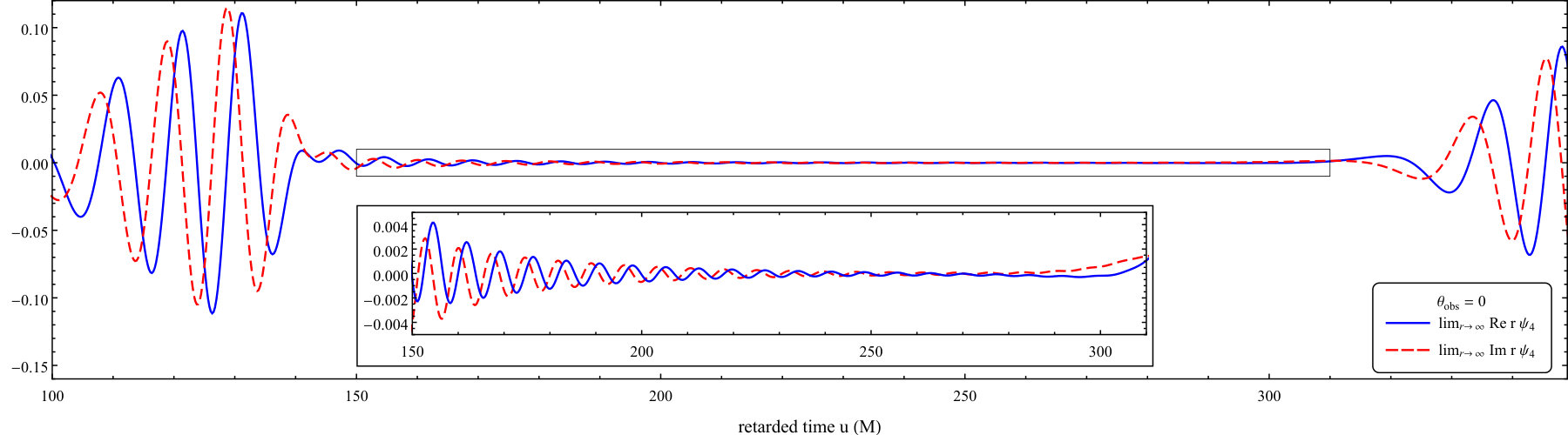 Figure 1
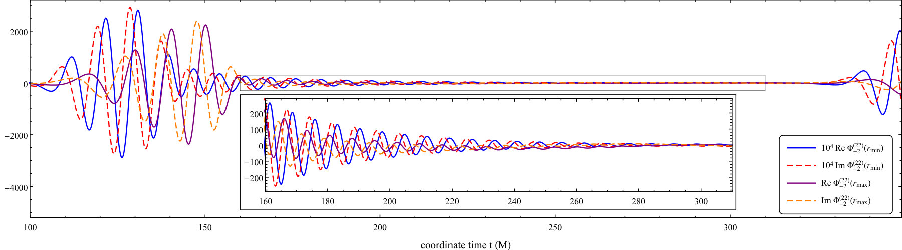 Figure 2
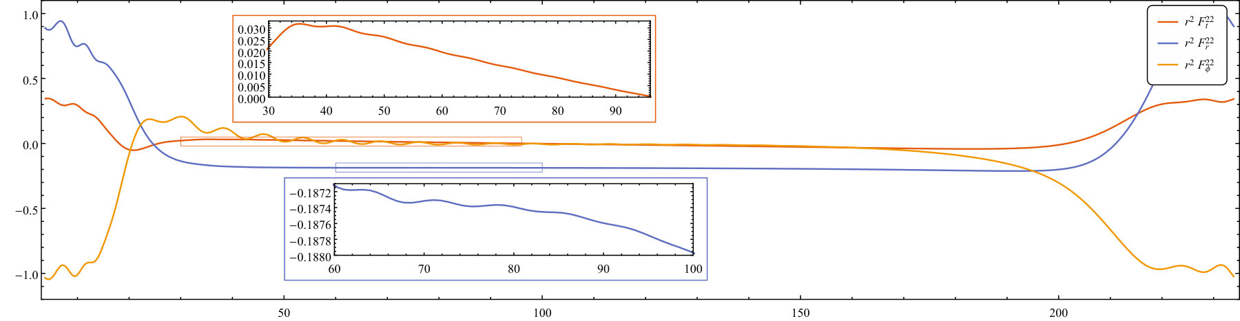 Figure 3
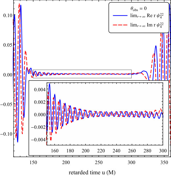 Figure 4
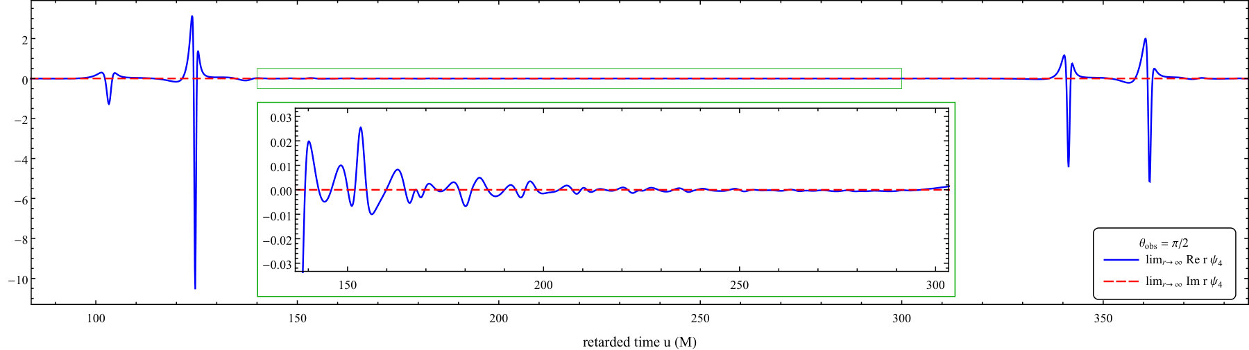 Figure 5
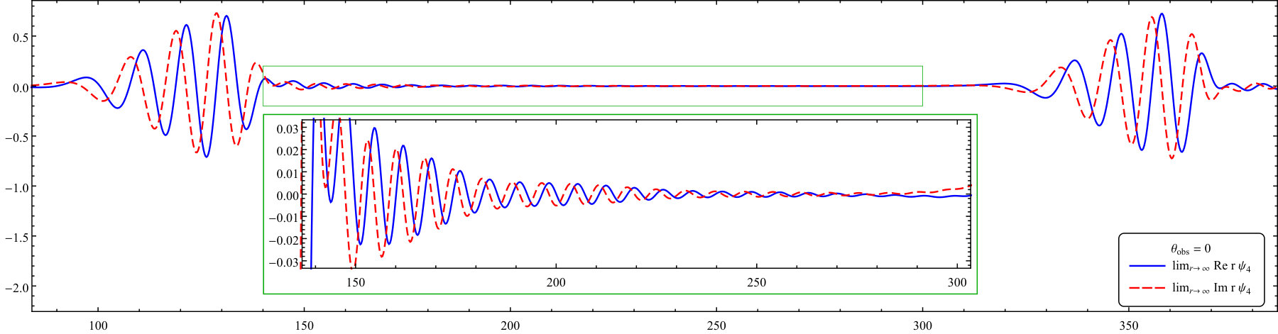 Figure 6
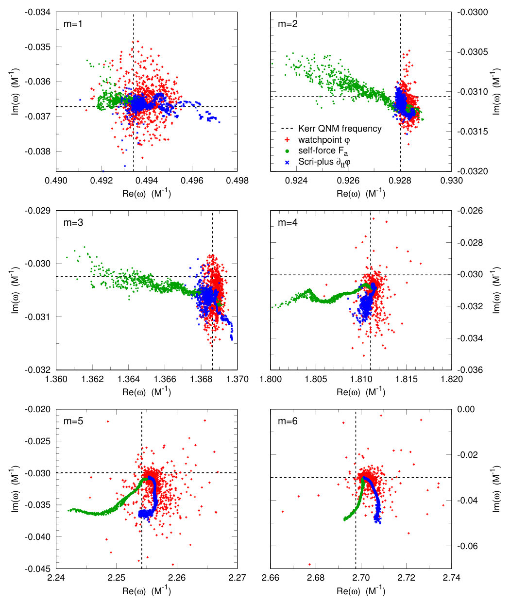 Figure 7
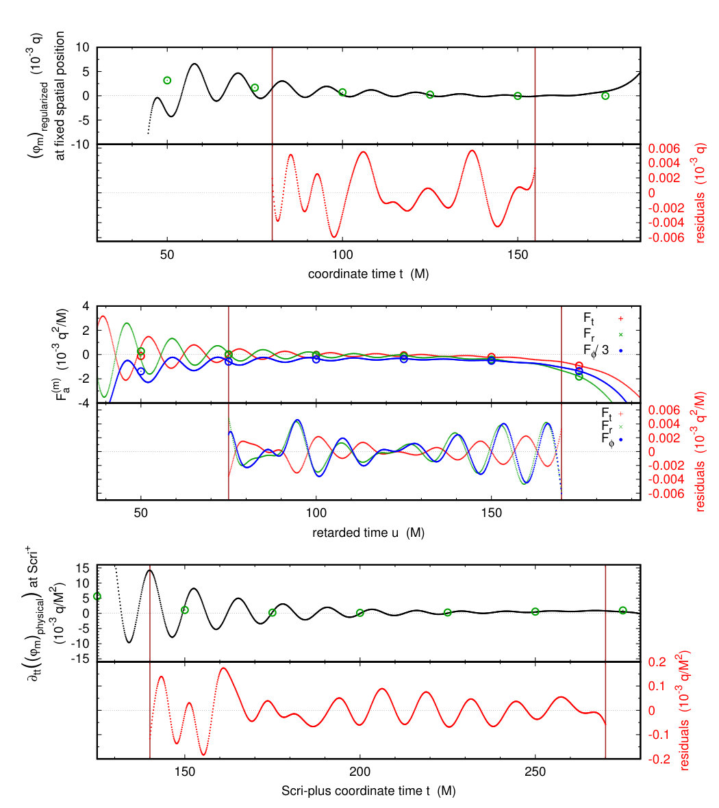 Figure 8
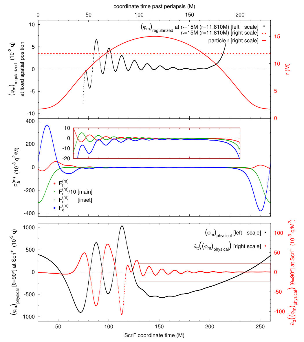 Figure 9
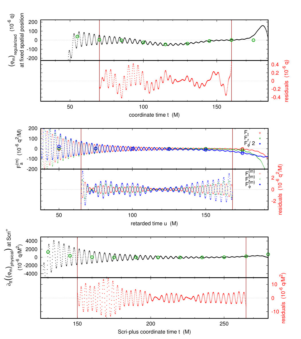 Figure 10
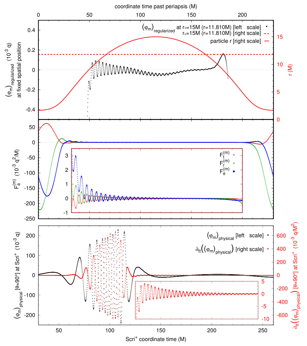 Figure 11
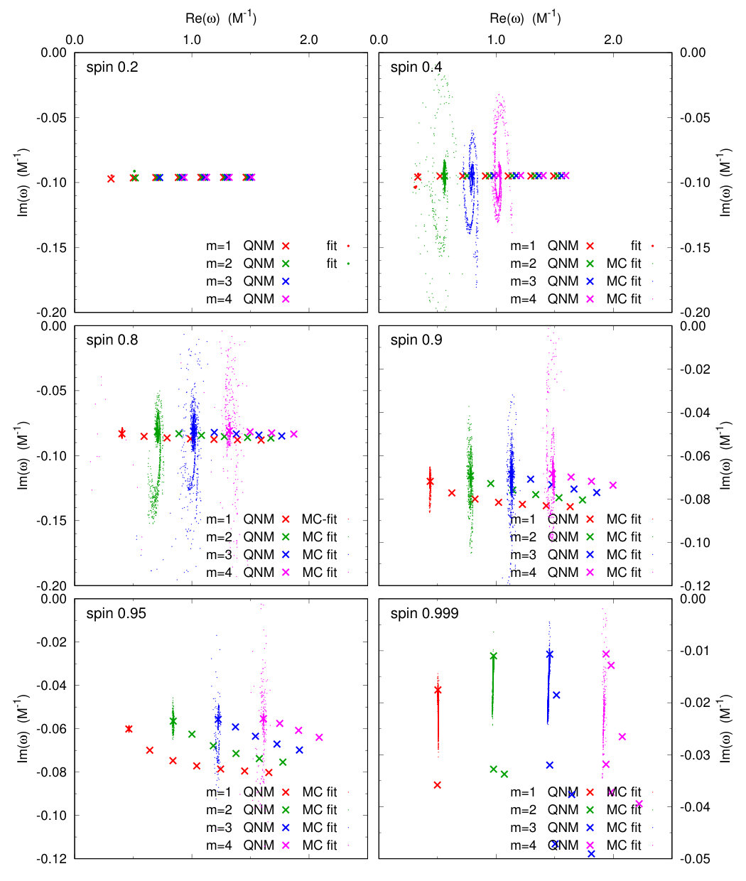 Figure 12
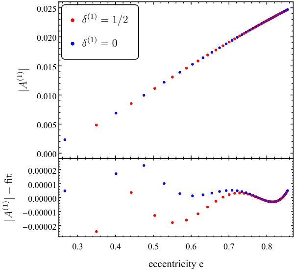 Figure 13
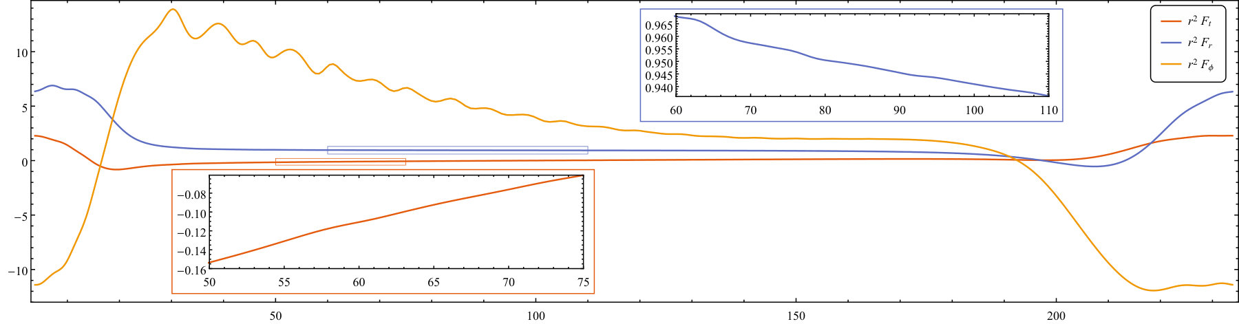 Figure 14
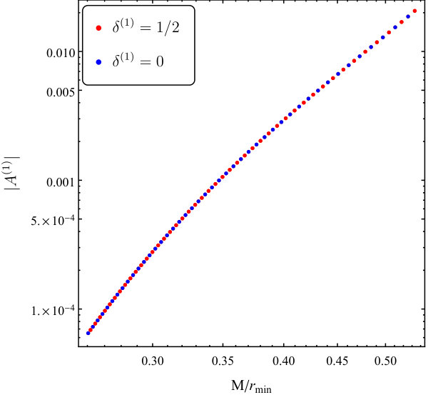 Figure 15
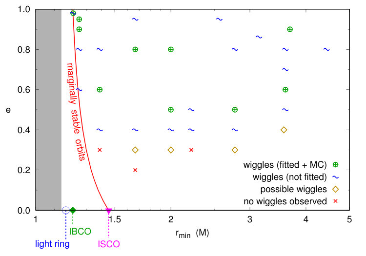 Figure 16
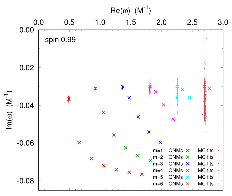 Figure 17
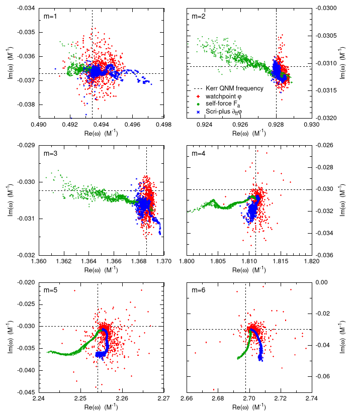 Figure 18
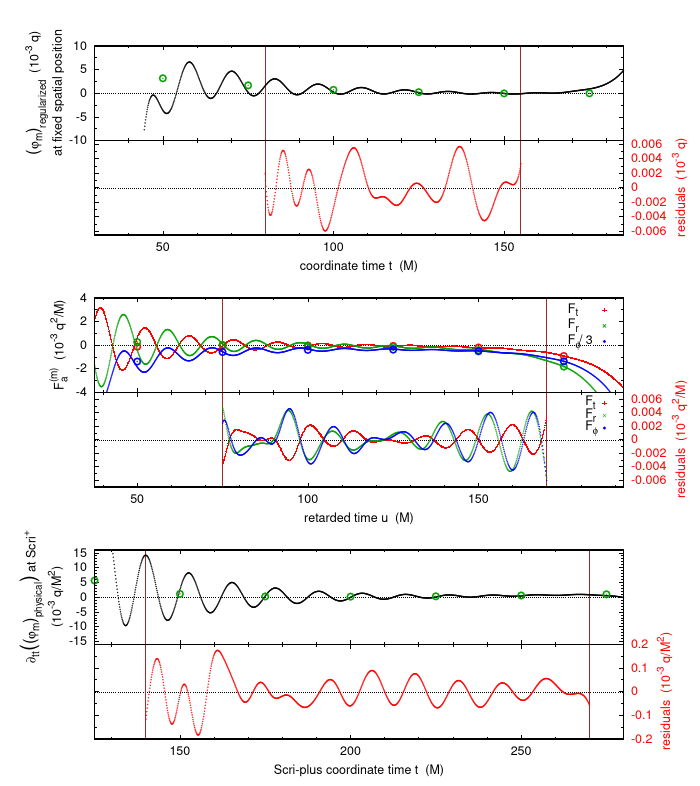 Figure 19
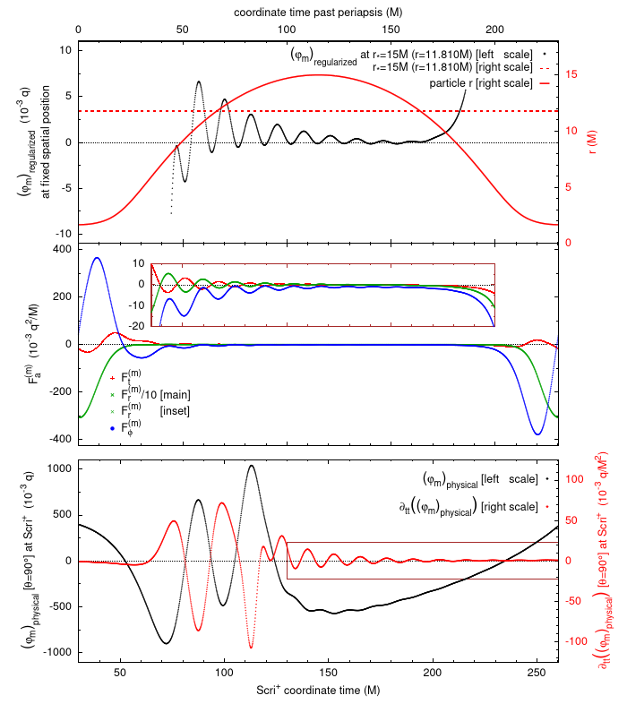 Figure 20
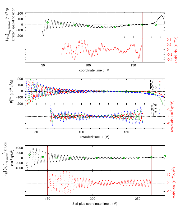 Figure 21
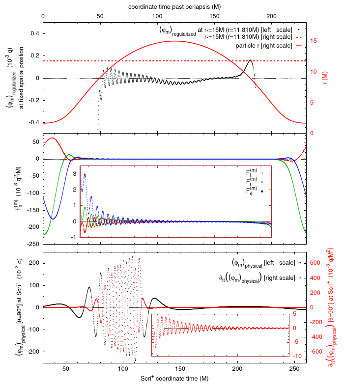 Figure 22
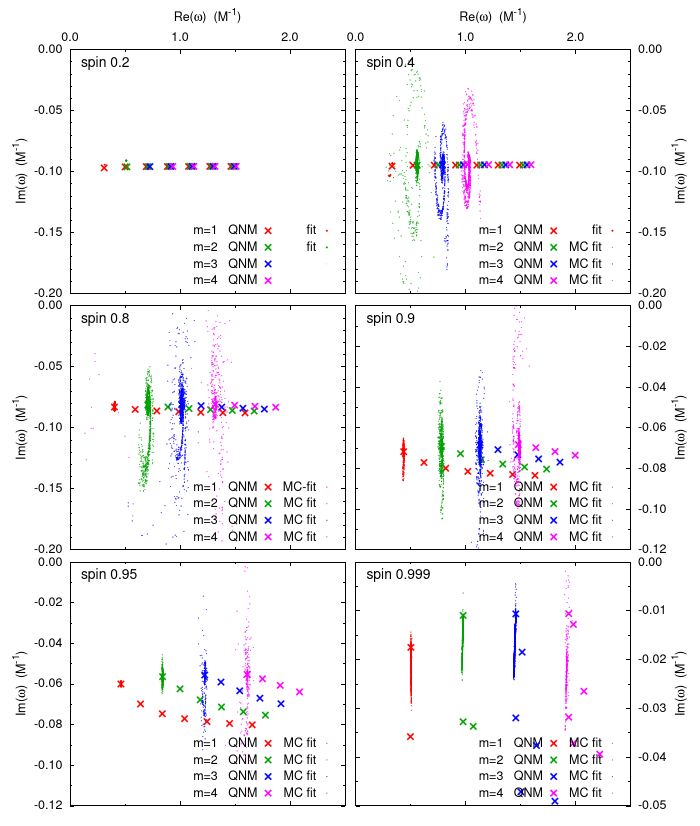 Figure 23
 Figure 24
| Field perturbation at … | Scalar field | Gravitational |
|---|---|---|
| fixed spatial position | ||
| (strong-field) | ||
| particle position | ||
| Name | Resolution | m=1 | m=2 | m=3 | m=4 | m=5 | m=6 | |||||||||||||||||||
| () | () | () | () | w | w | w | w | w | w | |||||||||||||||||
| w9x5-161 | 0.344 414 | dro12-96 | ||||||||||||||||||||||||
| w9x4-368 | 0.145 444 | dro8-64 | ||||||||||||||||||||||||
| w999-278 | 0.199 135 | dro10-80 | ||||||||||||||||||||||||
| w999-368 | 0.145 443 | dro8-64 | ||||||||||||||||||||||||
| ze98a | 0.430 498 | dro6-48 | ||||||||||||||||||||||||
| ze98 | 0.430 300 | dro10-80 | ||||||||||||||||||||||||
| w99-125a | 0.421 924 | dro8-64 | ||||||||||||||||||||||||
| w99-125b | 0.421 555 | dro8-64 | ||||||||||||||||||||||||
| w99-125c | 0.420 811 | dro6-48 | ||||||||||||||||||||||||
| w99-125d | 0.419 300 | dro8-64 | ||||||||||||||||||||||||
| w99-139 | 0.389 231 | dro8-64 | ||||||||||||||||||||||||
| w99-139b | 0.386 760 | dro8-64 | ||||||||||||||||||||||||
| w99-139d | 0.384 220 | dro6-48 | ||||||||||||||||||||||||
| w99-139c | 0.382 960 | dro6-48 | ||||||||||||||||||||||||
| w99-167m | 0.336 304 | dro8-64 | ||||||||||||||||||||||||
| w99-167 | 0.333 682 | dro10-80 | ||||||||||||||||||||||||
| w99-167k | 0.326 143 | dro6-48 | ||||||||||||||||||||||||
| w99-167d | 0.324 141 | dro6-48 | ||||||||||||||||||||||||
| w99-167j | 0.322 115 | dro6-48 | ||||||||||||||||||||||||
| w99-200d | 0.281 145 | dro8-64 | ||||||||||||||||||||||||
| w99-200 | 0.274 441 | dro6-48 | ||||||||||||||||||||||||
| w99-200b | 0.272 062 | dro6-48 | ||||||||||||||||||||||||
| w99-200c | 0.269 607 | dro6-48 | ||||||||||||||||||||||||
| w99-222b | 0.245 832 | dro6-48 | ||||||||||||||||||||||||
| w99-222 | 0.243 319 | dro6-48 | ||||||||||||||||||||||||
| w99-222c | 0.240 719 | dro6-48 | ||||||||||||||||||||||||
| e95 | 0.220 775 | dro8-64 | ||||||||||||||||||||||||
| w99-278 | 0.199 076 | dro8-64 | ||||||||||||||||||||||||
| w99-278b | 0.191 854 | dro8-64 | ||||||||||||||||||||||||
| w99-278c | 0.189 278 | dro6-48 | ||||||||||||||||||||||||
| w99-278d | 0.186 607 | dro6-48 | ||||||||||||||||||||||||
| s99 | 0.174 409 | dro6-48 | ||||||||||||||||||||||||
| w99-357 | 0.139 748 | dro6-48 | ||||||||||||||||||||||||
| w99-360c | 0.147 411 | dro6-48 | ||||||||||||||||||||||||
| w99-360b | 0.145 260 | dro6-48 | ||||||||||||||||||||||||
| w99-360a | 0.143 040 | dro8-64 | ||||||||||||||||||||||||
| w99-360j | 0.140 745 | dro6-48 | ||||||||||||||||||||||||
| e9 | 0.145 429 | dro8-64 | ||||||||||||||||||||||||
| w99-444 | 0.113 763 | dro6-48 | ||||||||||||||||||||||||
| w95-368 | 0.145 349 | dro6-48 | ||||||||||||||||||||||||
| n96 | 0.151 199 | dro8-64 | ||||||||||||||||||||||||
| w9-368 | 0.145 202 | dro6-48 | ||||||||||||||||||||||||
| n95 | 0.062 994 | dro8-64 | ||||||||||||||||||||||||
| w8-368 | 0.144 751 | dro6-48 | ||||||||||||||||||||||||
| e8b | 0.113 578 | dro6-48 | ||||||||||||||||||||||||
| e8 | 0.113 000 | dro8-64 | ||||||||||||||||||||||||
| w4-368 | 0.140 816 | dro6-48 | ||||||||||||||||||||||||
| w2-368 | 0.137 622 | dro6-48 | ||||||||||||||||||||||||
| ze4 | 0.106 691 | dro6-48 | ||||||||||||||||||||||||
| zze9 | 0.120 223 | dro8-64 | ||||||||||||||||||||||||
| ze9 | 0.120 222 | dro6-48 | ||||||||||||||||||||||||
| ns5 | 0.095 855 | dro8-64 | ||||||||||||||||||||||||
| s0 | 0.070 830 | dro4-32 | ||||||||||||||||||||||||
| n-55 | 0.062 012 | dro6-48 | ||||||||||||||||||||||||
| s-6 | 0.048 498 | dro4-32 | ||||||||||||||||||||||||
| wm8-631 | 0.066 625 | dro4-32 | ||||||||||||||||||||||||
| wm99-605 | 0.072 312 | dro4-32 | ||||||||||||||||||||||||
| s-99 | 0.038 531 | dro4-32 | ||||||||||||||||||||||||
| Symbol | Meaning |
|---|---|
| we observed oscillations in the diagnostics, successfully fit the appropriate wiggle model described in section IV.1 over a or range of wiggle periods, and performed the Monte-Carlo error analysis described in section IV.1.5. | |
| we observed oscillations in the diagnostics and successfully fit the appropriate wiggle model described in section IV.1, but the model was fitted over too short a or range ( wiggle periods) for the Monte-Carlo error analysis described in section IV.1.5 to be used | |
| we observed oscillations in the diagnostics which visually appeared to be wiggles, with physically reasonable period and decay rate, but we did not attempt to quantitatively fit a wiggle model | |
| we observed oscillations in the diagnostics which might have been wiggles, but these oscillations were not clearly separated from the background variation in the diagnostics | |
| we did not observe wiggle-like oscillations in the diagnostics; this could mean either that no wiggles are present, or alternatively that wiggles were present but they were at too low an amplitude and/or insufficiently separated from the background variation to be observed | |
| (blank) | diagnostics were not computed, not computed sufficiently accurately for studying wiggles, or were computed but not assessed |
| coarsest grid | finest grid | |||
| () | (radians) | () | (radians) | |
| dro12-96 | ||||
| dro10-80 | ||||
| dro8-64 | ||||
| dro6-48 | ||||
| dro4-32 | ||||
| 2 | 0 |
|
|
||||
|---|---|---|---|---|---|---|---|
| 2 | 1 |
|
|
||||
| 3 | 1 |
|
|
||||
| 2 | 2 |
|
|
||||
| 3 | 2 |
|
|
||||
| 4 | 2 |
|
|
||||
| 3 | 3 |
|
|
||||
| 4 | 3 |
|
|
||||
| 5 | 3 |
|
|
||||
| 4 | 4 |
|
|
||||
| 5 | 4 |
|
|
||||
| 5 | 5 |
|
|
Peer Reviews
No public reviews on file for this paper yet. If you reviewed it on a platform where reviews are public (OpenReview, ICLR, NeurIPS, ICML), you can paste yours below so the community can read it here.
Videos
No videos yet. Explain this paper in a talk, walkthrough, or lecture? Add one.
Excitation of Kerr quasinormal modes in extreme–mass-ratio inspirals
Jonathan Thornburg
Department of Astronomy and Center for Spacetime Symmetries, Indiana University, Bloomington, Indiana 47405, USA
Max-Planck-Institut für Gravitationsphysik, Albert-Einstein-Institut, Am Mühlenberg 1, D-14476 Potsdam-Golm, Germany
Barry Wardell
School of Mathematics and Statistics, University College Dublin, Belfield, Dublin 4, DO4 V1W8, Ireland
Maarten van de Meent
Max-Planck-Institut für Gravitationsphysik, Albert-Einstein-Institut, Am Mühlenberg 1, D-14476 Potsdam-Golm, Germany
Mathematical Sciences and STAG Research Centre, University of Southampton, Southampton, SO17 1BJ, United Kingdom
Abstract
If a small compact object orbits a black hole, it is known that it can excite the black hole’s quasinormal modes (QNMs), leading to high-frequency oscillations (“wiggles”) in the radiated field at , and in the radiation-reaction self-force acting on the object after its orbit passes through periapsis. Here we survey the phenomenology of these wiggles across a range of black hole spins and equatorial orbits. In both the scalar-field and gravitational cases we find that wiggles are a generic feature across a wide range of parameter space, and that they are observable in field perturbations at fixed spatial positions, in the self-force, and in radiated fields at . For a given charge or mass of the small body, the QNM excitations have the highest amplitudes for systems with a highly spinning central black hole, a prograde orbit with high eccentricity, and an orbital periapsis close to the light ring. The QNM amplitudes depend smoothly on the orbital parameters, with only very small amplitude changes when the orbit’s (discrete) frequency spectrum is tuned to match QNM frequencies. The association of wiggles with QNM excitations suggest that they represent a situation where the nonlocal nature of the self-force is particularly apparent, with the wiggles arising as a result of QNM excitation by the compact object near periapsis, and then encountered later in the orbit. Astrophysically, the effects of wiggles at might allow direct observation of Kerr QNMs in extreme-mass-ratio inspiral (EMRI) binary black hole systems, potentially enabling new tests of general relativity.
I Introduction
Consider a small (compact) body of mass (with ) moving freely near a Schwarzschild or Kerr black hole of mass . This system emits gravitational radiation, and there is a corresponding radiation-reaction influence on the small body’s motion. Calculating the resulting perturbed spacetime (including the small body’s motion and the emitted gravitational radiation) is a long-standing research question in general relativity.
There is also an astrophysical motivation for this calculation: If a neutron star or stellar-mass black hole of mass – orbits a massive black hole of mass –,111 denotes the solar mass. the resulting “extreme–mass-ratio inspiral” (EMRI) system is expected to be a strong astrophysical gravitational-wave (GW) source detectable by the planned Laser Interferometer Space Antenna (LISA) space-based gravitational-wave detector. LISA is expected to observe many such systems, some of them at quite high signal-to-noise ratios (Gair et al. (2004); Barack and Cutler (2004); Amaro-Seoane et al. (2007); Gair (2009)). The data analysis for, and indeed the detection of, such systems will generally require matched-filtering the detector data stream against appropriate precomputed GW templates. The problem of computing such templates provides an astrophysical motivation for EMRI modelling.
In the test-particle limit it has long been known that an unbound (scattering) flyby can excite quasinormal modes (QNMs) of the background black hole. Kojima and Nakamura Kojima and Nakamura (1984) studied this process, finding that “A scattered particle excites the quasi-normal mode under the condition that twice the angular velocity at the periapsis is greater than the real part of the frequency of the quasi-normal mode”. Their figure 3(b) shows an example of the QNM oscillations in the radiated gravitational waves at .
Burko and Khanna Burko and Khanna (2007) found small oscillations in the total radiated energy flux from a test particle making a parabolic (unbound) flyby of a Kerr black hole. They attributed these oscillations to the particle encountering scattered gravitational waves emitted during the particle’s inbound motion.
O’Sullivan and Hughes O’Sullivan and Hughes (2016) observed “small-amplitude high-frequency oscillations” in their calculations of the horizon shear of a Kerr black hole orbited by a test particle. Because they did not find corresponding oscillations in the horizon’s tidal distortion field, and their measured oscillation frequencies did not match known Kerr QNM frequencies, they concluded that the horizon-shear oscillations they observed “cannot be related to the [Kerr black] hole’s quasi-normal modes”.
Thornburg and Wardell Thornburg and Wardell (2017) (hereinafter TW) calculated the scalar-field self-force for eccentric equatorial particle orbits in Kerr spacetime. For some systems where the Kerr black hole was highly spinning and the particle orbit was prograde and highly eccentric, TW found that the self-force exhibits large oscillations (“wiggles”) on the outgoing leg of the orbit shortly after periapsis passage. TW suggested that wiggles “are in some way caused by the particle’s close passage by the large black hole”. Thornburg Thornburg (2016, 2017) presented fits of damped-sinusoid models to these wiggles for a range of Kerr spins and particle orbits, found close agreement of the model complex-frequencies with those of known Kerr QNMs, and argued that this agreement shows that wiggles are, in fact, caused by Kerr QNMs excited by the particle’s close periapsis passage.
Nasipak, Osburn, and Evans Nasipak et al. (2019) calculated the scalar-field self-force and the radiated field at for eccentric inclined particle orbits in Kerr spacetime. For one particular (equatorial) orbit configuration they confirmed TW’s finding of wiggles in the self-force and also found wiggles in the radiated scalar field at , fitting these to a superposition of , , , and Kerr quasinormal modes (QNMs). They concluded that wiggles are caused by Kerr QNMs excited by the particle’s close periapsis passage.
Rifat, Khanna, and Burko Rifat et al. (2019) recently studied wiggles for EMRIs where the central Kerr BH is nearly extremal (dimensionless spin up to ), finding that in such systems many Kerr QNMs can be simultaneously excited.
Here we extend Refs. Thornburg (2016, 2017) and survey wiggles’ phenomenology over a wide range in parameter space for eccentric equatorial orbits in Kerr spacetime, for both the scalar-field model and the full gravitational field. We focus on leading-order radiation and radiation-reaction effects computed via 1st-order perturbations of Kerr spacetime, i.e., (for the gravitational case) field perturbations near the Kerr black hole, radiation at , and radiation-reaction “self-forces” acting on the small body. We fit models of Kerr QNMs to all these diagnostics.
Our focus is the case where the perturbing body’s orbit is highly relativistic, so post-Newtonian methods (see, for example, (Damour, 1987, Section 6.10); Poisson and Will (2014); Will (2018); Blanchet (2014); Futamase and Itoh (2007); Blanchet (2011); Schäfer (2011) and references therein) are not reliably accurate. Since the timescale for radiation reaction to shrink the orbit is very long () while the required resolution near the small body is very high (), a direct “numerical relativity” integration of the Einstein equations (see, for example, Pretorius (2007); Hannam et al. (2009); Hannam (2009); Hannam and Hawke (2011); Campanelli et al. (2010) and references therein) would be prohibitively expensive (and probably insufficiently accurate) for this problem.222A number of researchers have attempted direct numerical-relativity binary black hole simulations for systems with “intermediate” mass ratios up to (), (see, for example, Bishop et al. (2003, 2005); Sopuerta et al. (2006); Sopuerta and Laguna (2006); Lousto et al. (2010); Lousto and Zlochower (2011); Husa et al. (2016)). However, it has not (yet) been possible to extend these results to the extreme-mass-ratio case nor to accurately evolve any systems with mass ratios more extreme than for a radiation-reaction time scale Husa et al. (2016) (Hinder Hinder (2019) reports ongoing efforts to extend this to ). Instead, we use black hole perturbation theory, treating the small body as an perturbation on the background spacetime.
We present results obtained from two separate numerical codes which were programmed independently, using completely different theoretical formalisms and numerical methods:
- •
Our scalar-field results were obtained using TW’s code Wardell et al. (2012); Thornburg and Wardell (2017) extended to compute additional field diagnostics. This code uses an effective-source regularization followed by an Fourier-mode decomposition and a separate -dimensional time-domain numerical evolution of each Fourier mode. The main outputs of this code are the regularized scalar field at selected (fixed) spatial positions, the regularized scalar field and self-force at the particle, and the physical radiated scalar field at .
- •
Our gravitational-field results were obtained using van de Meent’s code van de Meent and Shah (2015); van de Meent (2016, 2017, 2018). This code obtains the local metric perturbation in the frequency domain by reconstructing the metric perturbation from the Weyl scalar , followed by -mode regularization to obtain the regular part. The main outputs of this code are the regularized outgoing–radiation-gauge metric perturbation and self-force at the particle, and the physical radiated at and selected fixed positions in the spacetime.
For both codes we take the particle orbit to be a bound equatorial geodesic; we do not consider changes in the orbit induced by the self-force.
To briefly summarize our main results, we observe wiggles across a wide range of Kerr spins and particle orbits. Wiggles are present in all of our field diagnostics in the strong-field region and at . Except for a few anomalous results for near-extremal Kerr spacetimes (dimensionless Kerr spins ), our results are all consistent with the interpretation of wiggles as Kerr QNMs. Wiggles are stronger and more readily observable for high Kerr spins, highly eccentric prograde particle orbits, and particle periapsis radii close to the light ring.
The remainder of this paper is organized as follows:
Section I.1 summarizes our notation and our parameterization of bound geodesic orbits in Kerr spacetime. Section II briefly summarizes our calculations of scalar-field (section II.1) and gravitational (section II.2) perturbations of Kerr spacetime. Section III describes our local- and radiated-field diagnostics. Section IV describes our QNM models and how we fit these to time series of our field diagnostics. Section V presents our data for scalar-field and gravitational perturbations of Kerr spacetime, and QNM-model fits to this data. Finally, section VI discusses our results and presents our conclusions.
I.1 Notation and parameterization of Kerr geodesics
We generally follow the sign and notation conventions of Wald Wald (1984), with units and a metric signature. We use the Penrose abstract-index notation, with indices running over spacetime coordinates, and running over the spatial coordinates. is the (spacetime) covariant derivative operator and is the determinant of the spacetime metric. means that is defined to be . is the 4-dimensional (scalar) wave operator Brill et al. (1972); Teukolsky (1973).
We use Boyer-Lindquist coordinates on Kerr spacetime, defined by the line element
[TABLE]
where is the black hole’s mass, is the black hole’s dimensionless spin (limited to ), , and . We also define (this is unrelated to the use of as an abstract tensor index). In these coordinates the event horizon is the coordinate sphere and the inner horizon is the coordinate sphere . (See footnote 3 for a discussion of TW’s coordinate compactification near the event horizon and .)
Following Ref. Sundararajan et al. (2007), we define the tortoise coordinate by
[TABLE]
and fix the additive constant by choosing
[TABLE]
is thus an outgoing null coordinate.
The particle’s worldline is ; we consider this to be known in advance, i.e., we do not consider changes to the particle’s worldline induced by the self-force. For present purposes we consider only particle orbits in the Kerr spacetime’s equatorial plane; this restriction is for computational convenience and is not fundamental. We take the particle to orbit in the direction, with for prograde orbits and for retrograde orbits.
We define and to be the particle’s periapsis and apoapsis coordinates, respectively. We parameterize bound geodesic equatorial particle orbits by the usual (dimensionless) semi-latus rectum and eccentricity (defined by r_{\min}=pM\big{/}(1+e) and r_{\max}=pM\big{/}(1-e)), so that the particle orbit is given by
[TABLE]
for a suitable orbital-phase function . We refer to the combination of a spacetime and a (bound geodesic) particle orbit as a “configuration”, and parameterize it with the triplet . We define to be the coordinate-time period of the particle’s radial motion; we usually refer to as the particle’s “orbital period”.
II Calculations of scalar-field and gravitational perturbations
of Kerr spacetime
II.1 Scalar-field perturbations of Kerr spacetime
In this section we summarize TW’s scalar-field calculations Wardell et al. (2012); Thornburg and Wardell (2017). These authors consider a real scalar field satisfying the wave equation in Kerr spacetime,
[TABLE]
sourced by a point “particle” of scalar charge which is taken to move on a (pre-specified) equatorial geodesic orbit. satisfies outgoing-radiation (retarded) boundary conditions at . This system provides a toy model of the full gravitational perturbation problem without the complexity of gauge choice.
Because diverges on the particle worldline, (5) must be regularized. TW use an effective-source regularization of the type introduced by Barack and Golbourn Barack and Golbourn (2007) and Vega and Detweiler Vega and Detweiler (2008) (see Vega et al. (2011) for a review), using the puncture function and effective source described by Wardell et al. Wardell et al. (2012). In a neighborhood of the particle worldline, TW define a (real) regularized scalar field , where is a suitably-chosen approximation to the Detweiler-Whiting singular field Detweiler and Whiting (2003). The (4-vector) self-force acting on the particle is then given by
[TABLE]
TW make an azimuthal Fourier decompositions of all the spacetime scalar fields into complex modes,
[TABLE]
where the extra factor of is introduced for computational convenience and where is an “untwisted” azimuthal coordinate, with
[TABLE]
For each -mode, TW introduce a finite worldtube surrounding the particle worldline in space. For particle orbits with significant eccentricity () the worldtube (now viewed as a region in in each slice) moves inward and outward in during each orbit so as to always contain the particle. All the results reported here were obtained using a worldtube which is rectangular in , with size in by approximately radians in , symmetric about the equatorial plane, and kept centered on the particle to within in as the particle moves.
TW numerically solve for the piecewise function
[TABLE]
using a time-domain -dimensional finite-difference numerical evolution with mesh refinement. Because the (Kerr) background spacetime is axisymmetric, the Fourier modes evolve independently – there is no mixing of the modes. Because the physical scalar field is real, only the modes need to be explicitly computed; the modes may be obtained by symmetry.
Corresponding to the Fourier decomposition (7), the self-force (6) can be written as a similar sum of modes,
[TABLE]
where each may be computed from the corresponding \bigl{.}(\varphi_{m})\bigr{.}_{\text{regularized}} field near the particle. TW compute a finite set of modes (typically ) and estimate the contributions to the sum (10) via a large- asymptotic series.
TW use a Zenginoğlu-type hyperboloidal compactification Zenginoğlu (2008a, b, 2011); Zenginoğlu and Khanna (2011); Zenginoğlu and Kidder (2010); Zenginoğlu and Tiglio (2009); Bernuzzi et al. (2011, 2012) so they also have direct access to far-field quantities at (where the coordinate becomes a Bondi-type retarded time coordinate).333More precisely, TW define compactified coordinates which are identical to (respectively) the Boyer-Lindquist and the tortoise coordinate throughout a neighborhood of the region containing the particle orbit, but which are compactified near the event horizon and . is a Bondi-type retarded time coordinate at . For present purposes the details of the compactification are not important, so for convenience of exposition we refer to as hereinafter when describing our diagnostics at .
II.2 Gravitational perturbations of Kerr spacetime
In this section we summarize the metric reconstruction approach used by van de Meent van de Meent and Shah (2015); van de Meent (2016, 2017, 2018) to calculate gravitational perturbation of Kerr spacetime generated by particles on bound geodesic orbits. This approach starts from the the spin-(-2) Teukolsky variable,
[TABLE]
where is one of the Weyl scalars. As shown by Teukolsky Teukolsky (1973), linear perturbations to this variable satisfy an equation of motion that decouples from all other degrees of freedom. Moreover, unlike the linearized Einstein equation, solutions to the Teukolsky equation can be decomposed into Fourier-harmonic modes,
[TABLE]
where the are solutions of the radial Teukolsky equation, the are spin-weight spheroidal harmonics, and is the spheroidal mode number. In van de Meent’s code the radial Teukolsky equation can be solved to arbitrarily high precision using a numerical implementation of the semi-analytical methods of Mano, Suzuki, and Takasugi Mano and Takasugi (1997); Mano et al. (1996).
Remarkably, contains almost all information about the corresponding perturbation of the metric Wald (1973), and in vacuum it is possible to reconstruct the metric perturbation in a radiation gauge Cohen and Kegeles (1974); Kegeles and Cohen (1979); Chrzanowski (1975); Wald (1978). As detailed in Refs. van de Meent and Shah (2015); van de Meent (2016, 2017, 2018), this procedure can be used to calculate the backreaction of the metric perturbation on the particle, the gravitational self-force, which then takes the form
[TABLE]
where the are vacuum solutions of the radial Teukolsky equation analytically extended to the particle position from either infinity () or the black hole horizon () (method of extended homogeneous solutions Barack et al. (2008)), and the and superscripts on a function denote derivatives with respect to the argument. The indices and run from 0 to 3.
Although each individual term in the sum above is finite, the sum as a whole does not converge. This is a simple consequence of the fact that it was built from the retarded field perturbation rather than the Detweiler-Whiting regular field. To obtain the regular field we still need to subtract the Detweiler-Whiting singular field. In principle this can be done mode-by-mode. To match previous analytical calculations of the large -behavior of the singular field Barack and Ori (2003); Barack (2009), we need to re-expand the spheroidal -modes to spherical -modes,
[TABLE]
With this re-expansion, the local gravitational self force is given by
[TABLE]
where, as shown in Pound et al. (2014), we can use the Lorenz-gauge parameter given in Barack and Ori (2003); Barack (2009).
The metric reconstruction formalism can only recover parts of the metric that contribute to . This means that the reconstructed metric carries an ambiguity, which can be shown Wald (1973) to consist of perturbations of the background within the class of Kerr metrics and pure gauge contributions. These ambiguities can be uniquely fixed based on physical considerations Merlin et al. (2016); van De Meent (2017). The corrections needed to fix these ambiguities are known and straightforward to add. They contribute only to the low frequency envelope of the self-force. Hence, to facilitate identification and extraction of the wiggles in the gravitational self-force, we omit them in this work.
Frequency domain calculations of the type used here are ideally suited for calculating metric perturbations with a sparse discrete frequency spectrum, such as those sourced by a particle on a low eccentricity geodesic. That spectrum becomes denser at higher eccentricities, necessitating the calculation of more frequency modes and making the calculation more time-consuming. Moreover, as discussed in detail in Ref. van de Meent (2016), the method of extended homogeneous solutions leads to large cancellations between different (low) frequency modes for high- modes, causing a large loss of precision. In this work we tackle this problem by harnessing the full power of the arbitrary precision implementation of our code and simply throw more precision at the computation than we lose in the cancellation.
For this work we calculated the full gravitational self-force for orbits with eccentricities up to , which involves dealing with cancellations of around 30 orders of magnitude. These calculations are fairly resource intensive, taking CPU hours (or a few days on 400 CPUs) to compute.
However, for many aspects of our investigation here, we do not need the full local regular metric perturbation. If we want to look for the dominant low- QNMs, then these will contribute (mostly) to the low- modes of the gravitational metric perturbation. For this purpose, we define the individual modes of the Teukolsky variable
[TABLE]
and the gravitational self-force
[TABLE]
These are much easier to compute, and for low do not suffer from the large loss of precision due to the method of extended homogeneous solutions, thus allowing for very high accuracy calculations without excessive computational cost.
III Field diagnostics
We consider several different types of local- and radiated-field diagnostics, and attempt to fit the wiggles in these diagnostics to QNM models. Clearly the presence of wiggles in the physical scalar field or metric perturbation implies the presence of wiggles in some or all of the scalar-field modes or metric-perturbation modes (respectively), and vice versa.444While it would be theoretically possible for multiple modes to have wiggles of the same frequency whose amplitudes sum to approximately zero (leading to an absence of wiggles in the physical fields), in practice we have never observed this. Because many fewer QNMs are present at significant amplitude (usually only one, or in a few cases two), it is much simpler to analyze wiggles in the individual modes.
Table 1 summarizes our local- and radiated-field diagnostics for studying wiggles. We consider (time series of) diagnostics at three locations in spacetime:
- •
Diagnostics of the local field at selected fixed spatial “watchpoint” coordinate positions . These diagnostics directly sample any QNMs that may be present, but the diagnostics may be contaminated by the direct field when the particle is close to the watchpoint position.
For the scalar-field case, we avoid any such possible contamination by considering the regularized field mode \bigl{.}(\varphi_{m})\bigr{.}_{\text{regularized}}. However, this is only defined within the worldtube, so for orbits with significant eccentricity (where the worldtube moves in during the particle orbit) any given watchpoint may lie outside the worldtube (and thus leave \bigl{.}(\varphi_{m})\bigr{.}_{\text{regularized}} undefined) during some parts of the orbit. To minimize this effect, for many of the analyses reported here we use watchpoint positions which are near the orbit’s apoapsis, where the particle (and hence the worldtube) motion is relatively slow and hence a suitable watchpoint can remain within the worldtube for a relatively long time in each orbit. All our scalar-field watchpoints are in the equatorial plane.
For the gravitational case, the regularized field is not readily available, so instead we have the code output the retarded on the symmetry axis of the background Kerr spacetime () and the equatorial plane at coordinate radii corresponding to the particle’s periapsis and apoapsis distances.
- •
Diagnostics of the local field at the particle. Here we consider the (scalar-field) and (gravitational) modes of the self-force itself. The main complication here is that these diagnostics sample the field perturbation at a time-dependent position (the particle position), so our fitting model for the QNM effects must include corrections for the spatial variation of the QNM eigenfunctions as the particle (sampling point) moves. For the azimuthal () particle motion this is straightforward (described in section IV) but for the radial () motion we include this correction only approximately.
- •
Diagnostics of the radiated field at . These have the advantage of being physically observable and of allowing the (scalar-field) and (gravitational) mode decompositions to be defined in a weak-field region (for the gravitational case, this also avoids any gauge dependence).
At we only have the physical (retarded) fields available, so it is more difficult to separate wiggles from the overall radiation pattern. To help in making this separation, we observe that wiggles are of relatively high (temporal) frequency relative to other major features in the radiated fields, so that taking time derivatives of the radiated fields increases the wiggles’ amplitude relative to that of the other features. We have found that good results are obtained by using as diagnostics the second time derivatives \partial_{tt}\left(\bigl{.}(\varphi_{m})\bigr{.}_{\text{physical}}\right) evaluated in the equatorial plane (scalar field)555Recall (cf. footnote 3) that in our scalar-field computations, is a Bondi-type retarded time coordinate at . and evaluated either on the z axis or in the equatorial plane (gravitational).
IV Quasinormal-mode models and fits
IV.1 Scalar-field perturbations
IV.1.1 Perturbations at a fixed spatial position
Consider first the case of wiggles in an individual Fourier mode of the regularized scalar field, observed at a fixed “watchpoint” spatial position in the strong-field region. We consider the model
[TABLE]
where is a spline function representing the slowly-varying “background” variation of the scalar field, indexes the damped-sinusoids included in the model, , , , and are respectively the amplitude, damping rate, period, and phase offset of each damped-sinusoid, and the subscript denotes a “reference” time chosen for convenience. To avoid degeneracy between the spline and the damped-sinusoid we require that the spacing in between adjacent spline control points always be at least , where is the period of the longest-period damped-sinusoid in the model.
IV.1.2 Perturbations at the particle position
Consider next the case of wiggles in the radiation-reaction self-force (which is implicitly defined at the particle position). This introduces two complications: the self-force is a 4-vector (with nontrivial , , and components for our equatorial orbits), and the field perturbation is being sampled at a time-varying position. Analogously to (18), we thus consider the model
[TABLE]
where we now parameterize the particle’s motion using the retarded time coordinate ,666Heuristically, the choice of rather than as an independent variable in the model is suggested by the QNM signals propagating outward along light cones after being excited near periapsis. However, it is not clear that this is a good approximation to actual QNM dynamics, so we experimented with models using both and as independent variables. We found the latter to give better fits to our numerical data. is now a 4-vector spline function representing the background variation of the self-force along the particle worldline, again indexes the damped-sinusoids included in the model, , , , and are now respectively the 4-vector amplitude, damping rate, period, and 4-vector phase offset of each damped-sinusoid, and the subscript again denotes a “reference” time chosen for convenience. The non-degeneracy condition on the background spline now applies to the spacing in between adjacent spline control points.
Notice that the damping rate and oscillation period of each damped-sinusoid are common across all tensor components of the self-force. The term models the variation in oscillation phase due to particle’s (i.e., the sampling point’s) motion in . The and factors model the expected far-field variation in self-force and in the oscillation eigenfunction amplitude with position. (Actual QNM eigenfunctions have a much more complicated variation of amplitude with spatial position, but for simplicity we omit this from our model.)
IV.1.3 Perturbations at
Finally, consider the case of wiggles in the radiated (physical) field at . Because of the hyperboloidal time slices, we observe these at finite coordinate time (the time has an arbitrary offset relative to the strong-field coordinate time). As noted in section III, here it is somewhat difficult to separate wiggles from the overall radiation pattern, so we consider second time derivatives of the physical scalar-field modes. Analogously to (18) and (19), we thus consider the model
[TABLE]
where the meanings of all terms (and the non-degeneracy condition on the background spline) are the same as in (18).
IV.1.4 Fitting the models
For each of the models (18), (19), and (20), we visually inspect plots of our time-series data to identify a suitable range of the independent variable for fitting and to choose initial guesses for the background and wiggle parameters, then use the nonlinear least-squares fitting subroutine LMDIF1 from the MINPACK library Moré et al. (1980) to fit the model to the data. To make the model closer to linear (which improves the convergence of the nonlinear fitting), we fit the wiggle amplitudes and phases as cosine- and sine-component amplitudes (i.e., is actually fitted as ). In most cases we used uniform weighting for the fits, but in a few cases we used weights proportional to so as to improve the fit at late times (close to apoapsis).
IV.1.5 Uncertainties in the fitted wiggle parameters
The residuals from our wiggle fits are not random, but rather are dominated by low-amplitude oscillations of similar frequency to the wiggles themselves (this can be seen in figures 4 and 5). This means that formal uncertainty estimates for the fitted parameters \bigl{(}P^{(k)},\tau^{(k)}\bigr{)} (derived assuming uncorrelated Gaussian residuals) are not realistic. Because of the oscillatory nature of the residuals, the fitted parameters are slightly dependent on the precise choice of fitting interval; this is, in fact, usually the dominant uncertainty in the fitted parameters.
We use a Monte-Carlo procedure to estimate realistic uncertainties in the fitted parameters: Given a fit of one of the above wiggle models to our data in some interval (in either or ) of length , we randomly choose subintervals of (randomly sampling each lower and upper interval endpoint from a uniform distribution) subject to the constraint that each subinterval must have a minimum length of .777The minimum-length requirement for the subintervals ensures that each subinterval is long enough to allow a reasonable estimate of the wiggle decay rate and period (the fitting errors should scale roughly inversely with ). The minimum-length requirement for the full fitting interval ensures that different subintervals can sample significantly different regions of the data. Then we repeat the wiggle-model fit for each subinterval.888Each subinterval fit uses a subset of the original fit’s background spline control points which just span that subinterval, plus one point outside the subinterval on each of the interval’s left and right endpoints. The ensemble of the sets of Monte-Carlo–trial fitted parameters then provides an estimate of the uncertainty in the fitted parameters from the full-interval fit.
After allowing initial transients to decay, our numerical calculations extend over a number of particle orbits. Because the particle orbit precesses strongly, each orbit places the particle in a different position with respect to any fixed watchpoint or observer. For each orbit we repeat the entire fitting procedure (including the full set of Monte-Carlo sub-interval trials). Our final estimate for the uncertainty in the fitted parameters is obtained from the union of all the Monte-Carlo trials over several (typically 3) distinct orbits.
This procedure has two main limitations:
- •
The procedure is not applicable to cases where the overall fitting interval is too short (length ). (Footnote 7 outlines the reasons for this.)
- •
If a wiggle is rapidly damped, then the wiggle amplitude becomes very small at the right (large or ) end of a long fitting interval, so a subinterval of near-minimum length () which is close to the right end of the overall fitting interval will have a poorly-constrained fit, yielding a large scatter in the fitted parameters.
These limitations are most severe when the wiggles have low amplitude and are rapidly damped, as is the case for low Kerr spins.
IV.1.6 Other error sources
There are a number of other error sources not taken into account in our Monte-Carlo error estimates:
- •
Our (TW’s) numerical code only computes the diagnostics to finite accuracy. Comparing diagnostics between calculations done with different numerical resolutions, we have generally excluded any data where the diagnostic computed at our highest resolution (that shown in table 2) differs from that computed at the next-lower resolution listed in table 4 by more than a few percent.
- •
Wiggles are not perfectly separable from the background variation of the diagnostics. That is, the actual frequency spectra of the diagnostics are almost certainly continuous, and cannot be unambiguously separated into low-frequency (background) and high-frequency (wiggle) components.
- •
Our models for the background variation are imperfect. Our constraint that background spline control points must be spaced at least wiggle periods apart keeps the background and wiggles from being degenerate, but at the cost of leaving the background model unable to accurately fit some non-wiggle variations, particularly for small- (longer-period) wiggles where the spline control points are forced to be quite far apart.
- •
For wiggles in , our wiggle model (19) doesn’t accurately include the actual spatial variation of the wiggle (QNM) eigenfunctions.
- •
There may be multiple wiggle modes present simultaneously in the diagnostics for a single . Although our wiggle models and fitting software support simultaneously fitting an arbitrary number of wiggles, we have generally not done this, i.e., we have generally only attempted to fit a single-wiggle model for each diagnostic time series.999In a few cases where our best-fitting single-wiggle model’s residuals showed strong systematics, we then proceeded to fit 2-wiggle models. These improved the residuals by at least an order of magnitude. However, all the results presented in section V.1 are based on single-wiggle fits.
We believe that all these other error sources are small, but it is difficult to quantify them.
For each wiggle fit we visually assess the fit residuals to look for obvious systematics. For all results reported here the fit residuals are at least a factor of smaller than the wiggle amplitude; in most cases they are a factor of to smaller. This suggests that our fits are indeed accurately modelling at least the dominant wiggle features of the diagnostics.
IV.2 Gravitational perturbations
In the gravitational case we search for the QNM frequencies in the individual (spheroidal) -modes. By looking at individual -modes we minimize the number of QNMs that need to be modelled (fitted) simultaneously. Since QNMs appear naturally as spheroidal modes, using spheroidal modes minimizes the amount of “crosstalk” mixed in from neighboring modes. Note that since the spheroidicity of the spheroidal harmonics in the Teukolsky equation depends on the frequency of the modes, the QNMs have complex spheroidicity and will not project perfectly on the corresponding (real) spheroidal modes that appear in the field solutions. Consequently, “crosstalk” between the modes cannot be fully eliminated. Nonetheless, the crosstalk in the spheroidal modes should be significantly smaller than if one were to use the spherical -modes.
IV.2.1 Fit models
The fit models used in the gravitational case are very similar to the ones used in the scalar case. For the “watchpoint” diagnostics we use
[TABLE]
In this case the smooth background of the signal is modelled by a simple polynomial in . We maximize the number of linear fit parameters by writing the model as a sum of sines and cosines.
Similarly, the -modes contributing to the local gravitational self-force are modelled by
[TABLE]
As in the scalar case, the main shortcoming in this model is the inaccurate modelling of the QNMs’ radial profiles.
Finally, the model for the gravitational waveform at is very similar to the model for the watchpoints,
[TABLE]
IV.2.2 Fitting procedure
The only non-linear parameters in the above models are the QNM frequencies and decay constants . Consequently, for fixed and the remaining parameters can be determined efficiently through a linear least squares procedure. This is implemented by using Mathematica’s LinearModelFit routine for each diagnostic on a suitable time window of data. To reduce the impact of un-modelled higher order QNMs, these fits are weighted by . Typically, the fits include around 20 terms in the background model and up to 8 QNMs.
The and are then determined by maximizing the sum of the adjusted values of all the component fits. This is implemented using Mathematica’s FindMaximum with the PrincipleAxis method. The initial values for and are set by the numerically known corresponding QNMs offset by a random amount. An indication of the modelling error is obtained by varying the fit window and number of background terms, and determining the spread of the best fits.
V Data and quasinormal-mode fits
V.1 Scalar field
We have surveyed a large number of configurations for Kerr spin , together with a smaller number of configurations for other Kerr spins; for selected configurations we have fitted (or attempted to fit) wiggle models as described in section IV.1. Tables 2 and 3 describe all the configurations surveyed here, and figure 1 shows the phase space of the configurations.
Figures 2 and 3 show the wiggles in the scalar-field diagnostics for the configuration, for and respectively. Notice that the wiggles are visible in all the field diagnostics. Notice also the much higher frequency and smaller amplitude of the wiggles.
Figures 4 and 5 show our model fits to these wiggles for and respectively. Notice that in each case the spline control points span a wider range of or than the range over which the model is fitted. The coordinates at the spline control points outside the model-fitting range are still adjusted by the least-squares fitting algorithm, but have only small influences on the model within the fitting range.
Figures 6–8 show the fitted complex frequencies and their Monte-Carlo error estimates, compared to Kerr QNM frequencies calculated by Berti, Cardoso, and Starinets Berti et al. (2009, 2006).101010Data tables downloaded from https://pages.jh.edu/~eberti2/ringdown/ on 19 April 2019.
In each case the fitted frequencies agree with the calculated QNM frequencies, lending further support to the identification of wiggles with QNMs (more precisely, QNMs sampled at the observation points).
V.2 Gravitational field
We now turn our attention to gravitational perturbations. We first consider the same configuration studied in figures 2–7 in the scalar field case. Figure 9 displays both the gravitational self-force at the particle location and the waveform observed at . When looking at the local self-force the wiggles are most pronounced in the component. However, faint traces of wiggles can be found by zooming in on the and components. We note that the relative amplitudes of the wiggles in the gravitational self-force are much smaller than those in the scalar case for the same orbit (shown in figures 2 and 3).
The waveform observed at depends on the viewing angle. When the system is viewed “face on” (middle panel of figure 9) the waveform is determined by the modes with the dominating. In this case the wiggles appear as a clear exponentially damped sinusoid. When the system is viewed “edge on” (bottom panel of figure 9), the wiggles have a much more irregular shape, consistent with a much larger collection of ’s and ’s contributing to the wiggles. Also note that while the overall waveform has a much larger amplitude when viewed edge on (due to contributions from higher modes), the observed wiggles are actually stronger when the system is viewed “face on”. This is consistent with the wiggles being dominated by the mode.
One of the advantages of using a frequency domain approach is that we can easily isolate individual -modes (as defined in section II.2). Figure 10 shows different aspects of the mode of the gravitational perturbation generated by a particle on our standard configuration. The mode of the gravitational self-force (top panel) shows the same qualitative features as the full GSF; the components show the most obvious wiggles with weak wiggles visible in the other components. The mode of the field observed at shows a clean exponentially decaying sinusoid wiggle just as the full field. In addition, the bottom panel of figure 10 shows the local Teukolsky variable at two watch points located on the background Kerr spacetime’s symmetry axis at radii corresponding to the periapsis and apoapsis of the particle orbit. These show the cleanest wiggles of any of our diagnostics.
To test our hypothesis that the observed wiggles are, in fact, QNM excitations, we perform a global fit of our three field diagnostics (local gravitational self-force, field at , and field at watchpoints) following the methodology set out in section IV.2. Table V.2 summarizes the results for some low order -modes. In each, case we recover the principal QNM frequency and damping time of the gravitational field within the estimated numerical precision of the fits. This provides yet more evidence for our hypothesis that the observed wiggles are QNM excitations. Note that while our fits include multiple QNMs, we do not conclusively recover any of the modes beyond the principal mode. (More precisely, we find that the estimated numerical errors of the recovered complex frequencies are comparable to the variation of the initial seed for the optimization.) Not including the higher modes, however, led to observable bias in the recovery of the principal QNMs.
The reference list from the paper itself. Each links out to its DOI / PubMed record.
- 1Gair et al. (2004) Jonathan R Gair, Leor Barack, Teviet Creighton, Curt Cutler, Shane L. Larson, E. Sterl Phinney, and Michele Vallisneri, “Event rate estimates for LISA extreme mass ratio capture sources,” Class. Quant. Grav. 21 , S 1595–S 1606 (2004) , gr-qc/0405137 . · doi ↗
- 2Barack and Cutler (2004) Leor Barack and Curt Cutler, “LISA capture sources: Approximate waveforms, signal-to-noise ratios and parameter estimation accuracy,” Phys. Rev. D 69 , 082005 (2004) , gr-qc/0310125 . · doi ↗
- 3Amaro-Seoane et al. (2007) Pau Amaro-Seoane, Jonathan R. Gair, Marc Freitag, M. Coleman Miller, Ilya Mandel, Curt J. Cutler, and Stanislav Babak, “Intermediate and extreme mass-ratio inspirals–astrophysics, science applications and detection using LISA,” Class. Quant. Grav. 24 , R 113–R 170 (2007) , astro-ph/0703495 . · doi ↗
- 4Gair (2009) Jonathan R Gair, “Probing black holes at low redshift using LISA EMRI observations,” Class. Quant. Grav. 26 , 094034 (2009) , ar Xiv:0811.0188 . · doi ↗
- 5Kojima and Nakamura (1984) Y. Kojima and T. Nakamura, “Gravitational radiation from a particle scattered by a Kerr black hole,” Prog. Theor. Phys. 72 , 494–504 (1984).
- 6Burko and Khanna (2007) Lior M. Burko and Gaurav Khanna, “Accurate time-domain gravitational waveforms for extreme-mass-ratio binaries,” Europhysics Letters 78 , 60005 (2007) , gr-qc/0609002 . · doi ↗
- 7O’Sullivan and Hughes (2016) Stephen O’Sullivan and Scott A. Hughes, “Strong-field tidal distortions of rotating black holes: II. Horizon dynamics from eccentric and inclined orbits,” Phys. Rev. D 94 , 044057 (2016) , ar Xiv:1505.03809 . · doi ↗
- 8Thornburg and Wardell (2017) Jonathan Thornburg and Barry Wardell, “Scalar self-force for highly eccentric equatorial orbits in Kerr spacetime,” Phys. Rev. D 95 , 084043 (2017) , ar Xiv:1610.09319 . · doi ↗