Magneto-hydrodynamical origin of eclipsing time variations in post-common-envelope binaries for solar mass secondaries
Felipe H. Navarrete, Dominik R.G. Schleicher, Petri J. K\"apyl\"a,, Jennifer Schober, Marcel V\"olschow, Ronald E. Mennickent

TL;DR
This study uses magneto-hydrodynamical simulations to explore how magnetic activity in solar-mass secondaries of binary systems can cause observed eclipsing time variations, offering a potential explanation beyond third-body effects.
Contribution
The paper presents the first MHD simulations of magnetic dynamo effects on quadrupole moments in solar-mass stars with different rotation rates, linking magnetic activity to eclipse timing variations.
Findings
Slow rotator shows quasi-periodic magnetic and quadrupole changes causing ~0.025 s O-C variations.
Rapid rotator exhibits complex magnetic behavior with ~0.13 s O-C variations.
Simulations suggest magnetic activity could explain observed eclipse timing variations in systems like V471 Tau.
Abstract
Eclipsing time variations have been observed for a wide range of binary systems, including post-common-envelope binaries. A frequently proposed explanation, apart from the possibility of having a third body, is the effect of magnetic activity, which may alter the internal structure of the secondary star, particularly its quadrupole moment, and thereby cause quasi-periodic oscillations. Here we present two compressible non-ideal magneto-hydrodynamical (MHD) simulations of the magnetic dynamo in a solar mass star, one of them with three times the solar rotation rate ("slow rotator"), the other one with twenty times the solar rotation rate ("rapid rotator"), to account for the high rotational velocities in close binary systems. For the slow rotator, we find that both the magnetic field and the stellar quadrupole moment change in a quasi-periodic manner, leading to O-C (observed - corrected…
Click any figure to enlarge with its caption.
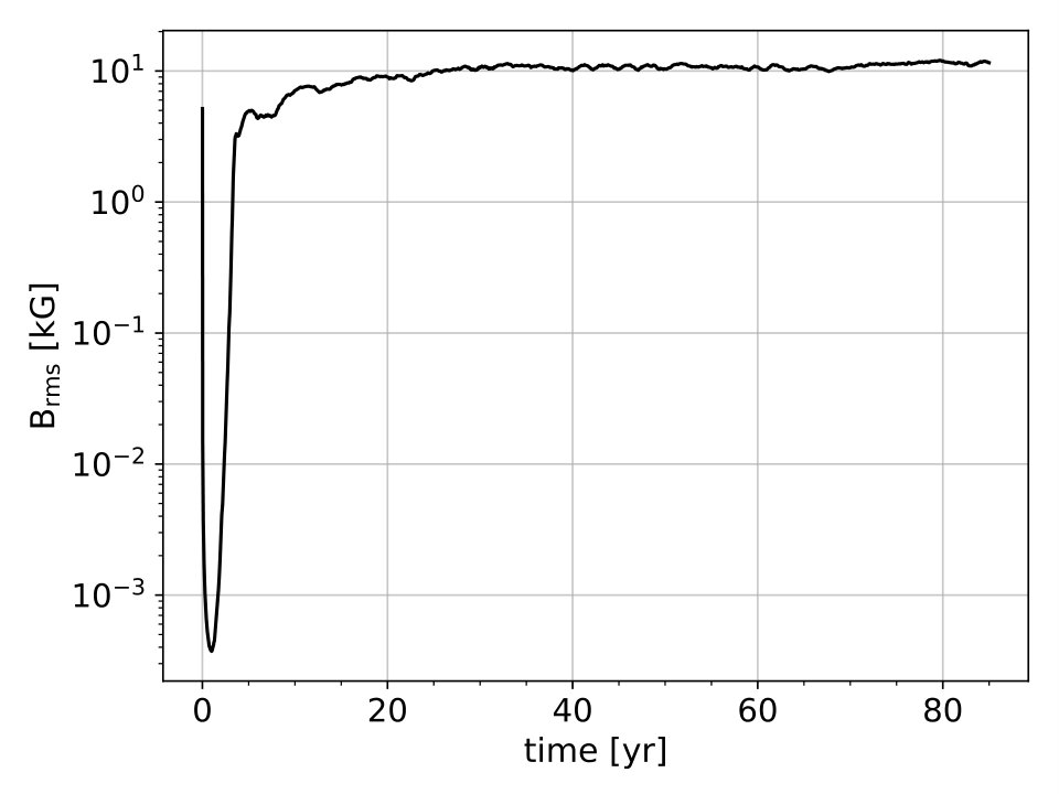 Figure 1
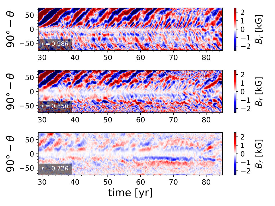 Figure 2
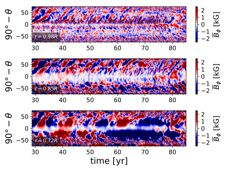 Figure 3
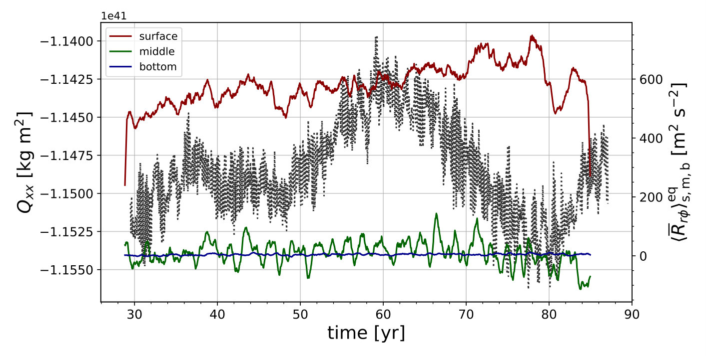 Figure 4
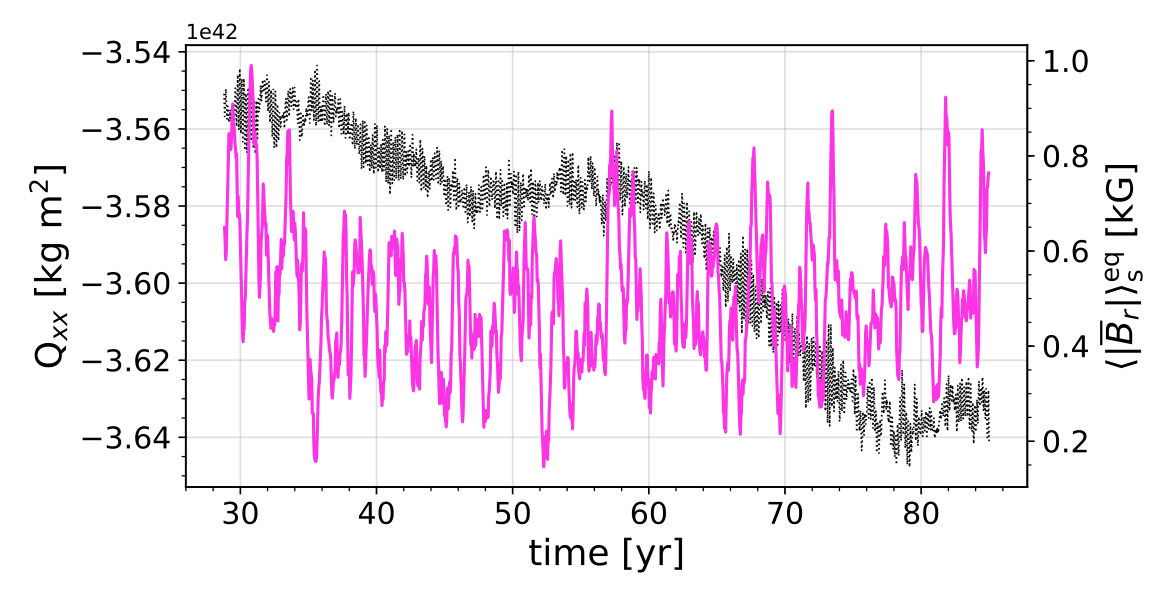 Figure 5
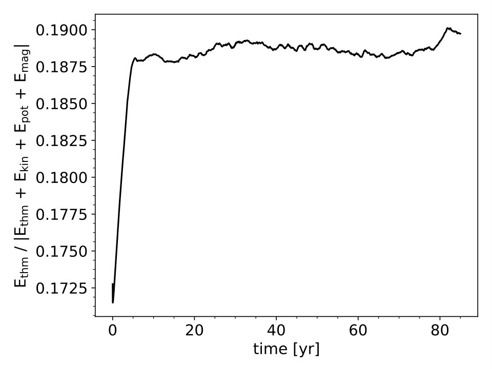 Figure 6
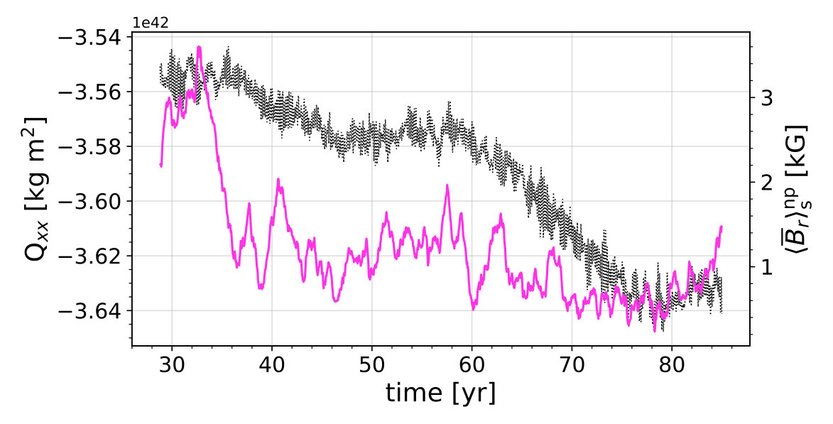 Figure 7
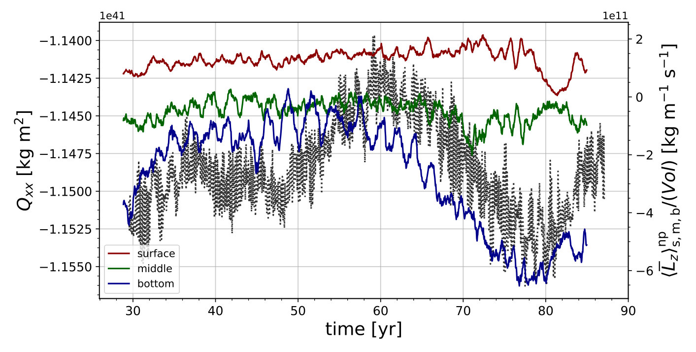 Figure 8
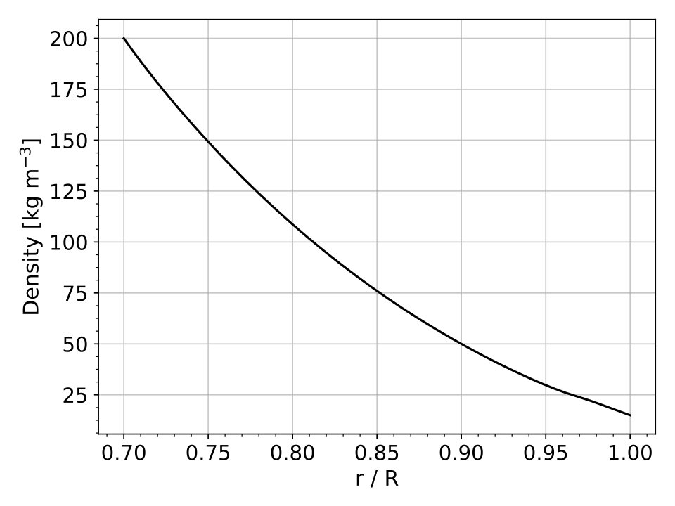 Figure 9
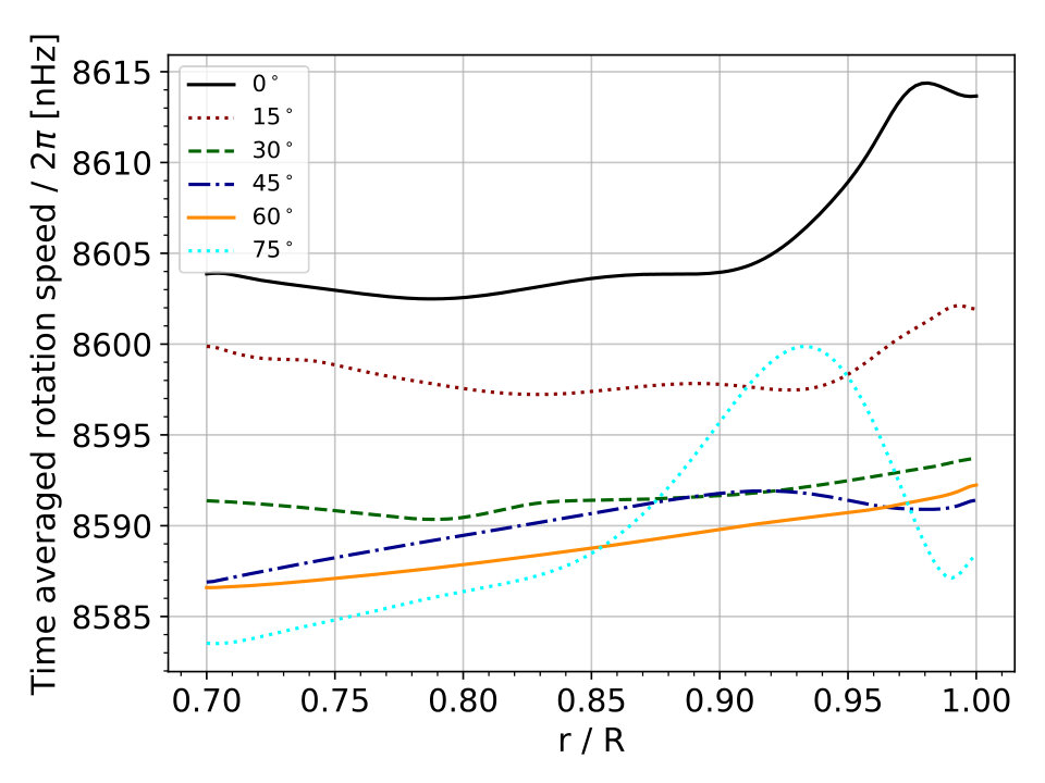 Figure 10
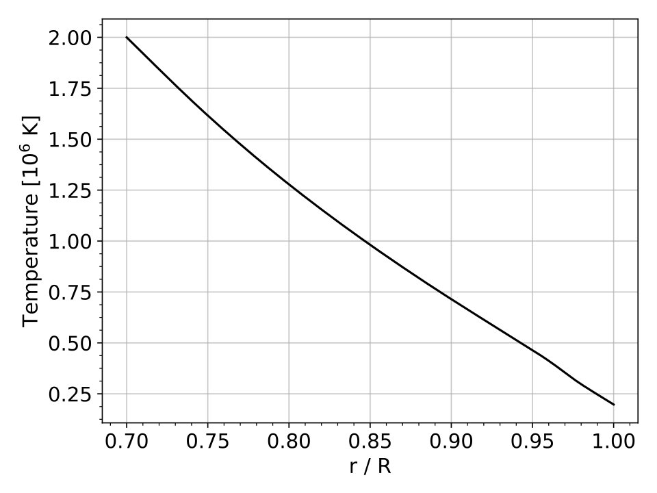 Figure 11
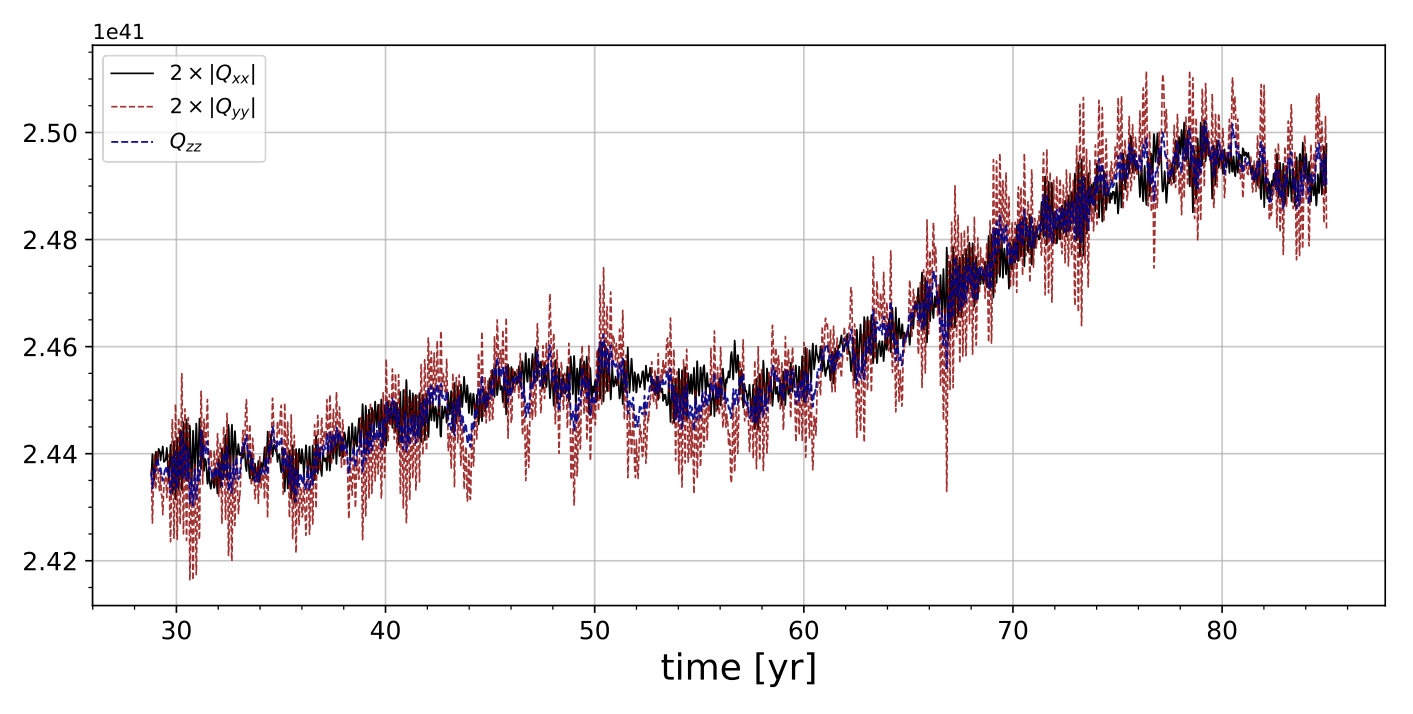 Figure 12
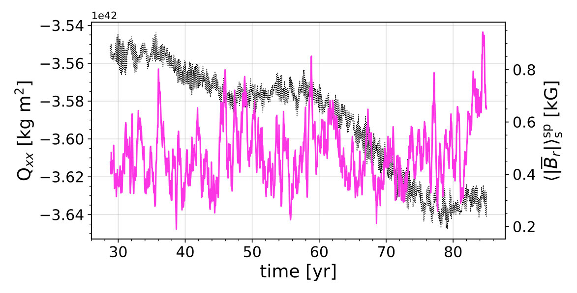 Figure 13
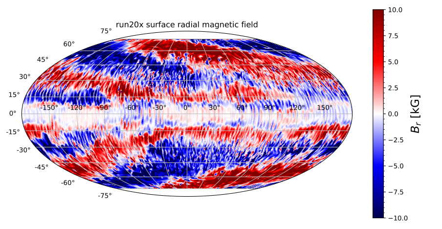 Figure 14
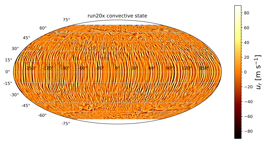 Figure 15
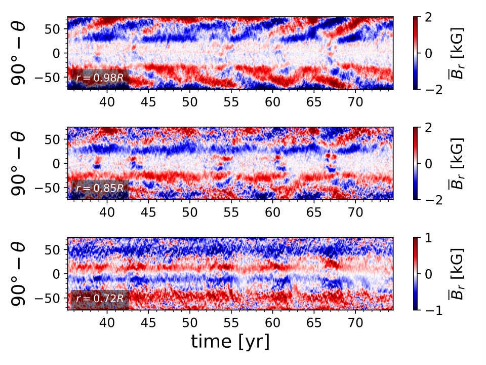 Figure 16
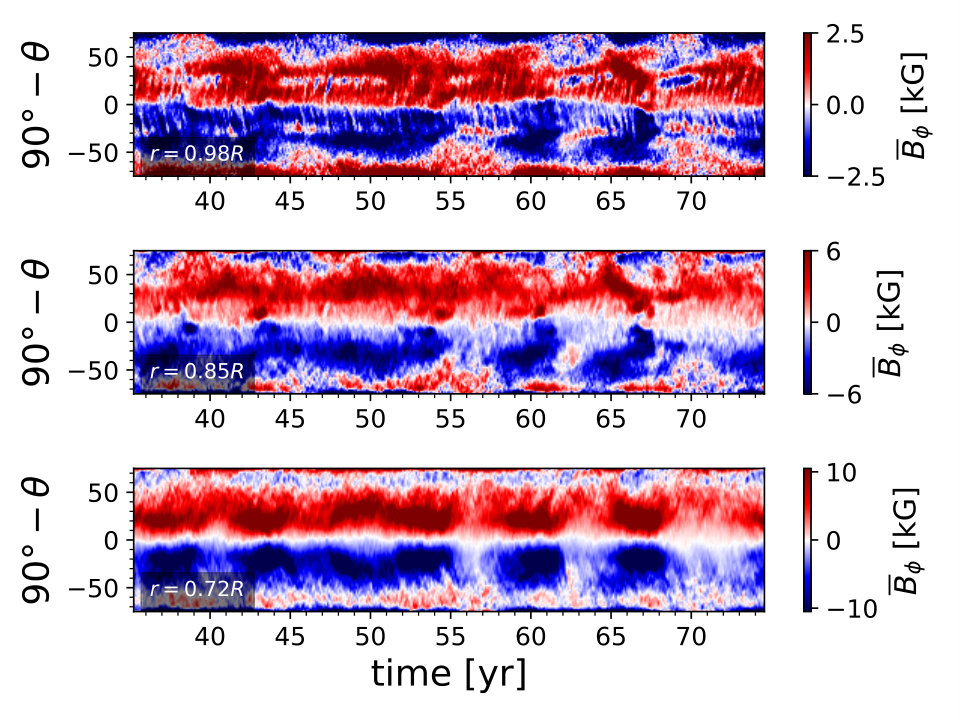 Figure 17
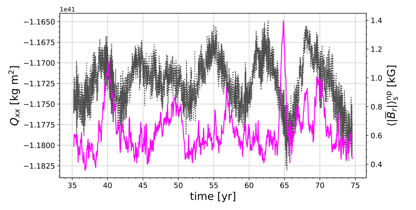 Figure 18
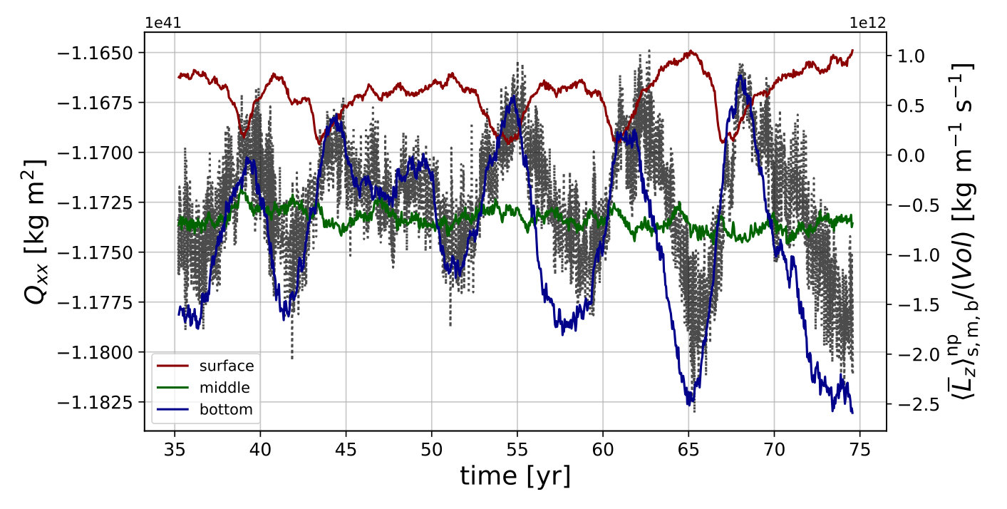 Figure 19
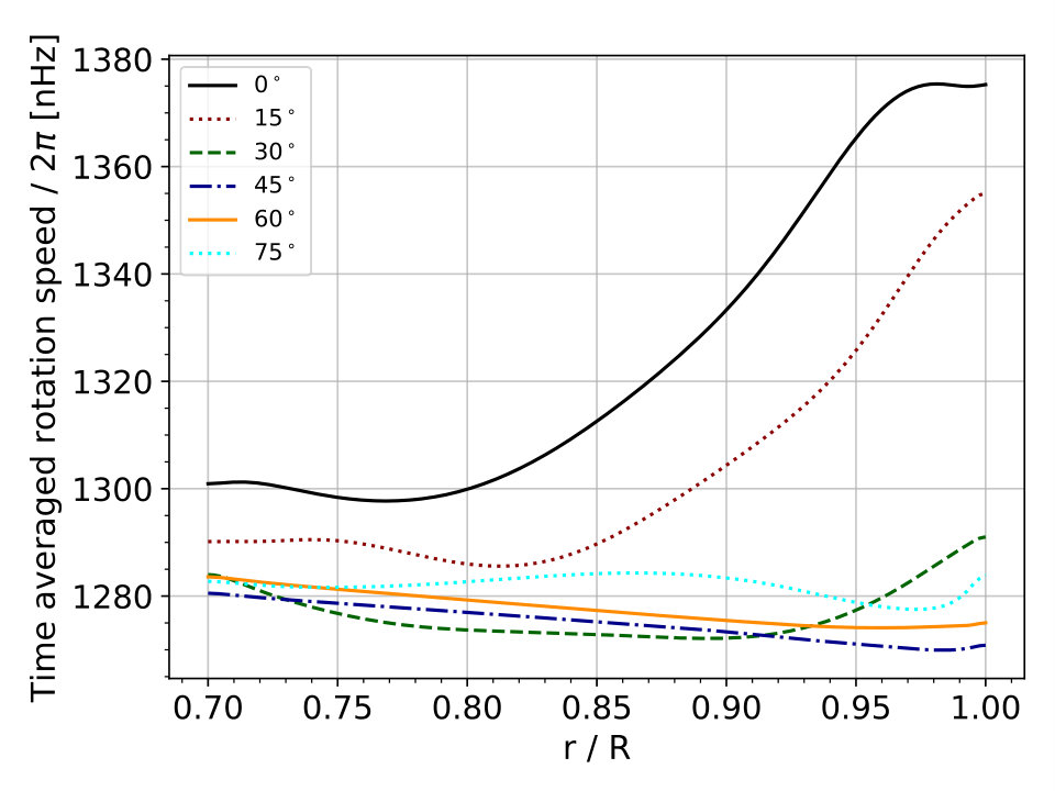 Figure 20
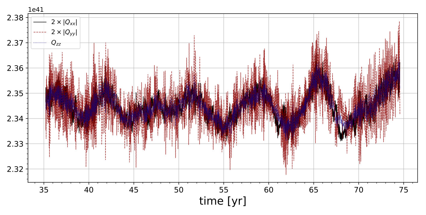 Figure 21
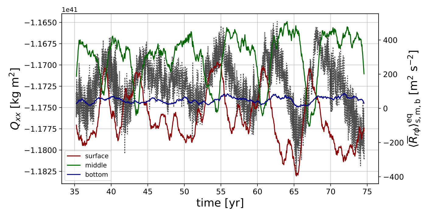 Figure 22
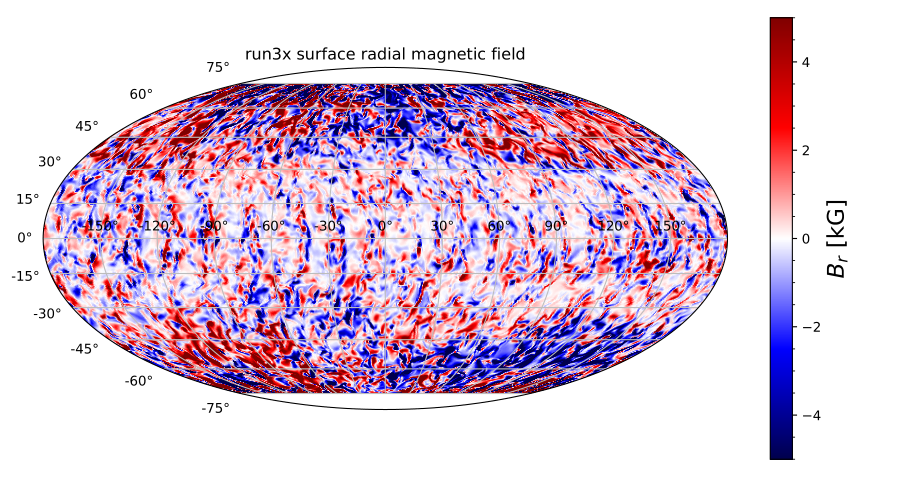 Figure 23
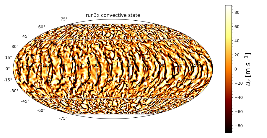 Figure 24
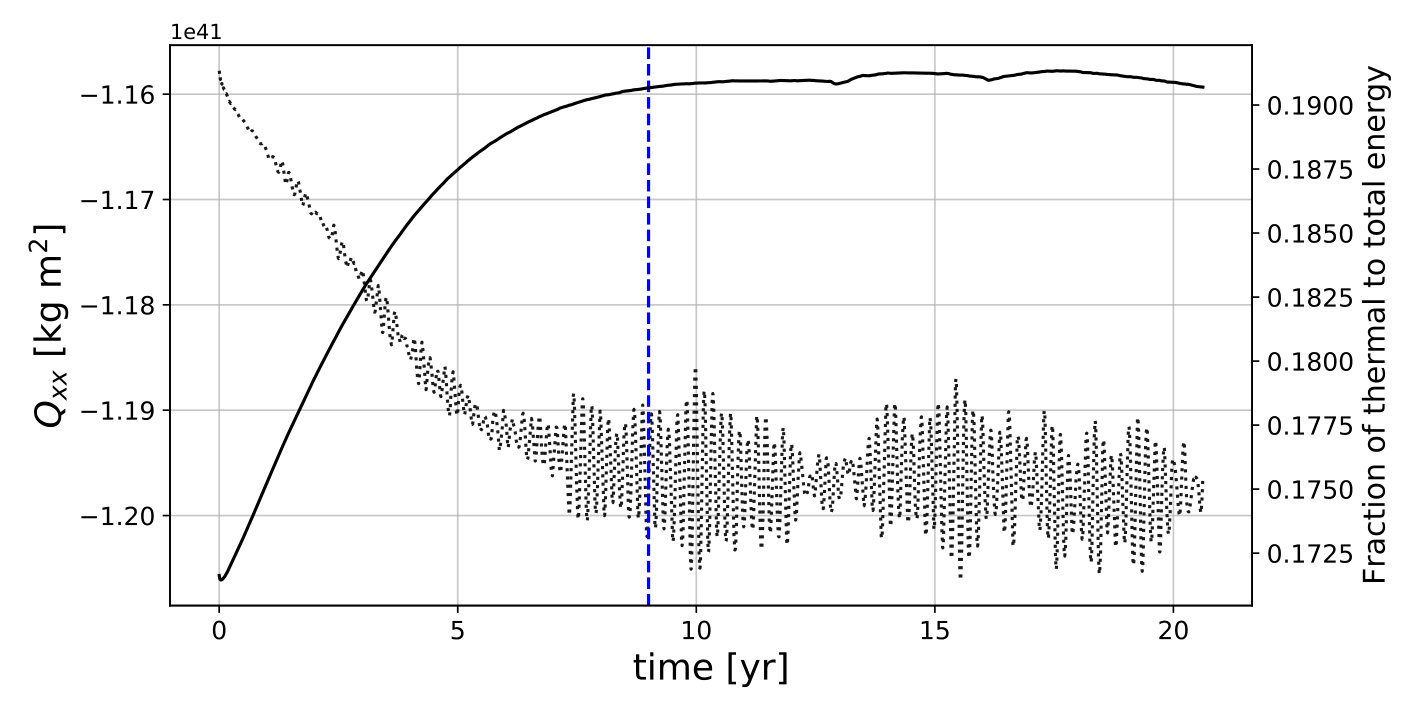 Figure 25
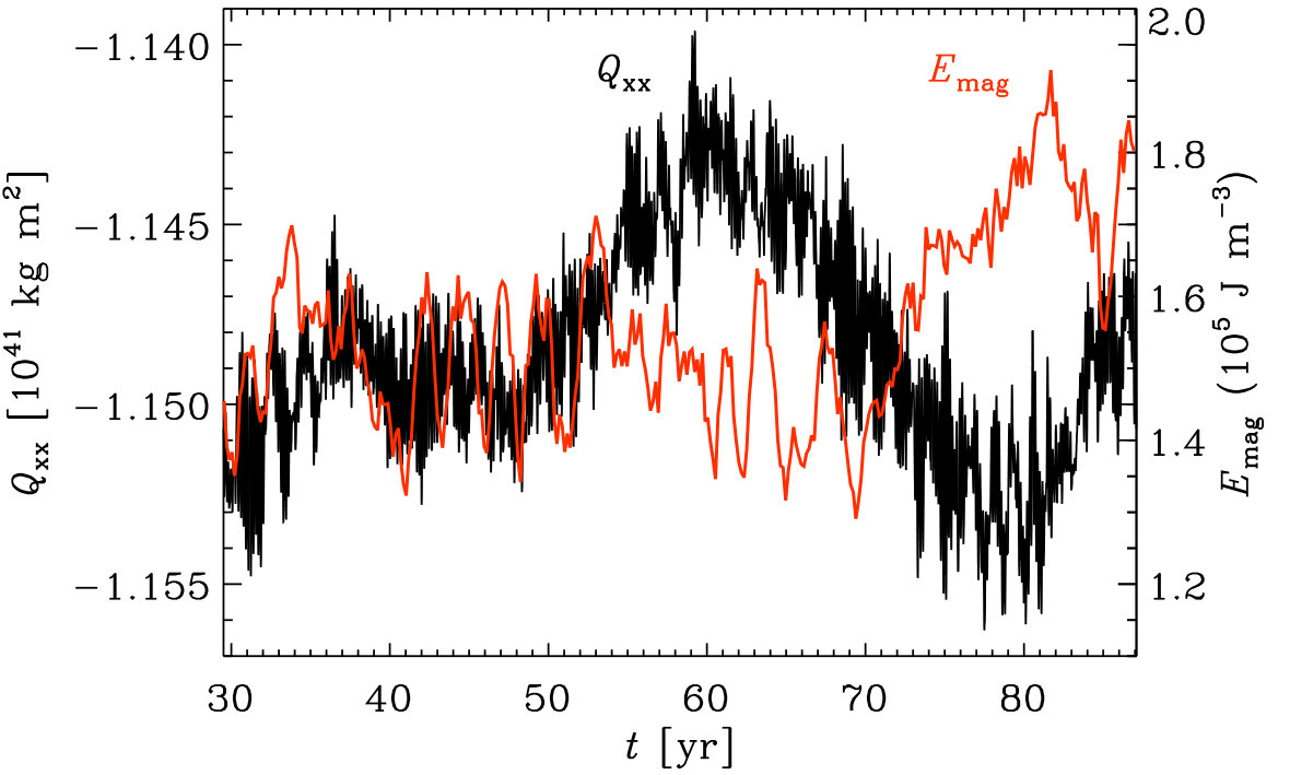 Figure 26
 Figure 27
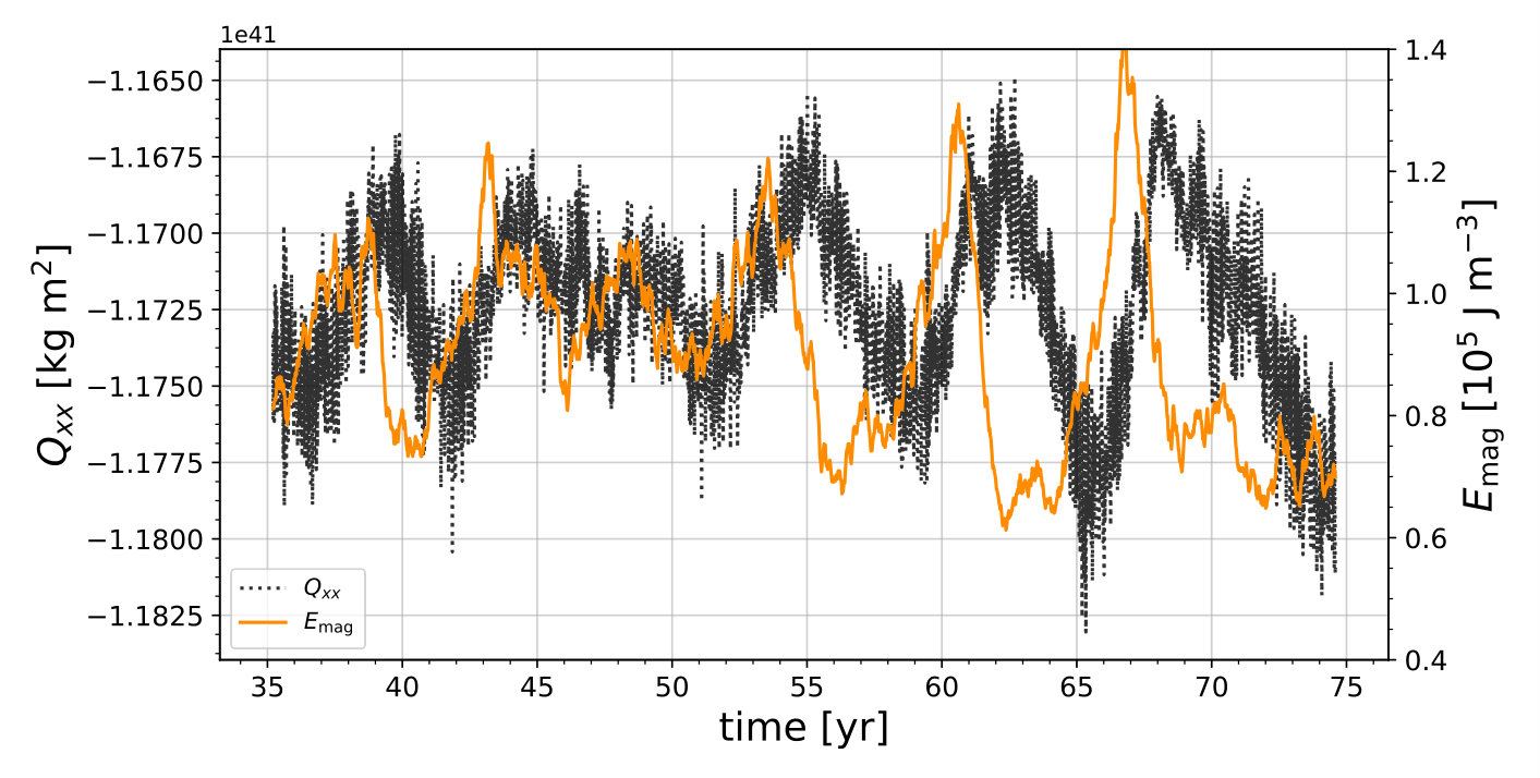 Figure 28
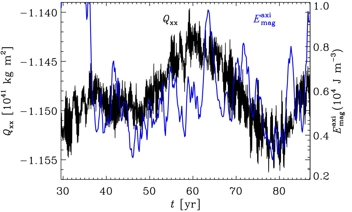 Figure 29
 Figure 30
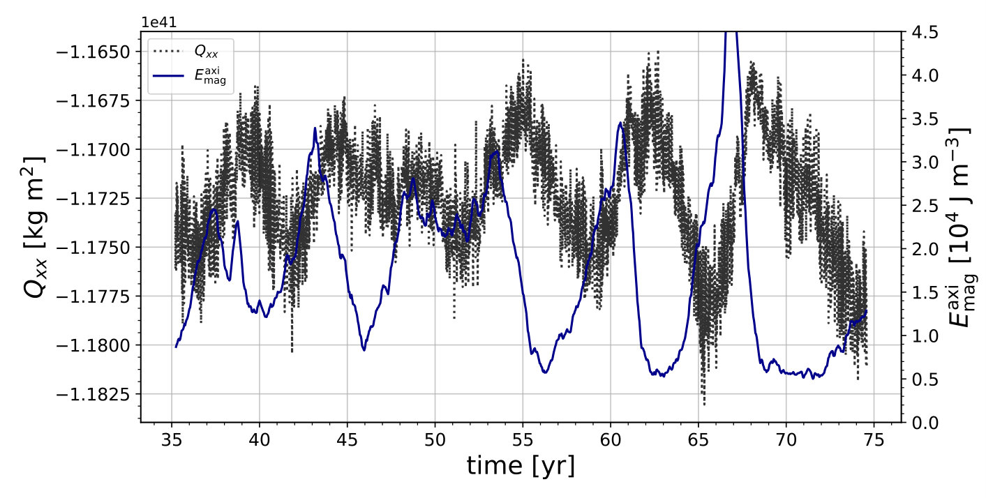 Figure 31
 Figure 32
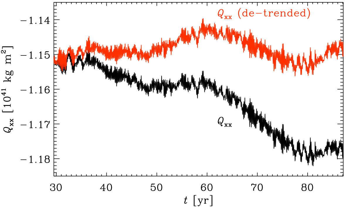 Figure 33
Peer Reviews
No public reviews on file for this paper yet. If you reviewed it on a platform where reviews are public (OpenReview, ICLR, NeurIPS, ICML), you can paste yours below so the community can read it here.
Videos
No videos yet. Explain this paper in a talk, walkthrough, or lecture? Add one.
Magneto-hydrodynamical origin of eclipsing time variations in post-common-envelope binaries for solar mass secondaries
Felipe H. Navarrete,1 Dominik R.G. Schleicher,1 Petri J. Käpylä,2,3 Jennifer Schober,4Marcel Völschow,5 Ronald E. Mennickent1
1Departamento de Astronomía, Facultad Ciencias Físicas y Matemáticas, Universidad de Concepción, Av. Esteban Iturra
s/n Barrio Universitario, Casilla 160-C, Concepción, Chile
2Fakultät für Physik, Georg-August-Universität Göttingen, Friedrich-Hund-Platz 1, 37077 Göttingen, Germany
3ReSoLVE Centre of Excellence, Department of Computer Science, Aalto University, PO Box 15400, FI-00076 Aalto, Finland
4Laboratoire d’astrophysique, Observatoire de Sauverny, CH - 1290 Versoix, Switzerland
5Hamburg Observatory, Hamburg University, Gojenbergsweg 112, 21029 Hamburg, Germany E-mail: [email protected]
(Accepted XXX. Received YYY; in original form ZZZ)
Abstract
Eclipsing time variations have been observed for a wide range of binary systems, including post-common-envelope binaries. A frequently proposed explanation, apart from the possibility of having a third body, is the effect of magnetic activity, which may alter the internal structure of the secondary star, particularly its quadrupole moment, and thereby cause quasi-periodic oscillations. Here we present two compressible non-ideal magneto-hydrodynamical (MHD) simulations of the magnetic dynamo in a solar mass star, one of them with three times the solar rotation rate (“slow rotator”), the other one with twenty times the solar rotation rate (“rapid rotator”), to account for the high rotational velocities in close binary systems. For the slow rotator, we find that both the magnetic field and the stellar quadrupole moment change in a quasi-periodic manner, leading to O-C (observed - corrected times of the eclipse) variations of s. For the rapid rotator, the behavior of the magnetic field as well as the quadrupole moment changes become considerably more complex, due to the less coherent dynamo solution. The resulting O-C variations are of the order s. The observed system V471 Tau shows two modes of eclipsing time variations, with amplitudes of s and s, respectively. However, the current simulations may not capture all relevant effects due to the neglect of the centrifugal force and self-gravity. Considering the model limitations and that the rotation of V471 Tau is still a factor of 2.5 faster than our rapid rotator, it may be conceivable to reach the observed magnitudes.
keywords:
dynamo – methods: numerical – MHD – binaries: eclipsing – stars: rotation
††pubyear: 2015††pagerange: Magneto-hydrodynamical origin of eclipsing time variations in post-common-envelope binaries for solar mass secondaries–Magneto-hydrodynamical origin of eclipsing time variations in post-common-envelope binaries for solar mass secondaries
1 Introduction
Post-common-envelope binaries (PCEBs) are close binaries that consist of a low-mass main-sequence star and a white dwarf (WD). Such systems are expected to form when the more massive component evolves until its surface extends beyond the outer Lagrangian point and eventually engulfs its companion (Paczynski, 1976). Then the less massive star experiences friction and deposits orbital energy and angular momentum into the common envelope (CE). It spirals inwards until the envelope is expelled due to the energy transfer, leaving a close binary, typically consisting of an M dwarf (dM) or a subdwarf and a white dwarf (see e.g., Parsons et al., 2013). The CE model has been revised and extended by various authors, including Meyer & Meyer-Hofmeister (1979); Iben & Livio (1993); Taam & Sandquist (2000); Webbink (2008) and Taam & Ricker (2010).
For about of these systems, eclipsing time variations have been observed (e.g. Zorotovic & Schreiber, 2013; Bours et al., 2016). The variations occur on rather long timescales of the order of years or more. Two possible interpretations of these variations are commonly discussed in the literature: The first is the presence of a third body, i.e. a planet or a brown dwarf, which would cause apparent eclipsing time variations due to the light-travel time (LTT) effect, i.e. the change in the light travel time to the observer due to the change of distance as the PCEB rotates around the common center of mass (e.g. Beuermann et al., 2010; Beuermann et al., 2013). Clearly, this effect requires rather massive planets (, where is the mass of Jupiter) on extended orbits (AU) to produce significant variations. Alternatively, such variations may also be produced through the Applegate mechanism (Applegate, 1992), which will be described in further detail below.
If the LTT is adopted, the eclipsing time variations imply the presence of two planets with masses of and and semi-major axis of AU and AU, respectively, in the system NN Ser (Beuermann et al., 2010; Beuermann et al., 2013) which often serves as a reference system for typical PCEBs. Beuermann et al. (2013) demonstrated the dynamical stability of these orbits, which was independently confirmed by Horner et al. (2012). However, when the additional data by Bours et al. (2016) are considered, they require an extra quadratic term in the expression for the eclispsing times if they want to maintain the planet solution. The physical origin of such an additional term is however unclear. In case of the system HW Vir, a two-planet solution appears to be secularly stable (Beuermann et al., 2012). A final conclusion on the stability of orbits in Hu Aqr is still pending (Goździewski et al., 2012; Hinse et al., 2012; Bours et al., 2014; Goździewski et al., 2015), and similarly for QS Vir (Parsons et al., 2010b). In the case of the system V471 Tau, the proposed third body has been searched via Direct Imaging, but has not been found (Hardy et al., 2015). Using the orbital period of the system (12.5-hr) and the spin period (9.25-min) of the WD as two independent clocks, Vanderbosch et al. (2017) have concluded that a third body interpretation cannot adequately explain the nature of this system.
If the planets in NN Ser are real, they should also be dynamically young, as the white dwarf has an age of only yrs (Parsons et al., 2010a). While their existence is highly speculative, they have at least two possible origins. The so-called first-generation scenario proposes that they formed together with the binary and then survived the common envelope phase, while the second-generation scenario implies that they formed through the material ejected during the common envelope phase. A hybrid scenario may be also possible, with accretion of the ejected gas onto already existing planets. Several studies have been carried out on this matter (e.g., Völschow et al., 2014; Schleicher & Dreizler, 2014; Bear & Soker, 2014), though it is currently difficult to draw any final conclusions.
The other possible explanation of the eclipsing time variations is magnetic activity. Historically, in particular the Applegate mechanism (Applegate, 1992) has been a relevant scenario, in which the magnetic activity of the secondary stars leads to a redistribution of the stellar angular momentum, thus changing its gravitational quadrupole moment. This in turn produces a variation of the binary separation. The original Applegate model has been improved by several authors. For instance, Lanza & Rodonò (1999) improved the model by adopting a consistent description of stellar virial equilibrium. Brinkworth et al. (2006) extended the model introducing a finite shell formalism, considering the exchange of the angular momentum between the shell and the core. Völschow et al. (2016) examined their model in more detailed and applied it to a sample of close binary systems (predominantly PCEBs), showing that the Applegate mechanism is a viable process in the shortest and most massive binary systems. The corresponding model has been made public through the Applegate calculator111Applegate calculator: http://theorygroup-concepcion.cl/applegate/index.php, and shows that the mechanism is favored in particular for rapidly rotating systems (Navarrete et al., 2018).
In addition to the finite shell model, Lanza & Rodonò (2004) and Lanza (2005) presented a one-dimensional framework based on the angular momentum transport equations, using simplifying assumptions of magneto-hydrodynamical (MHD) turbulence and the mean magnetic field. We have extended this framework in Völschow et al. (2018), considering in particular time-dependent hydrodynamic and magnetic fluctuations assuming a magnetic activity cycle, as well as a superposition of different modes. For typical RS Canum Venaticorum (RS CVn) systems, which are detached binaries typically composed of a chromospherically active G or K star, the expected eclipsing time variations are however two orders of magnitude lower than observed. The most promising Applegate candidates are post-common-envelope binaries with secondary masses of M⊙ (Völschow et al., 2018), as these produce more energy through nuclear burning and can thus more easily redistribute angular momentum as required by the Applegate mechanism, while simultaneously not being critically affected by the presence of a radiative core.
The presence of magnetic activity should be expected in these systems due to the convective envelopes of the secondaries and their rapid rotation. A corresponding dynamo model has been put forward by Rüdiger et al. (2002). Observationally, magnetic activity has been inferred on many occasions. In the case of V471 Tau, it has been probed via photometric variability, flaring events and H emission along with a strong X-ray signal (Kamiński et al., 2007; Pandey & Singh, 2008). For DP Leo, magnetic activity has been revealed through X-ray observations (Schwope et al., 2002). In the system QS Vir, it is indicated via detections of Ca II emission and Doppler imaging (Ribeiro et al., 2010), as well as observed coronal emission (Matranga et al., 2012). In case of HR 1099, a 40 year X-ray light curve suggesting a long-term cycle was recently compiled by Perdelwitz et al. (2018), and similar studies have been pursued via optical data (e.g., Donati et al., 2003; Lanza et al., 2006; Berdyugina & Henry, 2007; Muneer et al., 2010).
While magnetic activity is potentially relevant to explain the origin of the eclipsing time variations, its effects on the stellar structure so far have only been explored via finite shell or 1D models, in both of which the presence of a dynamo was externally imposed. However, a self-consistent modeling of the dynamo and its interaction with the stellar structure may be crucial, and is only possible within 3D magneto-hydrodynamical (MHD) simulations. While stellar dynamo models have previously been pursued (see e.g. Yadav et al., 2016), the latter was done in the anelastic limit, which does not allow to explore the effect of the dynamo onto the stellar structure. Here as a first step, we will employ a fully compressible setup developed by Käpylä et al. (2013) for a solar mass star although with rotation rates exceeding the solar one. These models allow the quantification of changes in stellar structure due to the dynamo. While solar mass stars are not very common in post-common-envelope systems, they do occasionally occur, as for instance the secondary of V471 Tau has a mass of M⊙ (Zorotovic & Schreiber, 2013), and is thus still consistent with being a solar mass star. Independently, we of course stress that this is an exploratory study that should be extended to stars of different masses as well.
In section 2, we will briefly introduce the Pencil Code222https://github.com/pencil-code/ (Brandenburg & Dobler, 2002; Brandenburg, 2003) as well as the setup employed here, which is based on previous developments by Käpylä et al. (2013). In these simulations, the Rayleigh number, which describes the ratio of the time scale for thermal transport via diffusion to the time scale for thermal transport via convection, is however much smaller than in reality due to the higher diffusivities required for numerical stability, see detailed discussions in Käpylä et al. (2013) and Kupka & Muthsam (2017). Another caveat of fully compressible simulations of solar-like stars is that the low Mach number in the deep parts of the convection zone necessitates a very short time step and that the thermal relaxation occurs in the Kelvin–Helmholtz timescale which is of the order of () years for the whole Sun (solar convection zone) (see, e.g. Kupka & Muthsam, 2017). Thus, to bring the dynamic and acoustic timescales closer to each other and to shorten the Kelvin–Helmholtz timescale, the energy flux needs to be enhanced (see also Brandenburg et al., 2005). To compensate for this and to obtain a comparable rotational influence on the flow as in real stars, which is the key factor determining their dynamo properties, the angular velocity needs to be increased proportional to one third power of the increase of the energy flux (see a detailed description in Käpylä et al., 2019). For this reason, the effect of the centrifugal force has been omitted in this formulation of the Navier-Stokes equation, as the resulting centrifugal force would be too high, thereby significantly altering the hydrostatic balance (Käpylä et al., 2011, 2013). With this in mind, we note that our simulations present only a first step, where the redistribution of material can be explored for instance due to meridional flows, and we will not probe the effect originally proposed by Applegate (1992). Nevertheless, the occurence of quadrupole moment variations even in the absence of the centrifugal force term is a central outcome of the simulations. The results of our simulations are presented in section 3, including a hydrodynamical reference run and two MHD simulations. Our discussion and conclusions are presented in section 4.
2 Methods
2.1 Pencil Code
The Pencil code (Brandenburg & Dobler, 2002; Brandenburg, 2003) is a finite-difference code written in Fortran 95. It uses sixth-order spatial derivatives and a third-order Runge-Kutta time integrator scheme, which makes the code particularly useful for studying weakly compressible turbulent flows. For the timestepping, a high-order scheme is implemented in order to reduce amplitude errors and to allow longer time steps, which is the RK-2N Runge-Kutta scheme (Williamson, 1980), where the “2N" stands for its memory consumption of two chunks. The time step is specified by the Courant time step. The Message passing interface (MPI) is used for parallelization.
2.2 The model
The model we use here is based on those used by Cole et al. (2014) and Viviani et al. (2018) and is described here for completeness. The computational domain is spherical but without the poles, which allows to reach a higher spatial resolution but at the cost of omitting connecting flows across the poles and introducing artificial boundaries at high latitudes. The domain denotes radial, colatitudinal, and longitudinal directions. The radius extends from (the bottom of the convection zone) to , where is the solar radius; goes from to , and from [math] to . The corresponding grid resolution is . We employ the compressible non-ideal MHD equations in the following form:
[TABLE]
where is the magnetic vector potential, and are the velocity and magnetic field, is the electric current density with being the vacuum permeability. is the convective derivative, is the density, and
[TABLE]
and
[TABLE]
are the radiative and subgrid scale (SGS) fluxes. The former accounts for the flux coming from the radiative core and the latter is added to stabilize the scheme and to account for the unresolved turbulent transport of heat. and are the radiative heat conductivity and and turbulent entropy diffusivity, respectively. is the specific entropy, is the pressure, and is temperature. Furthermore, the system of equations (1)–(4) is closed by assuming an ideal gas law,
[TABLE]
where is the ratio of specific heats at constant pressure and volume, and is the specific internal energy. is the traceless rate-of-strain tensor
[TABLE]
where semicolons denote covariant differentiation. is the gravitational acceleration with being the gravitational constant, the stellar mass, and the radial unit vector. The stellar rotation vector is given as . As already discussed in the introduction, the formulation of the Navier-Stokes equation employed here does not include the centrifugal force term, which would be unrealistically high (see Käpylä et al., 2011, 2013, 2019, for details).
2.3 Initial and boundary conditions
The initial state is isentropic with a temperature gradient given as
[TABLE]
where is the polytropic index for adiabatic stratification. The fixed values that define a simulation are (i) the energy flux at the bottom,
[TABLE]
where is the radiative conductivity, is a constant (Käpylä et al., 2013), and
[TABLE]
Here at the bottom and at the surface. This choice is made to ensure that the radiative flux at the bottom is solely responsible for supplying energy into the system and that convection transport essentially the total flux in the bulk of the convection zone (CZ). The remaining parameters of the model are (ii) the angular velocity , (iii) viscosity , (iv) magnetic diffusivity , and (v) turbulent heat conductivity and its radial profile (see Käpylä et al., 2013). The turbulent velocity and magnetic fields are initialized with small-scale low amplitude Gaussian noise perturbations.
2.3.1 Radial boundary
The radial boundaries are assumed to be impenetrable and stress-free, i.e at :
[TABLE]
The bottom is assumed to be a perfect conductor with
[TABLE]
and at the top the magnetic field is radial
[TABLE]
The value of is fixed at the bottom and the upper radial boundary uses a black body condition
[TABLE]
where is a modified value of the Stefan-Bolzmann constant (see Käpylä et al., 2013).
2.3.2 Latitudinal boundary
The latitudinal boundary is also assumed to be stress-free at °, 165°
[TABLE]
and a perfect conductor
[TABLE]
Density and entropy are assumed to have zero first derivative on both boundaries, thus suppressing heat fluxes through them.
2.4 Quadrupole moment and its scaling
The quadrupole tensor is defined as
[TABLE]
where denotes the trace and is the tensor of inertia
[TABLE]
where refer to Cartesian coordinates.
As already mentioned in the introduction, the stellar luminosity is enhanced due to numerical constraints (see Brandenburg et al., 2005; Käpylä et al., 2019). As a result, the energy flux coming from the bottom is much higher than in the Sun. The ratio of fluxes in the present case is
[TABLE]
The increased flux implies that the fluctuations of other quantities are correspondingly enhanced. The fluctuation of the pressure can be written as
[TABLE]
where the subscript indicates constant entropy and where is the sound speed. Furthermore, variations in pressure scale as
[TABLE]
Equating (26) and (27) we obtain
[TABLE]
Here Ma is the Mach number, which scales as (e.g. Käpylä et al., 2019; Käpylä, 2019)
[TABLE]
and thus,
[TABLE]
All of the numbers given in sections 3.3.4 and 3.4.4 have been rescaled in this fashion, which corresponds a factor of , i.e.
[TABLE]
where the subscript ‘sim’ denotes the estimated quadrupole moment obtained in the simulations.
Furthermore, we define the Taylor, Coriolis, fluid and magnetic Reynolds, and SGS and magnetic Prandtl numbers as
[TABLE]
where is the volume-averaged root-mean-square velocity, is an estimate of the wavenumber of the largest eddies, and is the SGS entropy diffusion at .
3 Results
In this section, we present our main results obtained from the numerical simulations. In subsection 3.1, we introduce the notation used throughout the paper and discuss the overall properties of our simulations. We first discuss a pure hydrodynamical reference run in subsection 3.2 to demonstrate that the long-term modulation of the quadrupole moment must have a magneto-hydrodynamical origin. We then present two MHD models, a slow rotator (3 times solar rotation, days) and a fast rotator (20 times solar rotation, days) in subsections 3.3 and 3.4. These values were chosen as the rotation rate in PCEBs is considerably enhanced compared to isolated stars, with a rotation period in V471 Tau of about d (Zorotovic & Schreiber, 2013).
3.1 Notation and General Properties
We label the two MHD simulations according to their rotation rates, namely run3x for the 3 times solar rotation, and run20x for the 20 times solar rotation rate. Quantities with an overline indicate an average over the azimuthal angle; e.g. indicates an average of the component of over and is given by
[TABLE]
Other averages are presented inside angular brackets with sub- and superscripts. For example, indicates an average of in regions denoted with and . The subscript indicates the depth at which the quantity of interest is taken and the superscript indicates the latitude where the average is further calculated with the following rules:
[TABLE]
where
[TABLE]
and
[TABLE]
where is colatitude. So for example, indicates the average of the azimuthally-averaged over , i.e. the equatorial, near the surface of the computational domain.
Typical density and temperature profiles are shown in Figure 1, corresponding to the final state of run20x.
The density at the bottom is 181.8 kg m*-3* and 13.6 kg m*-3* at the surface, where bottom and surface are evaluated following the definition in (38) and (40). This corresponds to a density
[TABLE]
The temperature profile is shown in the lower panel of Figure 1. The temperature at the bottom is set to be the same as the temperature at the bottom of the CZ in the Sun, namely K, and decreases towards a value of K at the surface.
The time-averaged angular velocity is shown from six latitudes from run3x in the top panel of Figure 2. Overall the rotation is faster at the equator than at high latitudes, but we often observe an increase in the angular velocity at the latitude boundaries (see the cyan-dotted lines in Fig. 2). This is likely an artefact due to the impenetrable latitude boundary. In the lower panel of Figure 2, we show the time-averaged rotation profile for run20x. The difference in the rotation rates between high latitudes and the equator is significantly smaller than in the slower rotator. The decrease of differential rotation as the overall rotation rate is increased is consistent with earlier studies (e.g. Viviani et al., 2018).
At the beginning, the simulations first have to go through a relaxation phase during which thermal and magnetic saturation is established. The description that follows corresponds to run20x, but is qualitatively the same for run3x. There are two conditions that need to be fulfilled before analyzing the results and deriving astrophysical implications for PCEB systems:
On the one hand, the system has to reach dynamo saturation, which is shown in Figure 3, where we plot the root-mean-squared magnetic field for run20x. The seed magnetic field first decays because most of the initial magnetic energy is contained on the small scales which is quickly dissipated (Dobler et al., 2006). Furthermore, it takes susbtantial time for convection and large-scale flows to develop that lead to dynamo action. Subsequently, the magnetic field grows exponentially during the next three years during the kinematic stage. This growth starts to slow down in the non-linear regime until it reaches the saturation stage after about years.
The system has to also reach thermal equilibrium, which is shown in Figure 4, where we plot the fraction of thermal to total energy. The only energy source in the simulations is the energy injected from the bottom of the convection zone. While most of this energy is transported to the surface by convection, a fraction is deposited in the thermal reservoir of the convection zone until equilibrium between energy input and output is achieved. This is manifested by an increase of the thermal energy in the present case. Thermal evolution after roughly 8 years is slow and the system is sufficiently close to thermal saturation to be used for statistical analysis of the data.
3.2 Purely hydrodynamical simulation
Here we present a pure hydrodynamical reference run with 20 times solar rotation. This serves essentially for comparison with the MHD simulations, to demonstrate that long-term variations only occur in simulations that include magnetic fields.
Figure 5 shows the change of the gravitational quadrupole moment in the dotted line, together with the thermal energy as a fraction of the total energy of the system as solid line.
Here we can see very high frequency oscillations with a period of 0. years. This is very close to an average sound-crossing time , which we calculate as
[TABLE]
where is the radial extent of the simulations, and corresponds to the sound-speed, , averaged over the radial direction. The sound-speed is calculated as
[TABLE]
where the subscript ‘s’ indicates the derivative is taken at constant entropy. Thus the high frequency oscillations have a purely hydrodynamical origin.
3.3 The case of the slow rotator (run3x)
We first investigate the evolution of a simulation with three times solar rotation. This case is characterised by , , , , and . Simulations with similar parameters were also explored by Viviani et al. (2018) for the stellar dynamo but they have not explored the implications on the stellar structure.
3.3.1 Overview of convective and magnetic states
To illustrate the general structure, we first examine a snapshot at the end of the simulation. Figure 6 shows a Mollweide projection (an equal-area map projection also known as homolographic projection) of the near surface radial velocity. The colorbar is cut at m s*-1* to improve visualization. The velocity field does not show clear signs of large-scale structures.
At the equator we see elongated cells (sometimes called “banana cells”). Their existence is due to the influence that rotation has on the flow (see Busse, 1970). At higher latitudes the the banana cells disappear, and the effect of rotation is to give rise to more symmetric and smaller cells (see, e.g. Chandrasekhar, 1961). It should be noted that these cells are much larger than those observed in the Sun which is due to the much lower density stratification in the simulations. The mean radial velocity is 60 m s*-1*, while the extrema can reach 1000 m s*-1*.
In Figure 7 we plot the near surface radial magnetic field at the end of the simulation. The colorbar is cut at kG to improve visualization. The magnetic field strength at the equator is weaker than at high latitudes, and a clear non-axisymmetric component is observed. The mean magnetic field strength is 2.5 kG and the extrema are 90 kG. The sizes of the magnetic structures is much larger than, e.g., sunspots. This is due to the fact that the current simulations lack the resolution to capture the small-scale granulation near the surface and the physics leading to spot formation.
3.3.2 Overview of the magnetic field evolution
We start the analysis by examining the dynamo solution of the slow rotator. Figure 8 shows the evolution of the mean toroidal magnetic field (butterfly diagram) of run3x at three depths. At the northern hemisphere there is an overall positive polarity whereas in the southern hemisphere the dominant polarity is negative. In each panel, the polarity near the latitude boundaries is opposite to the dominant polarity. Polarity reversals can be seen at high latitudes at the bottom of the convective region (third panel). In the middle (second panel), these reversals at the poles are more pronounced and thus easier to see whereas at the surface the reversals are not as clearly observed in the azimuthal field. Thus it appears that the axisymmetric part of the magnetic field consists of a dominant quasi-stationary component and a weaker quasi-periodic one, as also recently reported by Viviani et al. (2019). Meanwhile, the strength of the azimuthal magnetic field is varying quasi-periodically without polarity reversals near the equator. At the three reference depths there are episodes of decreased activity, for example at the equator during the time frames of 55 to 59 years and 62 to 66 years. The extrema at the bottom, middle, and surface are 20 kG, 7 kG, and 3 kG, respectively.
The evolution of the radial field is shown in Figure 9. At the bottom of the convective zone (bottom panel) the behaviour of is similar to the one described for the toroidal field at the surface. At low latitudes and towards the equator the magnetic field is positive (negative) at the northern (southern) hemisphere, and there are no clear signs of polarity reversals. In the middle of the convective region we start seeing hints of a poleward migrating dynamo wave (see second panel in Figure 9) at latitudes greater than in both hemispheres. Meanwhile, at mid-latitudes () a persistently negative (positive) magnetic field in the northern (southern) hemisphere is obtained with no migration. Near the equator, the mean radial magnetic field is weaker but with periods of increased strength at years. At the surface of the star (top panel) a dynamo wave is obtained with a poleward migration. At the equator the strength of is weaker with periods of increased strength at the same times as in the middle of the computational domain.
3.3.3 Origin of the quadrupole moment fluctuations
The time evolution of the diagonal elements of the quadrupole moment , and is shown in Fig. 10. While is positive, and are negative, and there is a difference of about a factor of in the components. Apart from that, their overall behavior is very similar, showing a quasi-periodic evolution with a period of around 8 years, and an amplitude of the order of kg m2 in the case of . For comparison, we also applied the semi-analytic model by Völschow et al. (2018), obtaining the same order of magnitude for the fluctuations. The system further shows the presence of short-term oscillations, which are also present in hydrodynamical runs (see Sect. 3.2). We will in the following take the component as a reference that we compare to other quantities, keeping in mind that the result would be similar for the other components as well.
We compare the evolution with the average radial magnetic field near the surface averaged over the northern hemisphere in Figure 11. We can see peaks of the magnetic field and how they relate to the quadrupole moment. The first peak of the magnetic field at years can be related to the minimum of at years. Then, the continuous increase in the magnetic field intensity from years to years is reflected in a decrease of starting at the 45 years mark to years. This shows the direct impact of magnetic field to the overall density distribution of the star. We also compare the evolution of directly with the evolution of the total and axisymmetric magnetic energies in Figure 12 top and bottom panels. Here we see a close anticorrelation between the magnetic energy and in both panels, and a time lag might also be present.
Now, we explore the correlation between the Reynolds stress tensor component , where primes denote fluctuations from azimuthal averages which are denoted by overbars, which is known to drive differential rotation (Rüdiger, 1989; Käpylä et al., 2016). This is shown in Figure 13. The stress at the surface (middle) of the computational domain is correlated (anticorrelated) with the quadrupole moment. The stress at the bottom is weak and with a small contribution and weak correlation to .
Finally, we study how the angular momentum , where is related to . In Figure 14, we plot the angular momentum per unit volume averaged over the northern hemisphere at the surface (red), middle (green), and bottom (blue). While the angular momentum itself will not directly affect the stellar structure through the centrifugal force, it changes due to the Reynolds stress and shows a strong correlation here with the change of the quadrupole moment.
From this figure we see that the outer layers carry less angular momentum than the inner ones, and at the surface there is an anti-correlation between the absolute value of and the absolute value of . The angular momentum at the surface further appears to be anti-correlated with the angular momentum in the middle and at the bottom, thus indicating an internal redistribution.
3.3.4 Gravitational quadrupole moment evolution
We return to Figure 10 to analyze the time evolution of quadrupole moment. We are interested in variations on timescales longer than the hydrodynamic oscillations with a period of 0.18 years, see Section 3.2. The variations in are not strictly periodic. For example, there is an episode between yr to yr where it takes clearly more time to reach a local maximum. Furthermore, reaches a global minimum at yr which is clearly lower than those that precede it. This behaviour is to be expected to a certain degree as the full set of MHD equations is highly non-linear. Overall, these fluctuations have a period of years and semi-amplitudes of kg m2.
Bearing in mind the necessary rescaling to obtain astrophysical values (see section 2.4) and that we are modeling a solar mass star, we can use the results from our simulations to estimate the impact in V471 Tau. Following Applegate (1992), the variations in the binary period are related to variations in the quadrupole moment via
[TABLE]
or,
[TABLE]
where and are the mass and radius of the magnetically active star, and is the binary separation. We take the semi-amplitude as
[TABLE]
and adopt a binary separation of 3.3 . This result is consistent with the semi-analytic model by Völschow et al. (2018), adopting fluctuations of about in the turbulence and magnetic field. We therefore obtain
[TABLE]
Furthermore,
[TABLE]
where is the modulation period of the diagram (see Applegate, 1992). Combining this equation with Equation (48) yields
[TABLE]
Marchioni et al. (2018) presented the most updated analysis of the eclipsing times of V471 Tau. The authors reported two period variations, one with 151 s and years. The other contribution has a semi-amplitude of 20 s and a modulation period of years. The semi-amplitude obtained from the simulations in this case is thus much lower than observed. However, we note that the rotation rate is different than in V471 Tau, and also the stellar mass may not be exactly the same. Indeed, more promising results will be obtained with the fast rotator in the next section.
3.4 The case of the fast rotator (run20x)
We now investigate the evolution of a simulation with twenty times solar rotation. This case is characterised by , , , , and . Also this simulation lies within the parameter regime explored by Viviani et al. (2018).
3.4.1 Overview of convective and magnetic states
Figure 15 shows the near-surface radial velocity from run20x. Also here, banana cells here are present at the equator, but with a decreased azimuthal extent in comparison to run3x. At higher latitudes the size of the convection cells is also reduced. This decreasing size of convection cells as the rotation increases is in accordance with linear stability analysis (e.g. Chandrasekhar, 1961) and earlier numerical simulations (e.g. Viviani et al., 2018). The average convective velocity is 19.4 m s*-1*, with extrema of 700 m s*-1* and m s*-1*.
Figure 16 shows the near-surface radial magnetic field at the end of run20x. The radial magnetic field differs from that of run3x in that it is stronger and more organized. The rms radial magnetic field is 4.5 kG, i.e. 1.8 times stronger than in run3x. The extrema are about 90 kG, as in run3x. These large-scale magnetic structures can cover the whole surface of the star. A possible explanation is that convection in the rapidly rotating run is less supercritical in terms of its Rayleigh number because the values of and remain the same as in run3x. Thus the flows and magnetic fields in run20x are more laminar than in run3x.
3.4.2 Overview of the magnetic field evolution
We follow here the same approach as in the case of the slow rotator. Figure 17 shows the time evolution of the mean toroidal magnetic field, i.e. butterfly diagram, at three depths labeled at the lower left corner of each panel. The mean magnetic field shows a more complex behavior than in run3x. At the bottom of the domain the dynamo solution is cyclic everywhere in the beginning. The maximum amplitudes are 12 kG. At later times there is a quasi-stationary axisymmetric magnetic field from 57 years to 76 years, covering most of the southern hemisphere. The dynamo solution at the middle of the domain is persistently cyclic with a poleward migration. Here the extrema of the magnetic field are 8 kG. At the surface there is a poleward dynamo wave near the equator with extrema of 5 kG. This poleward mode is clearly more coherent on the northern hemisphere and can be seen at latitudes between to , whereas a higher frequency wave on the southern hemisphere can be seen only very near the equator. The amplitude of the axisymmetric magnetic field is also slowly decreasing during the simulation. The absence of a strong toroidal magnetic field near the surface is due to the radial field boundary condition (see Käpylä et al., 2016; Warnecke et al., 2016).
A time-latitude diagram for is shown in Figure 18. Here, the presence of a hemispheric dynamo wave with decreasing amplitude in time is clearly visible and the magnetic fields have a poleward migration. At early times, the extrema at the surface (bottom) is 20 kG (8 kG). The hemispheric asymmetry disappears in the period between 68 to 80 years and the extrema near the top (bottom) is 4 kG (3 kG), respectively. The behaviour is quite different from the case of run3x. This is because the excited dynamo mode depends on the rotation rate of the simulation (see e.g. Viviani et al., 2018). The major differences in the magnetic field evolution between run3x and run20x is that first, the intensity of in the latter is larger by a factor of 2 at the surface. Second, the overall intensity of the azimuthally averaged magnetic field in the latter is decaying, whereas in run3x it remains roughly constant. And third, the magnetic field is migrating virtually everywhere in run20x, whereas the migrating component was found to be subdominant in run3x where a strong quasi-steady field is present at all times (see Figure 9). We note in summary that the behaviour of the magnetic field is considerably more complex in the rapidly rotating case.
3.4.3 Origin of the fluctuations
Analogously to the slowly rotating case, we explore the origin of the quadrupole moment variations. The time evolution of the diagonal elements , , and are shown in Figure 19 but we again study bearing in mind that the result would be similar for the other components. In , we see a quasi-periodic variation on a timescale of about 30 years superimposed with a longer-term trend. The latter, which decreases continuously the quadrupole moment, might be related to an incomplete thermal saturation of the stellar interior. For this reason we have de-trended by taking the difference between the endpoints of its time series and substracting this linear trend from the data. The resulting time series is shown in Fig. 20. We first compare the total, non-de-trended to the evolution of the mean radial magnetic field averaged at the northern hemisphere at the surface of the domain, depicted in Figure 21. The sharp decrease of reflects the change in the dominant dynamo mode (same as in Figure 18). The effect of this decrease on can also be clearly seen.
This correlation is not seen when the same quantities are compared on the southern hemisphere (see middle panel of Figure 21). It can also be seen that the mean magnetic field is weaker by almost an order of magnitude in the southern hemisphere around yr. The mean field strengths evolve gradually such that they are equal around yr. The mean fields at both hemispheres start to grow around the 80 year mark; see top panel of Figure 21) which coincides with the weak increase in . Finally, it can be seen from the bottom panel of Figure 21 that the average magnetic field at the equatorial portion of the surface of the star does not have significant variations nor correlation with . We further compare the evolution of the de-trended with the total magnetic and the azimuthal magnetic energy in Figure 22. Here, especially for the azimuthal magnetic energy, the anticorrelation is less pronounced than we previously found in run run3x. In the total magnetic energy, several maxima or minima show counterparts in the evolution of but only toward the end of the simulation, i.e. yr. Further, while on average is decreasing during the period investigated here, the total magnetic energy shows an average increase. The azimuthal magnetic energy, on the other hand, shows a strong peak towards the beginning of the simulated period, and subsequently remains at a lower level with quasi-periodic fluctuations on a timescale of roughly 5 years in superposition with a possible longer term modulation.
As for run3x, we plot the component of the Reynolds stress at the equator and at the three depths in Figure 23. The average of at the surface is steadily increasing while decreases. Meanwhile, the stress at the deeper layers is approximately constant. There is anti-correlation between and the stress at the equator near the surface in the latter part ( yr) of the simulation. We also show the correlation between the quadrupole moment and the angular momentum at three depths in Figure 24, though we note as before that this correlation is due to the effect of angular momentum redistribution by the Reynolds tensor, and unrelated to the centrifugal acceleration. While at early times at the bottom increases and remains constant, the correlation in both quantities after the 40 years mark is high. To recapitulate, we find that the evolution of the fast rotator is much more complex in comparison to the more slowly rotating counterpart and clear correlations between magnetic activity and quadrupole moment variations are visible only toward the end of the simulation. A significantly longer time series would be needed to quantify this effect more precisely. This is out of the scope of the current study and will be pursued elsewhere.
3.4.4 Gravitational quadrupole moment evolution
The purely hydrodynamic oscillations in the quadrupole moments, particularly (see also Sect. 3.2) are present, similarly as in run3x. The overall behaviour of the quadrupole moment in this run is remarkably different from the case of run3x, showing a more complex behaviour. At the beginning from the 29 to 37 year marks remains constant on average, apart from the presence of hydrodynamic oscillations with a period of 0.18 years. After the 37 years mark, decreases gradually from kg m2 to kg m2. After this, the behavior described above starts again but now the decrease is stronger and starts at 60 years. changes from kg m2 to kg m2. It is thus possible that we see here a quasi-periodic oscillation superimposed with a longer term trend. Analogously to the case of run3x where we rescaled the gravitational quadrupole moment (see section 2.4), we take the system parameters of the magnetically active component in the PCEB V471 Tau and bear in mind that this run has a rotation rate and stellar parameters similar to the magnetically active star in this system, but now we take the maximum and minimum of to obtain
[TABLE]
and adopt a binary separation of 3.3 . Inserting this into Equation (48) yields
[TABLE]
Furthermore,
[TABLE]
where is the modulation period of the O-C diagram semi-amplitude (see Applegate, 1992) with (48). In our case years. Thus
[TABLE]
The semi-amplitude obtained from the simulations is still lower than the observed value found by Marchioni et al. (2018). Nevertheless, we also found that it has increased considerably compared to the slow rotator, by a factor of 5.2, while the rotation velocity has changed by roughly a factor of 6.7. As we are still a factor of 2.5 below the rotation velocity of V471 Tau, it is conceivable that another significant increase could be expected for the parameters of that system. In addition, we note that the centrifugal force is neglected in our simulations, which can be another relevant contribution.
4 Discussion and conclusions
In this paper, we have studied the stellar quadrupole moment variations arising from magnetic activity through directly solving the 3D compressible non-ideal MHD equations with the Pencil Code. We have run two simulations of solar mass stars, one with three times the solar rotation rate, and the other with 20 times solar rotation. This is motivated by the fact that typical rotation rates in PCEBs are considerably higher than for isolated stars. As a reference system, we here consider V471 Tau, which has a roughly solar mass secondary.
In the two simulations we have run, we see two very different behaviours in the evolution of the magnetic fields and the quadrupole moment. For the slow rotator, quasi-periodic oscillations in the quadrupole moment, the magnetic field, the Reynolds stress and other quantities can be distinguished easily. Meanwhile, for the fast rotator the evolution is much more complex, which can also be seen in the magnetic field evolution. The slow rotator has a relatively simple magnetic field behaviour, showing a superposition of a strong quasi-steady and a weaker migrating dynamo modes, whereas the fast rotator has a significantly more complex magnetic field evolution. It has a poleward migrating magnetic field near the equator and a superposed hemispheric dynamo wave operating only on the northern hemisphere. The latter is also decreasing its amplitude. While the run has been evolved for a total of 90 years, it may not yet be in complete thermal saturation, which can give rise to the long-term trends that we observed. We therefore have de-trended the simulations to correct for such an influence, yielding then a clear anti-correlation with magnetic energy.
We have established a link between the magnetic activity and the gravitational quadrupole moment by means of the Reynolds stress tensor, which will be affected by the magnetic dynamo due to its local effect on the convective velocities. There is an anticorrelation between both the total and axisymmetric magnetic energies and , but we do not discard a time lag of the anticorrelation. While in the case of the slow rotator it is relatively easy to observe, in the fast rotator case the behaviour is much more complex, as it shows signs of a quasi-periodic change, on which a global trend appears to be superimposed both for the magnetic field and the quadrupole moment. The time line in our simulations ( years) is larger than the observed timeline in V471 Tau, while the observed timeline corresponds to about years. The expected O-C variation has increased considerably going from the slow to the fast rotator, where a change by half an order of magnitude in the rotation velocity corresponds to a change by a factor of 5.2 in the expected value of O-C. As even the fast rotator is a factor of 2.5 below the rotation velocity of V471 Tau, another significant increase may be expected for the rotation velocity of that system. We also note that the effect of the centrifugal force has been neglected so far, but it may further enhance the O-C variations. The current simulations also assume a fixed spherically symmetric gravitational potential. This modeling choice is possibly also limiting the quadrupole moment variations.
Overall, we arrive at the following preliminary conclusions:
the complexity of the evolution of is linked to the dynamo mode, angular momentum evolution, and Reynolds stress tensor, 2. 2.
is anticorrelated to the total and axisymmetric magnetic energies, 3. 3.
the numbers of the amplitude and depend on the overall magnetic field evolution and complexity, 4. 4.
the angular momentum at the bottom of the convection zone is more correlated to than that near the surface, 5. 5.
has a dependence on stellar rotation.
In spite of relevant uncertainties to be explored, we present here the first analysis showing how the stellar quadrupole moment changes as a function of time in compressible non-ideal MHD simulations. We find strong evidence that magnetic effects can indeed produce such variations, while pure hydrodynamical runs as presented in section 3.2 produce only short-term variations on the sound-crossing timescale. We believe that such simulations will be important in the future to more quantitatively explore the effects of magnetic activity in close binary systems, and to allow a better understanding of the observed phenomena.
The variations in found here should be taken as indicative rather than precise, as with the current computational power it is impossible to approach the real dimensionless parameters that govern stellar plasmas. For example, the magnetic Prandtl number is in the simulations whereas in the Sun it is . The normalized flux in the bottom of the Sun is whereas in the simulation it is highly enhanced with a value of . In the case of the Reynolds number this is more severe, as in the Sun it ranges from to and in the simulations we have . However, the simulations in previous studies have proven to be successful in reproducing some of the solar phenomena (see e.g. Viviani et al., 2018; Käpylä et al., 2016; Käpylä et al., 2013, 2012). Further development of 3D MHD simulations of fully-convective stars will prove to be of great importance as we expect the Applegate mechanism to be an important tool for studying M dwarfs dynamos through eclipsing time variations.
To draw stronger conclusions, more simulations are required to explore the parameter space. In particular, exploring how depends on stellar rotation and mass is important as the magnetically active companion in PCEBs is rotating at a high fraction of their critical stellar rotation, which scales with the energetical feasibility of the Applegate mechanism (Navarrete et al., 2018). Also, fully-convective stars are expected to produce a higher amplitude of based on the models of Völschow et al. (2018). Based on such simulations, eclipsing time observations may become a promising tool to probe stellar dynamos in the future.
Acknowledgements
FHN acknowledges financial support from CONICTY (project code CONICYT-PFCHA/Magister Nacional/22181506). DRGS and FHN thank for funding through Fondecyt regular (project code 1161247) and through the “Concurso Proyectos Internacionales de Investigación, Convocatoria 2015” (project code PII20150171). R.E.M. and D.R.G.S. acknowledge FONDECYT regular 1190621 and the BASAL Centro de Astrofísica y Tecnologías Afines (CATA) PFB-06/2007. We acknowledge the Kultrun Astronomy Hybrid Cluster (projects Conicyt Programa de Astronomia Fondo Quimal QUIMAL170001, Conicyt PIA ACT172033, Fondecyt Iniciacion 11170268 and BASAL Centro de Astrofísica y Tecnologías Afines (CATA) PFB-06/2007) for providing HPC resources that have contributed to the research results reported in this paper. {Powered@NLHPC: This research was partially supported by the supercomputing infrastructure of the NLHPC (ECM-02). PJK was supported by the Deutsche Forschungsgemeinschaft Heisenberg programme (grant No. KA 4825/1-1), and the Academy of Finland ReSoLVE Centre of Excellence (grant No. 307411). Part of the simulations were performed using the supercomputers hosted by CSC – IT Center for Science Ltd. in Espoo, Finland, who are administered by the Finnish Ministry of Education. J.S. acknowledges funding from the European Union’s Horizon 2020 research and innovation program under the Marie Skłodowska-Curie grant No. 665667.
The reference list from the paper itself. Each links out to its DOI / PubMed record.
- 1Applegate (1992) Applegate J. H., 1992, Ap J , 385, 621 · doi ↗
- 2Bear & Soker (2014) Bear E., Soker N., 2014, MNRAS , 444, 1698 · doi ↗
- 3Berdyugina & Henry (2007) Berdyugina S. V., Henry G. W., 2007, Ap J , 659, L 157 · doi ↗
- 4Beuermann et al. (2010) Beuermann K., et al., 2010, A&A , 521, L 60 · doi ↗
- 5Beuermann et al. (2012) Beuermann K., et al., 2012, A&A , 540, A 8 · doi ↗
- 6Beuermann et al. (2013) Beuermann K., Dreizler S., Hessman F. V., 2013, A&A , 555, A 133 · doi ↗
- 7Bours et al. (2014) Bours M. C. P., et al., 2014, MNRAS , 445, 1924 · doi ↗
- 8Bours et al. (2016) Bours M. C. P., et al., 2016, MNRAS , 460, 3873 · doi ↗