A Low-rank Solver for the Stochastic Unsteady Navier-Stokes Problem
Howard C. Elman, Tengfei Su

TL;DR
This paper introduces a low-rank iterative solver for stochastic unsteady Navier-Stokes equations, significantly reducing computational costs by using tensor representations and effective preconditioning.
Contribution
It develops a novel low-rank Krylov subspace method with mean-based preconditioning for efficient all-at-once stochastic Navier-Stokes simulations.
Findings
Achieves significant reductions in storage and computational costs.
Requires only a small number of linear iterations per Picard step.
Demonstrates efficiency on a 2D flow model.
Abstract
We study a low-rank iterative solver for the unsteady Navier-Stokes equations for incompressible flows with a stochastic viscosity. The equations are discretized using the stochastic Galerkin method, and we consider an all-at-once formulation where the algebraic systems at all the time steps are collected and solved simultaneously. The problem is linearized with Picard's method. To efficiently solve the linear systems at each step, we use low-rank tensor representations within the Krylov subspace method, which leads to significant reductions in storage requirements and computational costs. Combined with effective mean-based preconditioners and the idea of inexact solve, we show that only a small number of linear iterations are needed at each Picard step. The proposed algorithm is tested with a model of flow in a two-dimensional symmetric step domain with different settings to…
Click any figure to enlarge with its caption.
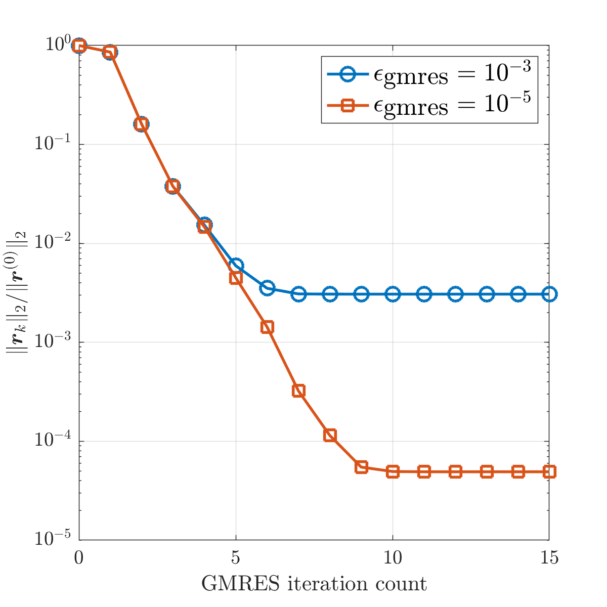 Figure 1
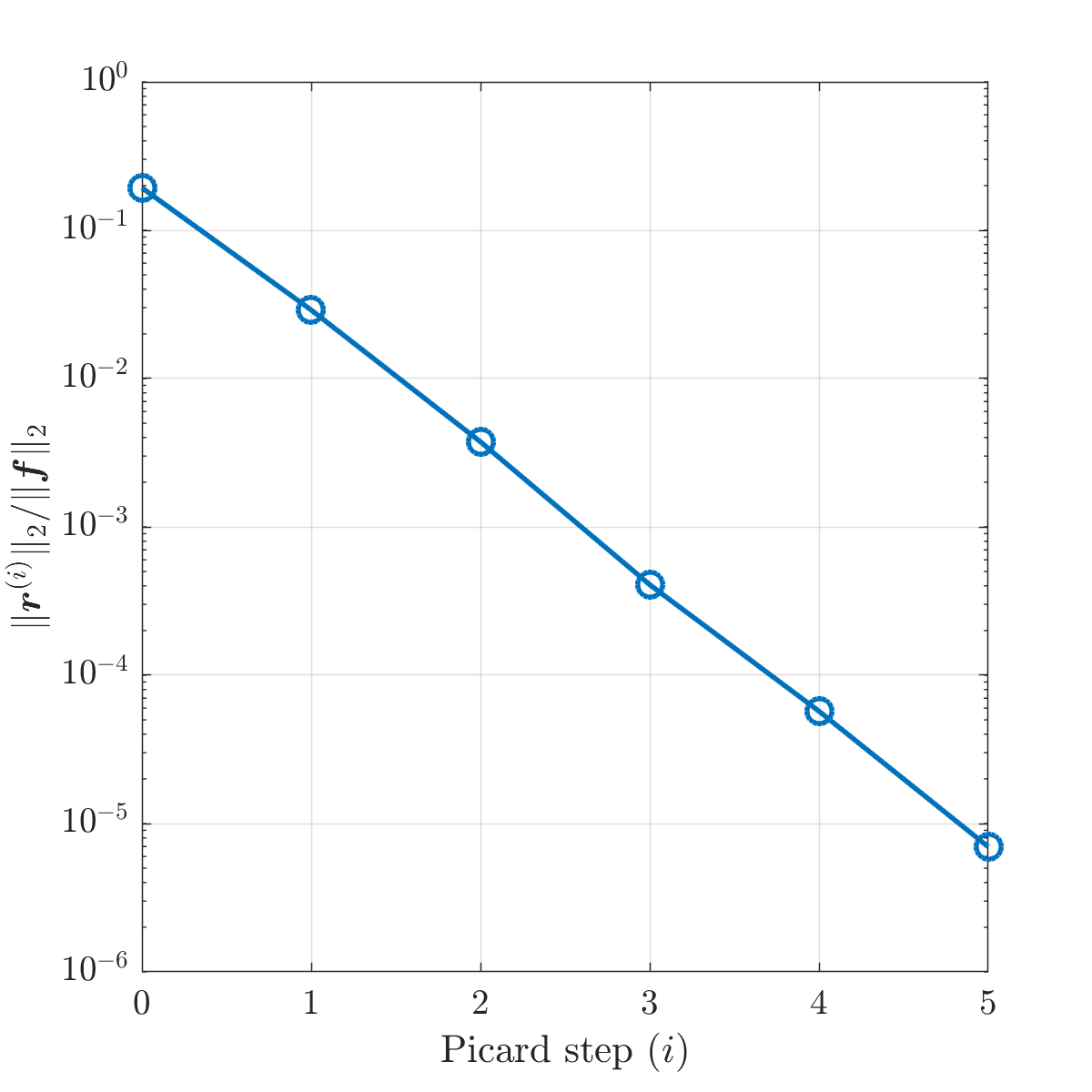 Figure 2
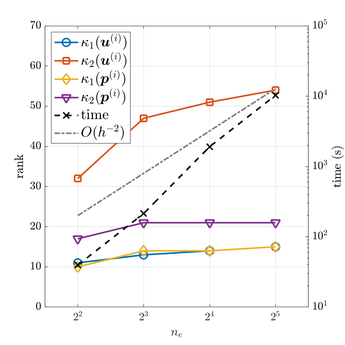 Figure 3
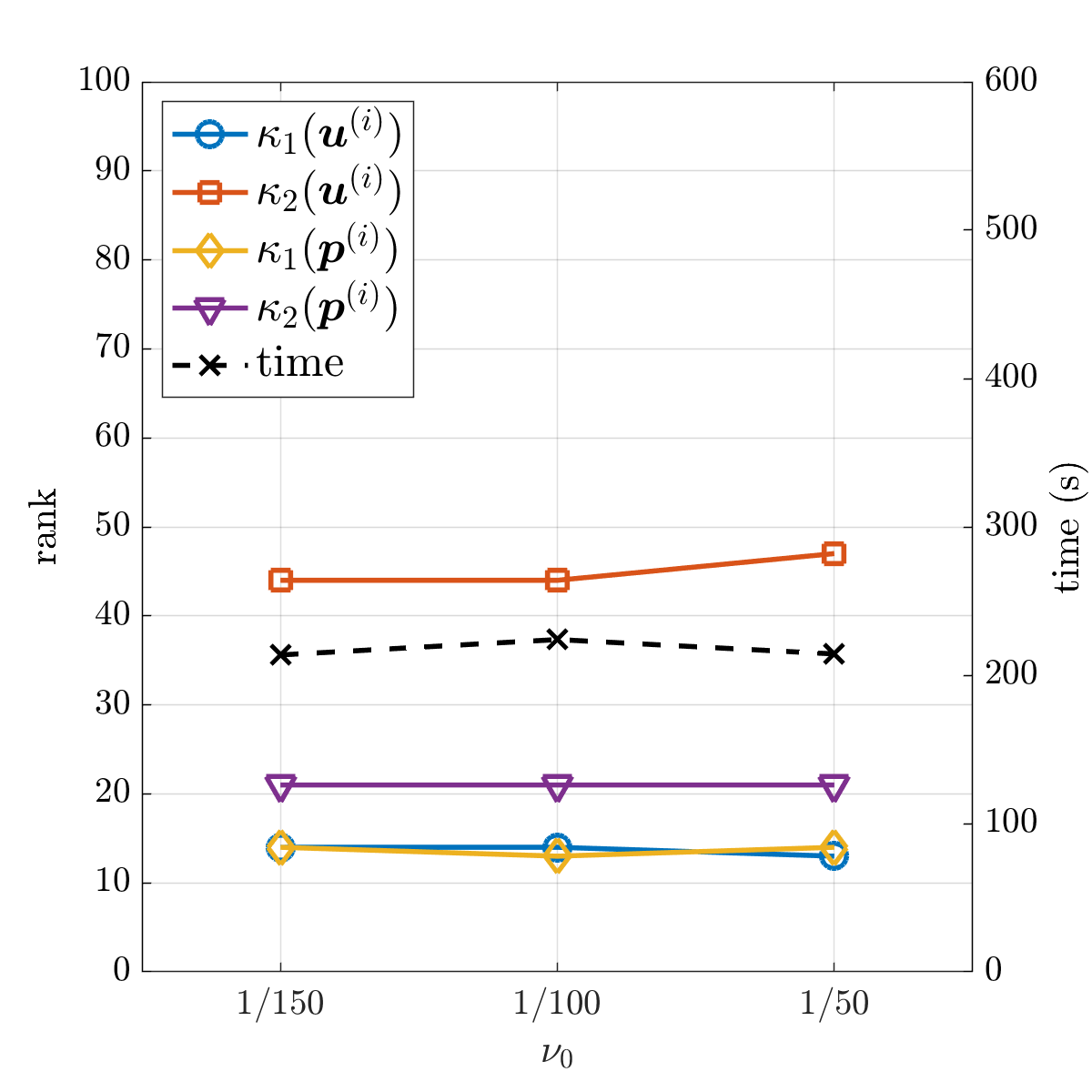 Figure 4
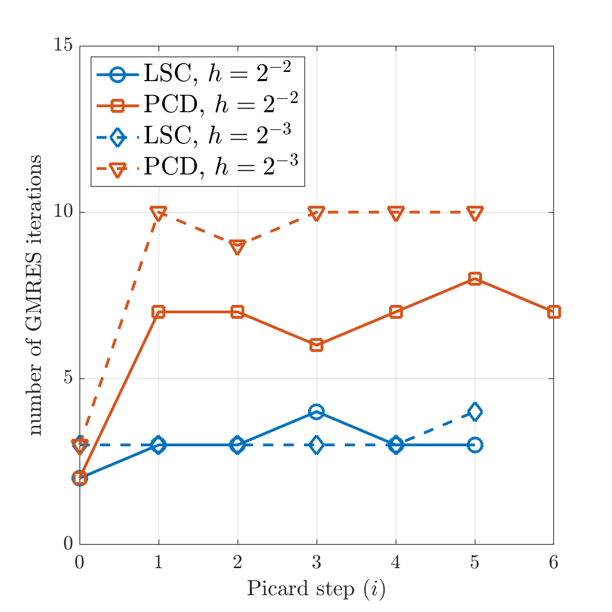 Figure 5
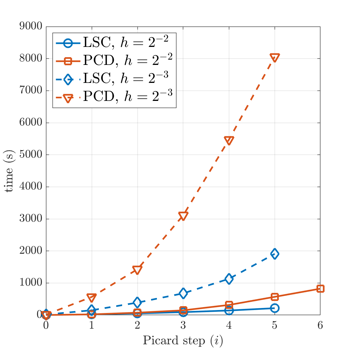 Figure 6
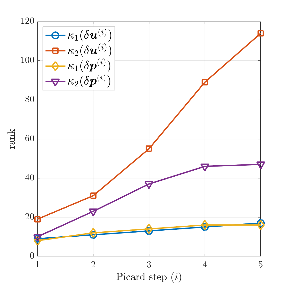 Figure 7
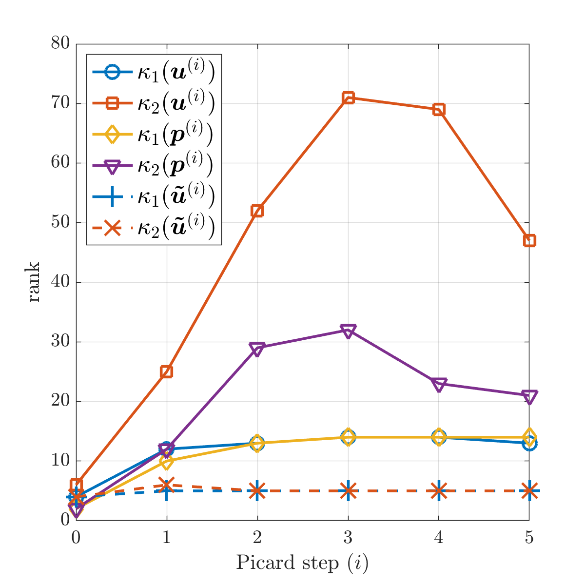 Figure 8
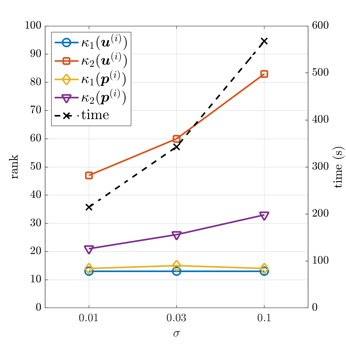 Figure 9
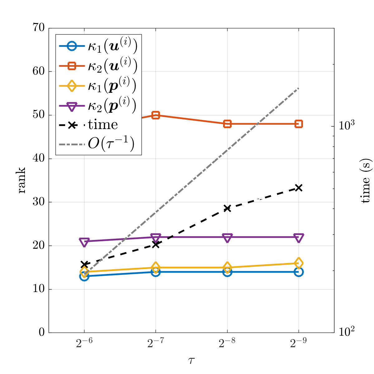 Figure 10
| 0.01 | 4.0 | 3 | 3 | 1.0 |
| GMRES stopping tolerance | |
|---|---|
| Picard stopping tolerance | |
| GMRES truncation tolerance | |
| Truncation tolerance for solutions | |
| Truncation tolerance for convection matrix |
| Number of Picard steps | 5 | 5 | 5 |
| Total number of GMRES iterations | 18 | 39 | 58 |
| Computational time (s) |
Peer Reviews
No public reviews on file for this paper yet. If you reviewed it on a platform where reviews are public (OpenReview, ICLR, NeurIPS, ICML), you can paste yours below so the community can read it here.
Videos
No videos yet. Explain this paper in a talk, walkthrough, or lecture? Add one.
\newsiamremark
remarkRemark
\headersLow-rank Solver for Stochastic Unsteady Navier–Stokes Problem H. C. Elman and T. Su
A Low-rank Solver for the Stochastic Unsteady Navier–Stokes Problem††thanks: This work was supported by the U.S. Department of Energy Office of Advanced Scientific Computing Research, Applied Mathematics program under award DE-SC0009301 and by the U.S. National Science Foundation under grant DMS1819115.
Howard C. Elman Department of Computer Science and Institute for Advanced Computer Studies, University of Maryland, College Park, MD 20742 (). [email protected]
Tengfei Su Applied Mathematics & Statistics, and Scientific Computation Program, University of Maryland, College Park, MD 20742 (). [email protected]
Abstract
We study a low-rank iterative solver for the unsteady Navier–Stokes equations for incompressible flows with a stochastic viscosity. The equations are discretized using the stochastic Galerkin method, and we consider an all-at-once formulation where the algebraic systems at all the time steps are collected and solved simultaneously. The problem is linearized with Picard’s method. To efficiently solve the linear systems at each step, we use low-rank tensor representations within the Krylov subspace method, which leads to significant reductions in storage requirements and computational costs. Combined with effective mean-based preconditioners and the idea of inexact solve, we show that only a small number of linear iterations are needed at each Picard step. The proposed algorithm is tested with a model of flow in a two-dimensional symmetric step domain with different settings to demonstrate the computational efficiency.
keywords:
time-dependent Navier–Stokes, stochastic Galerkin method, all-at-once system, low-rank tensor approximation
{AMS}
35R60, 60H35, 65F08, 65F10, 65N22
1 Introduction
Stochastic partial differential equations (PDEs) are widely used to model physical problems with uncertainty [16]. In this paper, we develop some new computational methods for solving the stochastic unsteady Navier–Stokes equations, using stochastic Galerkin methods [11] to address the stochastic nature of the problem and so-called all-at-once treatment of time integration.
For a time-dependent problem, the solutions at different time steps are usually computed in a sequential manner via time stepping. For example, a fully-implicit scheme with adaptive time step sizes was studied in [7, 14]. On the other hand, an all-at-once system can be formed by collecting the algebraic systems at all the discrete time steps into a single one, and the solutions are computed simultaneously. Such a formulation avoids the serial nature of time stepping, and allows parallelization in the time direction for accelerating the solution procedure [10, 18, 19]. A drawback, however, is that for large-size problems, the all-at-once system may require excessive storage. In this study, we address this issue by using a low-rank tensor representation of data within the solution methods.
We develop a low-rank iterative algorithm for solving the unsteady Navier–Stokes equations with an uncertain viscosity. The equations are linearized with Picard’s method. At each step of the nonlinear iteration, the stochastic Galerkin discretization gives rise to a large linear system, which is solved by a Krylov subspace method. Similar approaches have been used to study the steady-state problem [23, 27], where the authors also proposed effective preconditioners by taking advantage of the special structures of the linear systems. To reduce memory and computational costs, we compute low-rank approximations to the discrete solutions, which are represented as three-dimensional tensors in the all-at-once formulation. We refer to [12] for a review of low-rank tensor approximation techniques, and we will use the tensor train decomposition [21] in this work. The tensor train decomposition allows efficient basic operations on tensors. A truncation procedure is also available to compress low-rank tensors in the tensor train format to ones with smaller ranks.
Our goal is to use the low-rank tensors within Krylov subspace methods, in order to efficiently solve the large linear systems arising in each nonlinear step. The basic idea is to represent all the vector quantities that arise during the course of a Krylov subspace computation as low-rank tensors. With this strategy, much less memory is needed to store the data produced during the iteration. Moreover, the associated computations, such as matrix-vector products and vector additions, become much cheaper. The tensors are compressed in each iteration to maintain low ranks. This idea has been used for the conjugate gradient (CG) method and the generalized minimal residual (GMRES) method, with different low-rank tensor formats [1, 2, 5, 15]. In addition, the convergence of Krylov subspace methods can be greatly improved by an effective preconditioner. In conjunction with the savings achieved through low-rank tensor computations, we will derive preconditioners for the stochastic all-at-once formulation based on some state-of-the-art techniques used for deterministic problems, and we will demonstrate their performances in numerical experiments. We also explore the idea of inexact Picard methods where the linear systems are solved inexactly at each Picard step to further save computational work, and we show that with this strategy very small numbers of iterations are needed for the Krylov subspace method.
We note that a different type of approach, the alternating iterative methods [6, 13, 25], including the density matrix renormalization group (DMRG) algorithm and its variants, can be used for solving linear systems in the tensor train format. In these methods, each component of the low-rank solution tensor is approached directly and optimized by projecting to a small local problem. This approach avoids the rank growth in intermediate iterates typically encountered in a low-rank Krylov subspace method. However, these methods are developed for solving symmetric positive definite systems and require nontrivial effort to be adapted for a nonsymmetric Navier–Stokes problem.
The rest of the paper is organized as follows. In Section 2 we give a formal presentation of the problem. Discretization techniques that result in an all-at-once linear system at each Picard step are discussed in Section 3. In Section 4 we introduce the low-rank tensor approximation and propose a low-rank Krylov subspace iterative solver for the all-at-once systems. The preconditioners are derived in Section 5 and numerical results are given in Section 6.
2 Problem setting
Consider the unsteady Navier–Stokes equations for incompressible flows on a space-time domain ,
[TABLE]
where and stand for the velocity and pressure, respectively, is the viscosity, and is a two-dimensional spatial domain with boundary . The Dirichlet boundary consists of an inflow boundary and fixed walls, and Neumann boundary conditions are set for the outflow,
[TABLE]
We assume the Neumann boundary is not empty so that the pressure is uniquely determined. The function denotes a time-dependent inflow, typically growing from zero to a steady state, and it is set to zero at fixed walls. The initial conditions are zero everywhere for both and .
The uncertainty in the problem is introduced by a stochastic viscosity , which is modeled as a random field depending on a finite collection of random variables (or written as a vector ). Specifically, we consider a representation as a truncated Karhunen–Loève (KL, [17]) expansion,
[TABLE]
where is the mean viscosity, and are determined by the covariance function of . We assume that the random parameters are independent and that the viscosity satisfies almost surely for any . We refer to [23, 27] for different forms of the stochastic viscosity. The solutions and in Eq. 2.1 will also be random fields which depend on the space parameter , time , and the random variables .
3 Discrete problem
In this section, we derive a fully discrete problem for the stochastic unsteady Navier–Stokes equations Eq. 2.1. This involves a time discretization scheme and a stochastic Galerkin discretization for the physical and parameter spaces at each time step. The discretizations give rise to a nonlinear algebraic system. Instead of solving such a system at each time step, we collect the systems from all time steps to form an all-at-once system, where the discrete solutions at all the time steps are solved simultaneously. The discrete problem is then linearized with Picard’s method, and a large linear system is solved at each step of the nonlinear iteration.
3.1 Time discretization
For simplicity we use the backward Euler method for time discretization, which is first-order accurate but unconditionally stable and dissipative. The all-at-once formulation discussed later in section 3.3 requires predetermined time steps. Divide the interval into uniform steps with step size and initial time . Given the solution at time , we need to solve the following equations for and :
[TABLE]
After discretization (in physical space and parameter space) the implicit method requires solving an algebraic system at each time step. In the following we discuss how the system is assembled from the stochastic Galerkin discretization of Eq. 3.1.
3.2 Stochastic Galerkin method
At time step , the stochastic Galerkin method finds parametrized approximate velocity solutions and pressure solutions in finite-dimensional subspaces of and , where is the joint image of the random variables . The functional spaces are defined as follows,
[TABLE]
The expectations are taken with respect to the joint distribution of the random variables . In the following we use to denote the expected value. Let the finite-dimensional subspaces be , , and . Let and be the spaces of functions in with Dirichlet boundary conditions and imposed for the velocity field, respectively. Then for Eq. 3.1 the stochastic Galerkin formulation entails the computation of and , satisfying the weak form
[TABLE]
for any and . Here, denotes the inner product in . For the physical spaces, we use a div-stable Taylor–Hood discretization [8] on quadrilateral elements, with biquadratic basis functions for velocity, and bilinear basis functions for pressure. The stochastic basis functions are -dimensional orthonormal polynomials constructed from generalized polynomial chaos (gPC, [28]) satisfying . The stochastic Galerkin solutions are expressed as linear combinations of the basis functions,
[TABLE]
The coefficient vectors and similarly defined are computed from the nonlinear algebraic system
[TABLE]
where
[TABLE]
Here is the identity matrix, and denotes the Kronecker product of two matrices. The boldface matrices , , and are block-diagonal, with the scalar mass matrix , weighted stiffness matrix , and discrete convection operator as diagonal components, where
[TABLE]
for . Note the dependency on comes from the nonlinear convection term , with convection velocity . Let . The discrete divergence operator , with
[TABLE]
for and . The matrices and of Eq. 3.6 come from the stochastic basis functions and have entries
[TABLE]
for , where . These matrices are also sparse due to orthogonality of the basis functions [9]. The Dirichlet boundary conditions are incorporated in the right-hand side of Eq. 3.5.
3.3 All-at-once system
As discussed in the beginning of the section, we consider an all-at-once system where the discrete solutions at all the time steps are computed together. Let
[TABLE]
and let , , and be similarly defined. By collecting the algebraic systems Eq. 3.5 corresponding to all the time steps , we get the single system
[TABLE]
where is block diagonal with as the th diagonal block, , and with . Note that the zero initial conditions are incorporated in Eq. 3.5 for . The all-at-once system Eq. 3.11 is nonsymmetric and blockwise sparse. Each part of the system contains sums of Kronecker products of three matrices, i.e., in the form . In fact, from Eq. 3.6,
[TABLE]
We discuss later (see section 4.3) how the convection matrix can also be put in the Kronecker product form. It will be seen that this structure is useful for efficient matrix-vector product computations.
3.4 Picard’s method
We use Picard’s method to solve the nonlinear equation Eq. 3.11. Picard’s method is a fixed-point iteration. Let , be the approximate solutions at the th step. Each Picard step entails solving a large linear system
[TABLE]
Instead of Eq. 3.13, one can equivalently solve the corresponding residual equation for a correction of the solution. Let , . Then and satisfy
[TABLE]
where the nonlinear residual is
[TABLE]
Let denote the right-hand side of Eq. 3.11. The complete algorithm is summarized in Algorithm 3.1. The initial iterates , are obtained as the solution of a Stokes problem, for which in Eq. 3.13 the convection matrix is set to zero.
4 Low-rank approximation
In this section we discuss low-rank approximation techniques and how they can be used with iterative solvers. The computational cost of solving Eq. 3.14 at each Picard step is high due to the large problem size , especially when large numbers of spatial grid points or time steps are used to achieve high-resolution solution. We will address this using low-rank tensor approximations to the solution vectors and . We will develop efficient iterative solvers and preconditioners where the solution is approximated using a compressed data representation in order to greatly reduce memory requirements and computational effort. The idea is to represent the iterates in an approximate Krylov subspace method in a low-rank tensor format. The basic operations associated with the low-rank format are much cheaper, and as the Krylov subspace method converges it constructs a sequence of low-rank approximations to the solution of the system.
4.1 Tensor train decomposition
A tensor is a multidimensional array with entries , where , . The solution coefficients in Eq. 3.4 can be represented in the form of three-dimensional tensors (where ) and (), such that and . Equivalently, such tensors can be represented in vector format, where the vector version and are specified using the vectorization operation
[TABLE]
where , and in a similar manner. In an iterative solver for the system Eq. 3.14, any iterate can be equivalently represented as a three-dimensional tensor . In the sequel we use vector and tensor interchangebly. The tensor train decomposition [21] is a compressed low-rank representation to approximate a given tensor and efficiently perform tensor operations. Specifically, the tensor train format of is defined as
[TABLE]
where , , are the tensor train cores, and and are called the tensor train ranks. It is easy to see that if and is small, the memory cost to store is reduced from to .
The tensor train decomposition allows efficient basic operations on tensors. Most importantly, matrix-vector products can be computed much less expensively if the vector is in the tensor train format. For as in Eq. 4.2, the vector has an equivalent Kronecker product form [6]
[TABLE]
where in the right-hand side , , and are vectors of length , , and , respectively, obtained by fixing the indices and in , , and . Then for any matrix , such as the blocks in Eq. 3.14,
[TABLE]
The product is also in tensor train format with the same ranks as in (of the right-hand side of Eq. 4.2), and it only requires matrix-vector products for each component of . From left to right in the Kronecker products, the component matrices from Eq. 3.12 are sparse with numbers of nonzeros proportional to , , and , respectively, and the computational cost is thus reduced from to .
Other vector computations, including additions and inner products, are also inexpensive with the tensor train format. One thing to note is that the additions of two vectors in tensor train format will tend to increase the ranks. This can be easily seen from Eq. 4.2, since the addition of two low-rank tensors end up with more terms for the summation on the right-hand side. An important operation for the tensor train format is a truncation (or rounding) operation, used to reduce the ranks for tensors that are already in the tensor train format but have suboptimal high ranks. For a given tensor as in Eq. 4.2, the truncation operation with tolerance computes
[TABLE]
such that has smaller ranks than and satisfies the relative error
[TABLE]
(Note that .) The truncation operator is based on the TT-SVD algorithm [21], given in Algorithm 4.1, which is used to compute a low-rank tensor train approximation for a full tensor . In the algorithm, a sequence of singular value decompositions (SVDs) is computed for the so-called unfolding matrix , obtained by reshaping the entries of a tensor into a two-dimensional array. Terms corresponding to small singular values are dropped such that an error in the truncated SVD satisfies , (see line 4 of Algorithm 4.1). It was shown in [21] that the algorithm produces a tensor train that satisfies
[TABLE]
Thus, one can choose to make the relative error . Note the algorithm is costly since it requires SVDs on matrices . However, when the tensor is already in the tensor train format, the computation can be greatly simplified, and only SVDs on the much smaller tensor train cores are needed. In this case, the cost of the truncation operation is if and . We refer to [21] for more details. In the numerical experiments, we use TT-Toolbox [22] for tensor train computations.
4.2 Low-rank solver
The tensor train decomposition offers efficient tensor operations and we use it in iterative solvers to reduce the computational costs. The all-at-once system Eq. 3.14 to be solved at each step of Picard’s method is nonsymmetric. We use a right-preconditioned GMRES method to solve the system. The complete algorithm for solving is summarized in Algorithm 4.2. The preconditioner entails an inner iterative process and is not fixed for each GMRES iteration, and therefore a variant of the flexible GMRES method (see, e.g., [24]) is used. As discussed above, all the iterates in the algorithm are represented in the tensor train format for efficient computations, and a truncation operation with tolerance is used to compress the tensor train ranks so that they stay small relative to the problem size. It should be noted that since the quantities are truncated, the Arnoldi vectors do not form orthogonal basis for the Krylov subspace, and thus this is not a true GMRES computation. When the algorithm is used for solving Eq. 3.14, the truncation operator is applied to quantities associated with the two tensor trains and separately. In Section 5, we construct effective preconditioners for the system Eq. 3.14.
We also use the tensor train decomposition to construct a more efficient variant of Algorithm 3.1. In particular, the updated solutions and in line 5 are truncated, with a tolerance , so that
[TABLE]
Another truncation operation with is applied to compress the ranks of the nonlinear residual in line 7. We will use this truncated version of Algorithm 3.1 in numerical experiments; choices of the truncation tolerances will be specified in Section 6.
4.3 Convection matrix
We now show that in Eq. 3.12 if the velocity is in the tensor train format, the convection matrix can be represented as a sum of Kronecker products of matrices [3], which allows efficient matrix-vector product computations as in Eq. 4.4. Assume the coefficient tensor in Eq. 3.4 is approximated by a tensor train decomposition,
[TABLE]
Note that the entries of are linear in and
[TABLE]
Let . Then the th diagonal block of is
[TABLE]
The convection matrix can be expressed as
[TABLE]
Here is a vector obtained by fixing the index in , and is a diagonal matrix with on the diagonal. The result is a sum of Kronecker products of three smaller matrices. Such a representation can be constructed for any iterate in the tensor train format.
Given the number of terms in the summation in the right-hand side of Eq. 4.12, the matrix-vector product with will result in a dramatic tensor train rank increase, from to . Unless is very small, a tensor train with rank will require too much memory and also be expensive to work with. To overcome this difficulty, when solving the all-at-once system Eq. 3.14, we use a low-rank approximation of to construct . Specifically, let
[TABLE]
with some truncation tolerance . Since has smaller ranks than , the approximate convection matrix contains a smaller number of terms in Eq. 4.12, and thus the rank increase becomes less significant when computing matrix-vector products with it. In other words, the linear system solved at each Picard step becomes
[TABLE]
Note that the original is still used for computing the nonlinear residual in Picard’s method.
5 Preconditioning
In this section we discuss preconditioning techniques for the all-at-once system Eq. 3.14 so that the Krylov subspace methods converge in a small number of iterations. To simplify the notation, we use instead of , and the associated approximate solution at the th time step is
[TABLE]
with . In the following the dependence on in is omitted in most cases. We derive a preconditioner by extending ideas for more standard problems [8], starting with an “idealized” block triangular preconditioner
[TABLE]
With this choice of preconditioner, the Schur complement is , and the idealized preconditioned system derived from a block factorization
[TABLE]
has eigenvalues equal to 1 and Jordan blocks of order 2. (Here is an identity block.) Thus a right-preconditioned true GMRES method will converge in two iterations. However, the application of involves solving linear systems associated with and . These are too expensive for practical computation and to develop preconditioners we will construct inexpensive approximations to the linear solves. Specifically, we derive mean-based preconditioners that use results from the mean deterministic problem. Such preconditioners for the stochastic steady-state Navier–Stokes equations have been studied in [23]. We generalize the techniques for the all-at-once formulation of the unsteady equations.
5.1 Deterministic operator
We review the techniques used for approximating the Schur complement in the deterministic case [8]. The approximations are based on the fact that a commutator of the convection-diffusion operator with the divergence operator
[TABLE]
is small under certain assumptions about smoothness and boundary conditions. The subscript means the operators are defined on the pressure space. For a discrete convection-diffusion operator (which is part of the mean problem we discuss later), as defined in Eq. 3.7, an approximation to the Schur complement is identified from a discrete analogue of Eq. 5.4,
[TABLE]
where the subscript means the corresponding matrices constructed on the discrete pressure space. Equation 5.5 leads to an approximation to the Schur complement matrix,
[TABLE]
The pressure convection-diffusion (PCD) preconditioner is constructed by replacing the mass matrices with approximations containing only their diagonal entries (denoted by a subscript ) in Eq. 5.6,
[TABLE]
The least-squares commutator (LSC) preconditioner avoids the construction of matrices on the pressure space, with the approximation to ,
[TABLE]
(see [8, section 9.2] for a derivation). The LSC preconditioner is obtained by substituting in Eq. 5.6 and replacing the mass matrices with their diagonals,
[TABLE]
For both preconditioners, the only use of the matrices and is through matrix-vector products with them.
5.2 Approximations to
The Schur complement involves and is impractical to work with. For our stochastic unsteady problem, we consider mean-based preconditioners that use approximations to the Schur complement matrix
[TABLE]
where the “mean” matrix is block-diagonal with as the th diagonal block, and
[TABLE]
This corresponds to taking only the first term in the two summations on the right-hand side of Eq. 3.6. Since the gPC basis functions are orthonormal with and , it follows , and . The matrices and are constructed from the mean of and ,
[TABLE]
The matrix can be expressed as and this enables use of approximations associated with a deterministic problem. Now, similarly define on the pressure space, with
[TABLE]
Let and . Assuming the validity of Eq. 5.5 it is easy to check that
[TABLE]
On the other hand, let , so that satisfies
[TABLE]
Combining Eq. 5.14 and Eq. 5.15 gives an approximation to ,
[TABLE]
Then the mean-based PCD preconditioner is given as
[TABLE]
where and . Similarly from Eq. 5.8, it holds that
[TABLE]
Substituting in Eq. 5.17 and replacement of the mass matrices with their diagonals gives the mean-based LSC preconditioner
[TABLE]
The two mean-based preconditioners in Eqs. 5.17 and 5.19 have the same form as for the deterministic problem, except that there is an extra term or from the all-at-once formulation. Computations associated with the two approximations to the Schur complement are also inexpensive. For example, , and this only requires solving a system with a discrete Laplacian. Multiplications with the mean matrix are reduced to its components (see Eq. 4.4),
[TABLE]
The matrix is block-diagonal with and can be expressed as a sum of Kronecker products of matrices as discussed in section 4.3,
[TABLE]
5.3 System solve with
The application of the preconditioner in Eq. 5.2 also involves solving a linear system associated with the (1,1) block . For approximation, we replace it with the mean matrix , and solve a system of the form
[TABLE]
For such a system it is easy to compute matrix-vector products and we again use a low-rank GMRES method for solving the system. This inner GMRES solver is preconditioned with
[TABLE]
where is the average of over all time steps. For small time step , the contribution from the mass matrix, , becomes dominant and forms a good approximation to the coefficient matrix . The application of is also conveniently reduced to computations associated with smaller matrices. We note that Eq. 5.22 need not be solved accurately. In particular, with a stopping criterion , a relatively large stopping tolerance, e.g., , will suffice for the mean-based preconditioner to be effective.
Remark 5.1**.**
*For systems like Eq. 5.22, a block diagonal preconditioner () was studied in [20], where it was shown that preconditioned GMRES converges very slowly before a sharp drop in the residual occurs when the number of iterations reaches , which is equal to the number of diagonal blocks. In numerical experiments, we found that the preconditioner in Eq. 5.23 is more effective than a block diagonal one, for which performance deteriorates as becomes smaller. *
6 Numerical experiments
6.1 Benchmark problem
Consider a flow around a symmetric step where the spatial domain is a two-dimensional rectangular duct with a symmetric expansion (see Fig. 6.1). The Dirichlet inflow boundary conditions at , are deterministic and time-dependent, growing from zero to a steady parabolic profile,
[TABLE]
Neumann boundary conditions , are imposed at the outflow boundary , , and no-flow conditions at the fixed walls , ; , ; , . The initial conditions are zero everywhere for both and . The Taylor–Hood spatial discretization with biquadratic basis functions for the velocity space and bilinear basis functions for the pressure space is defined on a uniform grid of square elements with mesh size , and it is constructed using the IFISS software package [26].
The stochastic viscosity is represented as a truncated KL expansion
[TABLE]
The constants and represent the mean and the standard deviation of the stochastic field. We use an exponential covariance function , where is the correlation length. The pair is the th largest eigenvalue and the corresponding eigenfunction of , satisfying
[TABLE]
This can be computed with a standard finite element method. The random variables are assumed to be independent and each of them uniformly distributed on the interval , so they have zero means and unit variances. For the stochastic Galerkin method, the basis functions are -dimensional Legendre polynomials, with total degrees bounded by . Then the number of stochastic basis functions is . In the numerical experiments, unless otherwise stated, the parameter values associated with the discrete problem are chosen as in Table 6.1. This gives a problem with dimensions , , , , and . All computations are done in MATLAB 9.4.0 (R2018a) on a desktop with 64 GB memory.
6.2 Inexact Picard method
The main computational cost associated with Picard’s method is to solve an all-at-once system Eq. 3.14 at each step. In Section 4 we discussed how to construct low-rank approximate solutions in tensor train format with much cheaper computations. To further reduce the cost, we adopt the idea of inexact Picard method [4], where the linear systems are solved inexactly to save unnecessary computational work. Let Eq. 3.14 be denoted as , and define the residual norm for an approximate solution . It was shown in [4] that if the stopping criterion for the linear solve (line 2 of Algorithm 4.2) is given as
[TABLE]
then Picard’s method converges as long as . This is especially helpful for our low-rank GMRES method. The best accuracy that the low-rank GMRES method can achieve is related to the truncation tolerance used in the algorithm (see Fig. 6.2a). A relaxed stopping tolerance not only reduces the number of GMRES iterations, but it also allows use of larger truncation tolerances for tensor rank compressions, resulting in smaller ranks for the iterates and more efficient computations in the iterative solver. In the numerical tests, we set and . The same tolerances are used for solving the linear system Eq. 5.22 required for the preconditioning operation. For the initial , , the Stokes problem is solved to satisfy where is the right-hand side of Eq. 3.13.
6.3 Numerical results
In the following, we examine the performance of the proposed low-rank algorithm in different settings. The choices of stopping and truncation tolerances are summarized in Table 6.2. In Algorithm 3.1, the stopping criterion for Picard’s method is
[TABLE]
We set . A small truncation tolerance is used to produce low-rank approximate solutions and in Eq. 4.8. It is shown in Fig. 6.2b that, like the exact method, the inexact Picard method still exhibits a linear convergence rate. It takes 5 Picard steps to reach the required accuracy. Figure 6.3 shows the tensor train ranks and of the iterates at each Picard step. As the Picard iteration converges, the right-hand side of Eq. 6.4 becomes smaller, and the corrections and computed from the low-rank GMRES method have increasing ranks. On the other hand, for the approximate solutions and , their ranks drop to smaller values in the latter steps of the iteration. With a more stringent , a smaller is required and the approximate solutions have slightly higher ranks than those shown in Fig. 6.3b. Also shown in Fig. 6.3b are the tensor train ranks of for constructing the approximate convection matrices using Eq. 4.13. They have much smaller values than the ranks of .
We demonstrate the savings obtained from the inexact solves. Table 6.3 shows the performance of Picard’s method if different stopping tolerances are used in Eq. 6.4. With a larger , the number of Picard steps does not increase, while the total number of GMRES iterations and the associated computational costs are greatly reduced.
We compare the two mean-based preconditioners discussed in Section 5. Figure 6.4 shows the number of GMRES iterations required at each Picard step, and the associated computational costs when the two preconditioners are used. For two different mesh sizes, the PCD preconditioner results in larger numbers of GMRES iterations, and thus higher computational times, than the LSC preconditioner. It should also be noted that for both preconditioners, only a small number of GMRES iterations is needed for solving the linear system at each Picard step. This is partially due to the large stopping tolerance used in Eq. 6.4. The LSC preconditioner will be used for the numerical tests below.
In the following, we test the algorithm with several variants of the benchmark problem determined by various values of parameters associated with it. Figure 6.5a shows the solution ranks and computational times for three different values of . When is smaller, the standard deviation is smaller, the discrete solution can be approximated by a tensor train with smaller ranks, and it is also less expensive to solve the nonlinear problem. On the other hand, even for , the low-rank solution takes much less storage than a full tensor. For example, the ranks of the approximate solution are , . The ratio of storage requirements between such a tensor train and a full tensor is
[TABLE]
The same quantities are plotted in Fig. 6.5b for different values of the mean viscosity . The ranks and computational times are not significantly affected by .
Finally, the algorithm is applied to solve discrete problems with various mesh sizes or time step sizes . It can be seen from Fig. 6.6a that there is only a slight increase in the solution ranks as the spatial mesh is refined. It is also shown in Fig. 6.6a that the computational time increases with an asymptotic rate (note that a logarithmic scale is used in the figure). In other words, as the spatial mesh is refined, no extra computational burden is introduced except for the increased problem size. For different time step sizes , the computational time increases much more slowly than (see Fig. 6.6b). This is due to the fact that in , the matrices obtained from time discretization are very simple (e.g., and ), and thus an increase in does not make a significant impact on the computational costs.
7 Conclusions
In this paper, we developed and studied efficient low-rank iterative methods for solving the time-dependent Navier–Stokes equations with a random viscosity. We considered an all-at-once formulation where the discrete solutions at all the time steps are solved together in a single system. To address the high storage and computational costs of this strategy, we used low-rank tensor approximations in a Newton–Krylov type algorithm. For the all-at-once system, we proposed two mean-based preconditioners using results from the deterministic problem. The computational costs were further reduced with inexact Picard method and approximate convection matrices. It was shown in the numerical experiments that the low-rank method is able to solve the nonlinear problem efficiently and the discrete solutions have small tensor ranks.
The reference list from the paper itself. Each links out to its DOI / PubMed record.
- 1[1] R. Andreev and C. Tobler , Multilevel preconditioning and low-rank tensor iteration for space-time simultaneous discretizations of parabolic PD Es , Numerical Linear Algebra with Applications, 22 (2015), pp. 317–337.
- 2[2] J. Ballani and L. Grasedyck , A projection method to solve linear systems in tensor format , Numerical Linear Algebra with Applications, 20 (2013), pp. 27–43.
- 3[3] P. Benner, S. Dolgov, A. Onwunta, and M. Stoll , Solving optimal control problems governed by random Navier–Stokes equations using low-rank methods , Mar. 2017, https://arxiv.org/abs/1703.06097 .
- 4[4] P. Birken , Termination criteria for inexact fixed-point schemes , Numerical Linear Algebra with Applications, 22 (2015), pp. 702–716.
- 5[5] S. V. Dolgov , TT-GMRES: solution to a linear system in the structured tensor format , Russian Journal of Numerical Analysis and Mathematical Modelling, 28 (2013), pp. 149–172.
- 6[6] S. V. Dolgov and D. V. Savostyanov , Alternating minimal energy methods for linear systems in higher dimensions , SIAM Journal on Scientific Computing, 36 (2014), pp. A 2248–A 2271.
- 7[7] H. Elman, M. Mihajlović, and D. Silvester , Fast iterative solvers for buoyancy driven flow problems , Journal of Computational Physics, 230 (2011), pp. 3900–3914.
- 8[8] H. C. Elman, D. J. Silvester, and A. J. Wathen , Finite Elements and Fast Iterative Solvers: With Applications in Incompressible Fluid Dynamics , Oxford University Press, UK, second ed., 2014.