Meta-learning Pseudo-differential Operators with Deep Neural Networks
Jordi Feliu-Faba, Yuwei Fan, Lexing Ying

TL;DR
This paper presents a meta-learning method using deep neural networks to efficiently approximate parameterized pseudo-differential operators, enabling accurate solutions for complex PDEs with limited computations.
Contribution
It introduces a novel meta-learning framework that combines wavelet transforms and neural networks to approximate pseudo-differential operators from minimal data.
Findings
Efficient approximation of Green's functions for elliptic PDEs.
Accurate modeling of radiative transfer equations.
Reduced computational cost for operator evaluation.
Abstract
This paper introduces a meta-learning approach for parameterized pseudo-differential operators with deep neural networks. With the help of the nonstandard wavelet form, the pseudo-differential operators can be approximated in a compressed form with a collection of vectors. The nonlinear map from the parameter to this collection of vectors and the wavelet transform are learned together from a small number of matrix-vector multiplications of the pseudo-differential operator. Numerical results for Green's functions of elliptic partial differential equations and the radiative transfer equations demonstrate the efficiency and accuracy of the proposed approach.
Click any figure to enlarge with its caption.
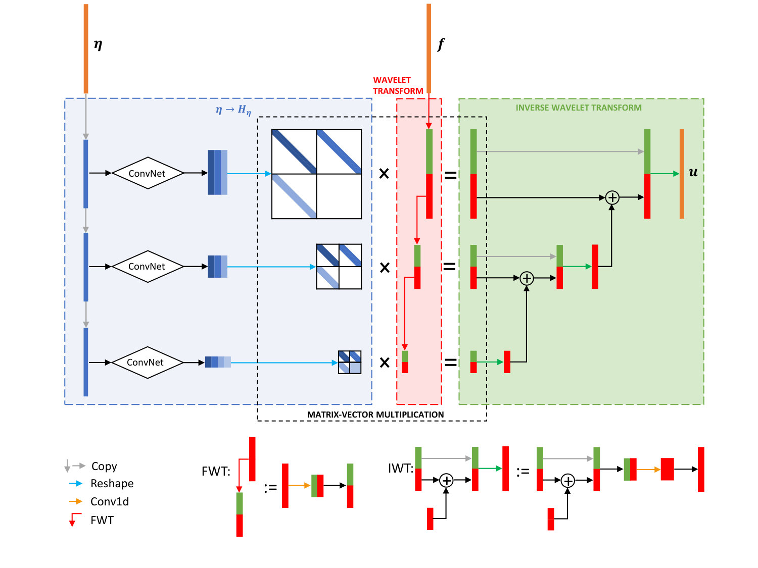 Figure 1
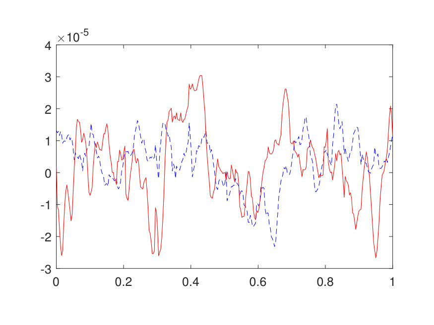 Figure 2
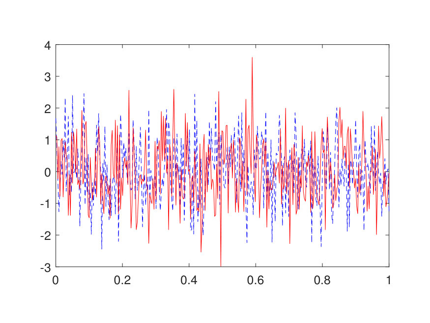 Figure 3
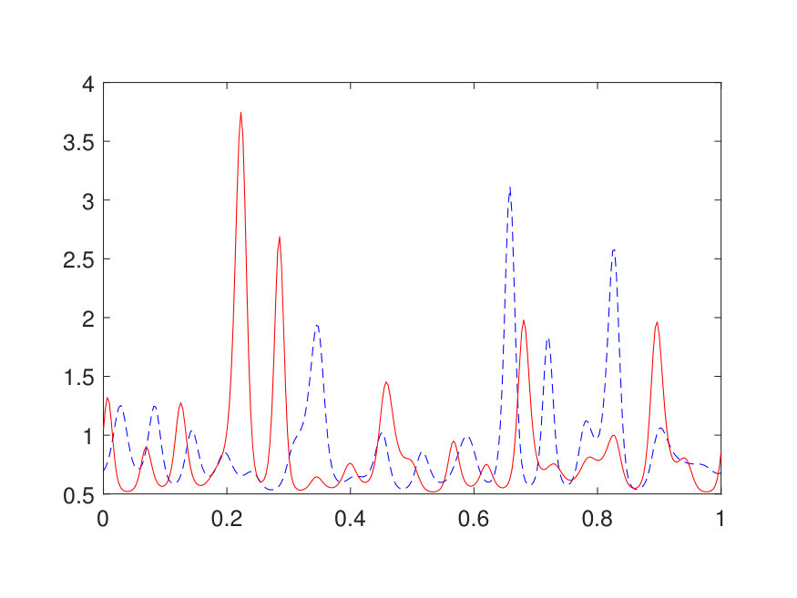 Figure 4
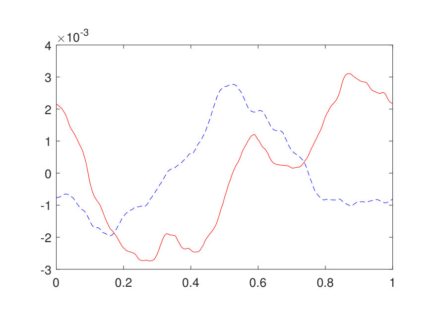 Figure 5
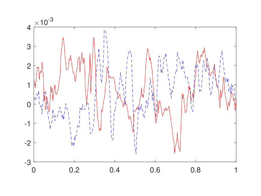 Figure 6
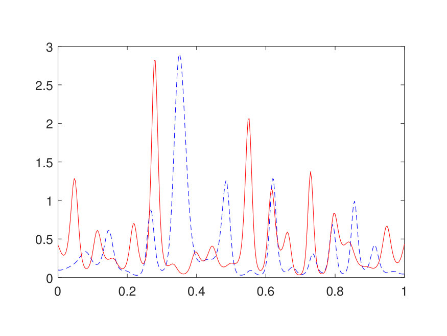 Figure 7
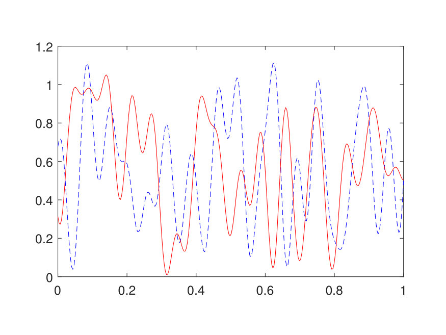 Figure 8
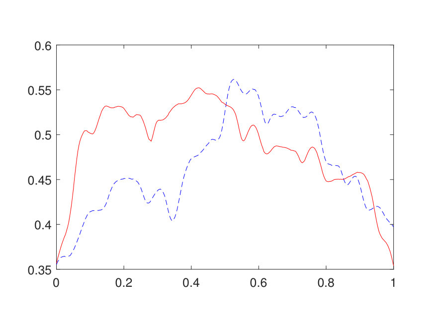 Figure 9
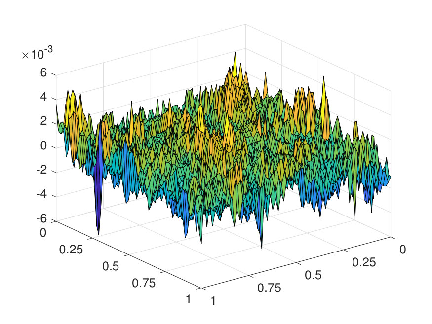 Figure 10
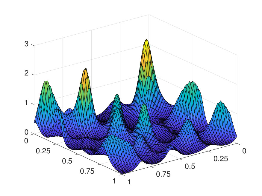 Figure 11
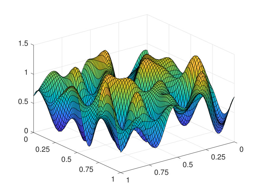 Figure 12
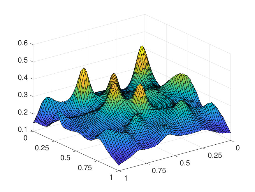 Figure 13
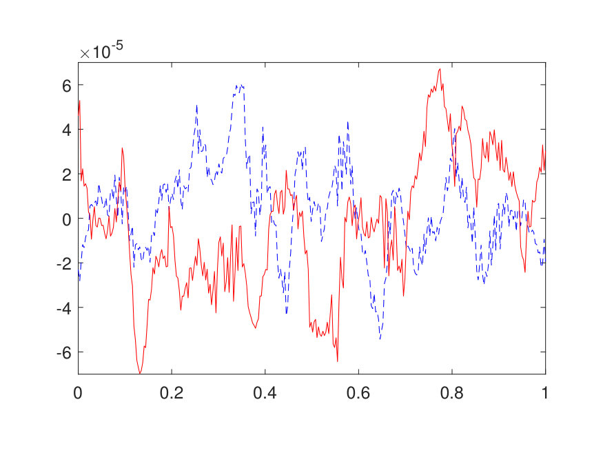 Figure 14
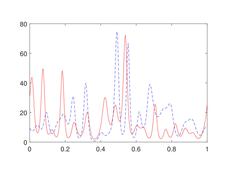 Figure 15
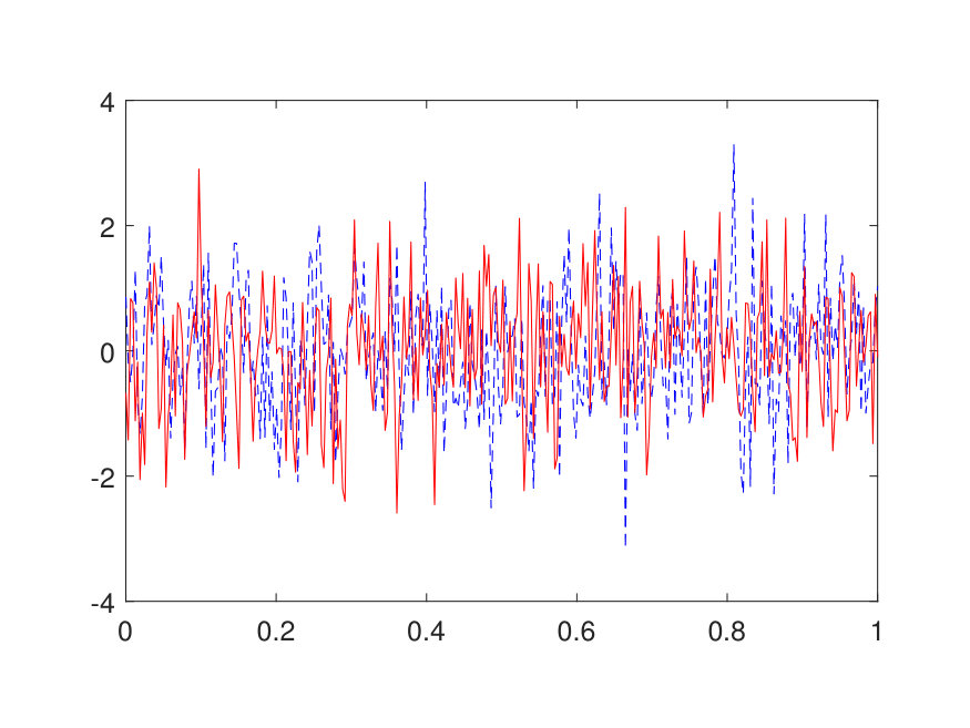 Figure 16
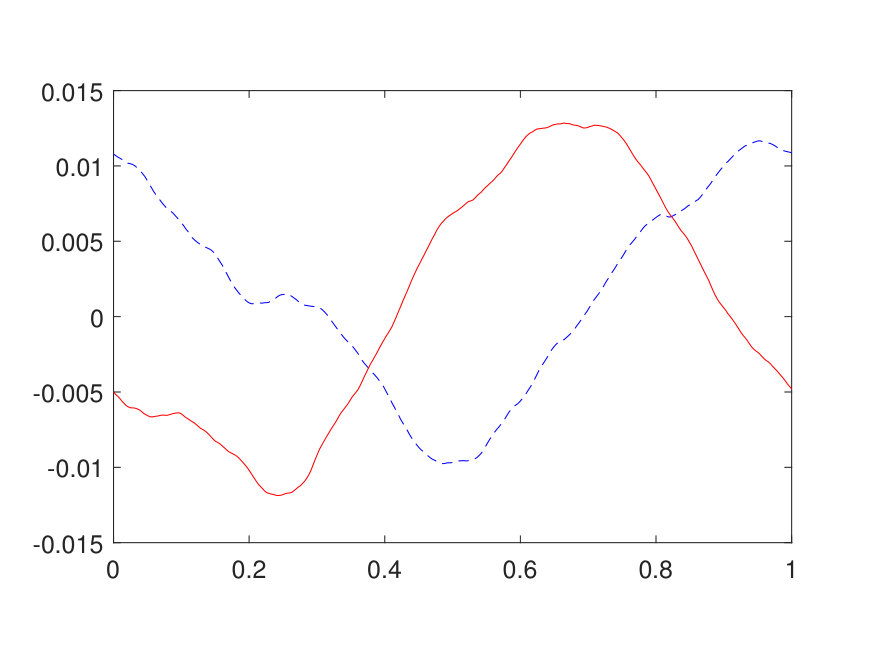 Figure 17
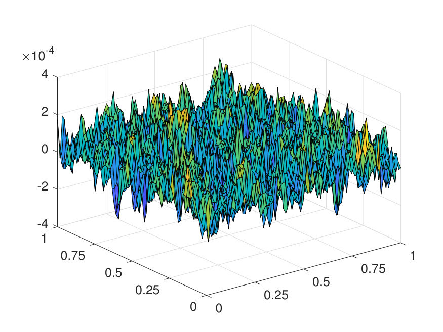 Figure 18
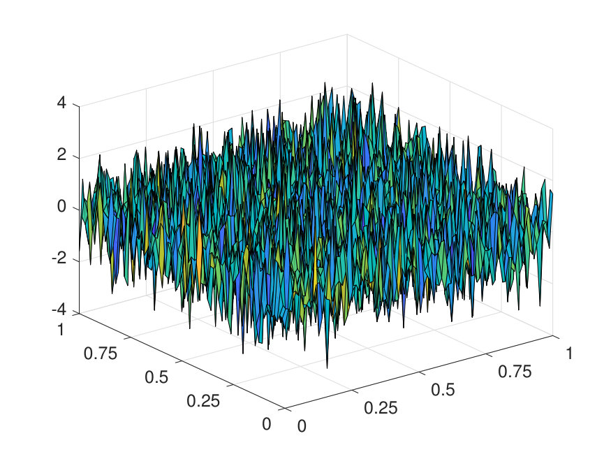 Figure 19
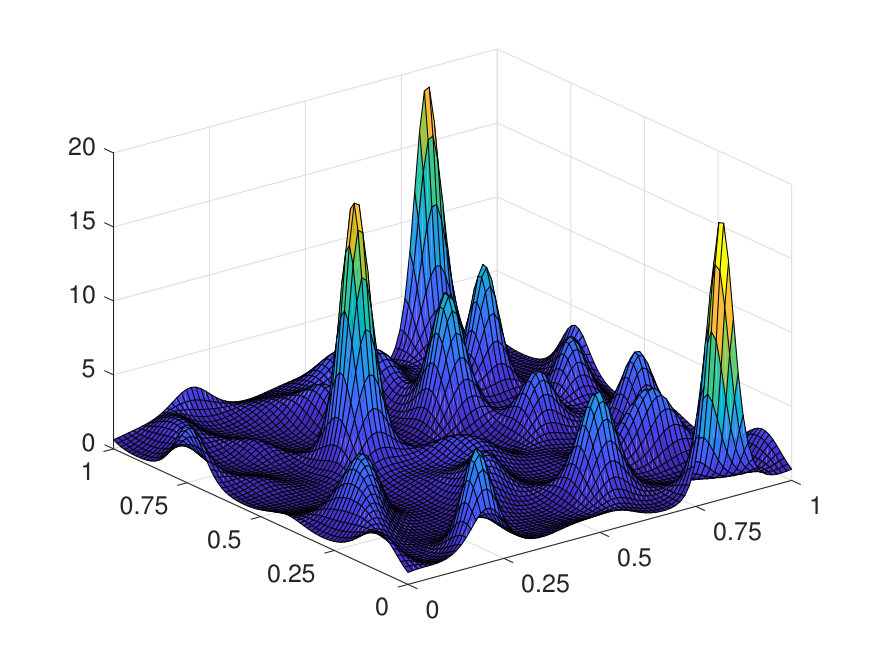 Figure 20
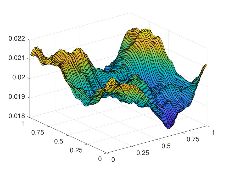 Figure 21
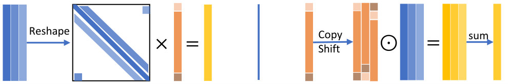 Figure 22
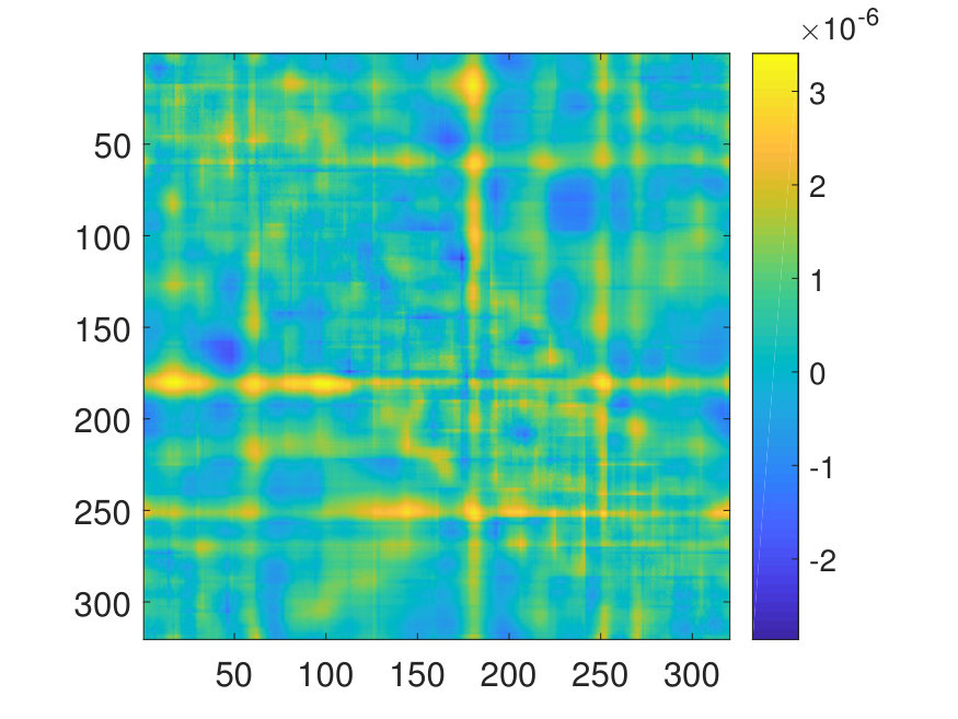 Figure 23
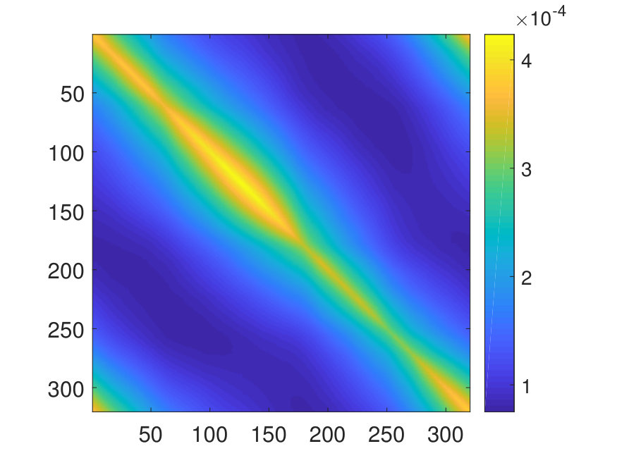 Figure 24
 Figure 25
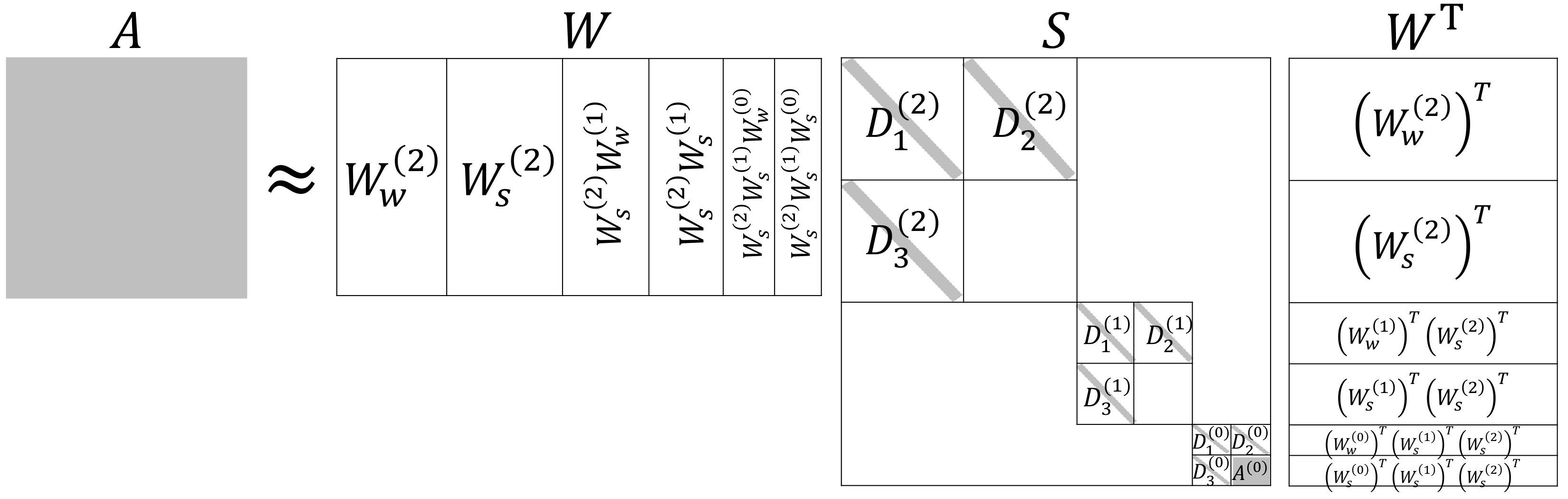 Figure 26
| 5 | 5 | 30201 | 4.43e-3 | 4.74e-3 | 2.49e-3 |
| 5 | 7 | 38061 | 4.83e-3 | 5.18e-3 | 4.28e-3 |
| 7 | 5 | 58717 | 4.09e-3 | 4.35e-3 | 3.28e-3 |
| 7 | 7 | 74089 | 4.11e-3 | 4.42e-3 | 2.18e-3 |
| 11 | 5 | 930447 | 2.21e-2 | 2.18e-2 | 4.17e-3 |
|---|---|---|---|---|---|
| 15 | 5 | 1226071 | 2.12e-2 | 2.10e-2 | 2.04e-3 |
| 7 | 5 | 58717 | 7.27e-3 | 7.76e-3 |
| 7 | 7 | 74089 | 7.46e-3 | 8.29e-3 |
| 9 | 5 | 96625 | 6.05e-3 | 6.88e-3 |
| 9 | 7 | 122005 | 6.83e-3 | 8.21e-3 |
| 5 | 5 | 34131 | 2.48e-3 | 2.93e-3 |
| 5 | 7 | 41991 | 2.46e-3 | 3.01e-3 |
| 7 | 5 | 66403 | 1.92e-3 | 2.45e-3 |
| 7 | 7 | 81775 | 2.05e-3 | 2.36e-3 |
| 11 | 5 | 1287903 | 4.39e-3 | 4.39e-3 |
| 15 | 5 | 1663831 | 3.55e-3 | 3.55e-3 |
Peer Reviews
No public reviews on file for this paper yet. If you reviewed it on a platform where reviews are public (OpenReview, ICLR, NeurIPS, ICML), you can paste yours below so the community can read it here.
Videos
No videos yet. Explain this paper in a talk, walkthrough, or lecture? Add one.
Meta-learning Pseudo-differential Operators
with Deep Neural Networks
Jordi Feliu-Fabà , Yuwei Fan , Lexing Ying ICME, Stanford University, Stanford, CA 94305. Email: [email protected] of Mathematics, Stanford University, Stanford, CA 94305. Email: [email protected] of Mathematics and ICME, Stanford University, Stanford, CA 94305. Email: [email protected]
Abstract
This paper introduces a meta-learning approach for parameterized pseudo-differential operators with deep neural networks. With the help of the nonstandard wavelet form, the pseudo-differential operators can be approximated in a compressed form with a collection of vectors. The nonlinear map from the parameter to this collection of vectors and the wavelet transform are learned together from a small number of matrix-vector multiplications of the pseudo-differential operator. Numerical results for Green’s functions of elliptic partial differential equations and the radiative transfer equations demonstrate the efficiency and accuracy of the proposed approach.
Keywords: Deep neural networks; Convolutional neural networks; Nonstandard wavelet form; Meta-learning; Green’s functions; Radiative transfer equation.
1 Introduction
Many physical models for scientific and engineering applications can be written in a general form
[TABLE]
for a domain with appropriate boundary conditions, where is often a partial differential or integral operator parameterized by a parameter function . Solving for for a given amounts to representing the inverse operator (sometimes also known as the Green’s function) either explicitly or implicitly via an efficient algorithm. Representing , even if implicitly, can be computationally challenging, especially for multidimensional problems. The past few decades have witnessed steady progresses in developing efficient algorithms for this.
Problem statement.
This paper is concerned with a more ambitious task: representing the nonlinear map from to
[TABLE]
when the operator is a pseudo-differential operator (PDO) [60]. Although and can be linear operators, this map from to is highly nonlinear.
Background.
In the recent years, deep learning has become the most versatile and effective tool in artificial intelligence and machine learning, witnessed by impressive achievements in computer vision [36, 61, 28], speech and natural language processing [29, 56, 51, 57, 11], drug discovery [43] or game playing [54, 15, 58]. Recent reviews on deep learning and its impacts on other fields can be found in for example [38, 53]. At the center of deep learning, the model of deep neural networks (NNs) provides a flexible framework for approximating high-dimensional functions, while allowing for efficient training and good generalization properties in practice [42, 47].
More recently, several groups have started applying NNs to partial differential equations (PDEs) and integral equations (IEs) arising from physical systems. In one direction, the NN model has been used to approximate solutions of high-dimensional PDEs [37, 55, 14, 49, 4, 6, 13, 25, 32, 41]. In a somewhat orthogonal direction, the NNs have been utilized to approximate the high-dimensional parameter-to-solution of various PDEs and IEs [31, 26, 18, 17, 19, 33, 25, 2, 39, 20].
Another topic from machine learning that is particularly relevant to this work is meta-learning or learning-to-learn [52, 3, 27, 21, 59]. A meta-learning system learns to produce learning models for new tasks and scenarios from their metadata with zero or minimum amount of new data, by leveraging the common structure among different tasks. Due to the low requirements on new data points, meta-learning has gained a lot of attention in recent years in applications such as vision and reinforcement learning.
Main idea.
Following these recent advances in applying NNs to physical models, this paper takes a deep learning approach for representing the map in Eq. 1.2. The most straightforward solution would be to take a supervised learning approach, i.e., trying to learn the map from a large set of training data . However, since it is often difficult or even impossible to compute and store due to the enormous discretization size, this straightforward supervised learning approach is not practical for Eq. 1.2.
Without explicit access to , we take a meta-learning approach, i.e., learning to produce, for each new , an NN approximation to . To do this, we are faced with two key difficulties.
- •
How should we represent the output for an arbitrary input ?
- •
How should we represent the training data?
To address the first question, should be represented in a compressed form. For pseudo-differential operators, several compressed representations exist, including hierarchical matrices [22, 23, 24], discrete symbol calculus [10], etc. In this paper, we choose to represent with the nonstandard wavelet form introduced in [5]. The main advantage of the nonstandard wavelet form is that the nonzero entries of this compressed representation are simply organized into a small number of vectors. More precisely,
[TABLE]
where is a redundant form of a wavelet transform, stands for the collection of vectors that contain the nonzero entries of the compressed form, and is a certain operator that generates a sparse matrix from the vector collection . Compared to [5], a key difference is that the current approach allows for to be fine-tuned for the map .
To address the second question, instead of explicitly representing , the training data consists of samples of the form
[TABLE]
where . For a fixed , such data can be obtained by solving the equation for each , possibly with a fast algorithm.
Putting these two pieces together, the meta-learning approach of this paper learns two following key objects from the training data of form :
- •
a map from to the vector collection ,
- •
the -dependent wavelet transform .
Once trained, for a given test input the architecture calculates and returns a linear NN that implements .
Organization.
The rest of this paper is organized as follows. Section 2 briefly reviews the nonstandard wavelet form, used for representing . In Section 3, the NN architecture of the meta-learning approach is discussed in detail. Section 4 applies the proposed NN to the Green’s function of elliptic PDEs, in both the Schrödinger form and the divergence form. The application to the radiative transfer equation is presented in Section 5.
2 Nonstandard wavelet form
This section summarizes the nonstandard wavelet form proposed in [5]. To make things concrete, compactly supported orthonormal Daubechies wavelets [8] are used as the basis functions as an example.
2.1 Wavelet transform
In the one-dimensional multiresolution analysis, one starts by defining a scaling function that generates, through dyadic translations and dilations, a family of functions
[TABLE]
For each scale , the functions form a Ritz basis for a space , which satisfies a nested relationship . This nested property of implies the following dilation relation of the scaling function
[TABLE]
For the Daubechies’ wavelets [8], the scaling function has a compact support for a given positive integer and therefore the coefficients are only nonzero for . The scaling function also satisfies the orthonormal condition
[TABLE]
which leads to an orthonormal condition for the coefficients
[TABLE]
Given the scaling function , another important component of the multiresolution analysis is the wavelet function , defined by
[TABLE]
where for . A simple calculation shows that the support of is and is nonzero only for , based on the support of the and the nonzero entries pattern of . The Daubechies wavelets are then defined as
[TABLE]
For a function , its scaling and wavelet coefficients and are defined as the inner product with the scaling functions and the wavelets
[TABLE]
Using the recursive relationships of the scaling function Eq. 2.2 and the wavelet function Eq. 2.5, one obtains a recursive relationship of the scaling and wavelet coefficients
[TABLE]
By defining and , Eq. 2.8 can be written in a matrix form
[TABLE]
where the operators and are banded with a bandwidth due to the support of and . By introducing the orthogonal operator , Eq. 2.9 can be rewritten as
[TABLE]
The procedure for computing the wavelet and scaling coefficients can be illustrated in the following diagram
[TABLE]
The discussion until now is concerned with the wavelets on . It is straightforward to extend it the functions defined on a finite domain with periodic boundary condition. If the function is periodic on a finite domain, for instance, , then the only modification is that all the shifts and scaling in the variable are done modulus the integer. When working with periodic functions, the procedure in Eq. 2.11 usually stops at a coarse level before the wavelet and scaling functions start to overlap itself.
[TABLE]
2.2 Nonstandard wavelet form for integral operator
Let be an integral operator with kernel , applied to periodic functions defined on , i.e.,
[TABLE]
Denote by the Galerkin projection of to the space , for a sufficiently deep level , i.e.
[TABLE]
The nonstandard form described in [5] is a remarkably efficient way to compress the matrix .
The main step for the nonstandard form is to treat as an image and use the 2D multiresolution analysis
[TABLE]
for , and . For convenience, these coefficients are organized into the matrix form as
[TABLE]
In this setting, a similar recursive relation to Eq. 2.10 can be obtained
[TABLE]
If is a Calderon-Zygmund operator, the entries of the matrices with decay rapidly away from the diagonal. For a prescribed relative accuracy , each matrix can be approximated by a band matrix by truncating at a band of width . Since the bandwidth is independent of the specific choices of , , or the mesh size , the nonstandard form of stores only nonzero entries. The readers are referred to [5] for more details. With a slight abuse of notation, the matrices are assumed to be pre-truncated in what follows.
One can assemble all the matrices and together, by defining the matrix in a recursive way as
[TABLE]
The matrix is the nonstandard form of the matrix satisfying
[TABLE]
Here is the extended wavelet transform matrix, defined in the recursive form as
[TABLE]
Figure 1 illustrates the matrices and along with the formulation Eq. 2.18.
To clarify the notations, we denote by and the transform matrices defined in Eq. 2.9 for the scaling and wavelet parts on level , respectively. is the wavelet transform matrix at the level .
2.3 Matrix-vector multiplication in the nonstandard form
With a Galerkin discretization of Eq. 2.13 at level , the matrix-vector multiplication takes the form
[TABLE]
The nonstandard form allows for accelerating the evaluation of Eq. 2.20. Using the nonstandard form obtained above, the matrix-vector multiplication
[TABLE]
can be split into four steps:
: generate the nonstandard form from the matrix or the kernel ; 2. 2.
: apply (forward) wavelet transform on to get ; 3. 3.
: evaluate the matrix-vector multiplication in the nonstandard form; 4. 4.
: apply inverse wavelet transform on to obtain .
The first step is computed using Eq. 2.16 if the matrix is given. The second step follows Eq. 2.10. The third step can be written as
[TABLE]
where for and . The fourth step is essentially an inverse wavelet transform, implemented as
[TABLE]
A step-by-step description of these four steps are summarized in Algorithm 1.
2.4 The multidimensional case
The matrix-vector multiplication in the nonstandard form can be easily extended to the multidimensional case with the help of multidimensional orthogonal wavelets (see [44] for more details). For instance, in the two-dimensional setting, one defines at each scale three different types of wavelets of the form
[TABLE]
with . Using these three types of wavelets, the transform matrix at each scale used in Eq. 2.10 is redefined to be . The 2D analog of Eq. 2.10 contains three types of wavelet coefficients
[TABLE]
Similarly, the recursive relation Eq. 2.16 can be extended as well
[TABLE]
where , are all sparse matrices with only non-negligible entries in each. The matrix-vector multiplication follows the steps of Algorithm 1, with these necessary changes.
3 Meta-learning approach
The plan is to apply the nonstandard form to the operator in Eq. 1.2
[TABLE]
With a slight abuse of notations, the same letters are used to denote the discretizations. The discrete version of Eq. 3.1 takes the form
[TABLE]
with . The main goal of this paper is to construct a neural network to learn the map .
Following Eq. 2.18 and applying the wavelet transform to the matrix leads to
[TABLE]
where is the extended wavelet transform matrix, independent of the parameter . Since each block of matrix is a band matrix, the nonzero entries of each block can be represented by a set of vectors. Let us define , of size , to be the collection of these vectors of at level , with dependent on the bandwidth and . By introducing the collection of vectors , is uniquely determined by , i.e.,
[TABLE]
for a fixed embedding operator determined by the sparsity pattern of .
Given a set of training samples of the form
[TABLE]
where can be obtained by solving with right hand side , the meta-learning approach first learns both the map and the wavelet transform matrix . Once they are ready, given any new , can be approximated by evaluating the map and representing (3.3) in an NN form.
3.1 Neural network architecture
Using the factorization of in Eq. 3.3, one can factorize as
[TABLE]
Similar to the matrix-vector multiplication in Section 2.3 of the nonstandard form, we propose a neural network for meta-learning Eq. 3.5 with four modules:
: a module learns the map and then generates the banded sparse matrix from (denoted as ); 2. 2.
: a module applies the forward wavelet transform to to generate ; 3. 3.
: a module evaluates the matrix-vector multiplication in the nonstandard form; 4. 4.
: a module applies the inverse wavelet transform on to generate .
Instead of computing from the full operator as described in Section 2.3. the first module forms directly from the parameter using a deep NN. This module can be split into two steps: (1) carrying out the map for each scale ; (2) constructing the nonstandard form from . The NN architecture for the map is often problem-dependent. For many applications, including the ones to be considered in Sections 4 and 5, the problem is often translation-invariant, i.e., for any translation operator ,
[TABLE]
For such problems, a convolutional NN is often used for its efficiency and robustness.
The second and fourth modules perform the forward and inverse wavelet transforms (as in Section 2.3), respectively, for a specific wavelet basis. The selection of an effective wavelet basis is often problem-dependent. The capability of learning a problem-dependent wavelet transform from data is essential for the accuracy of the NN architecture.
Combining these four modules results in the architecture summarized in Algorithm 2. An illustration is given in Fig. 2. Below we describe details of the layers and parameters used in this architecture.
Implementation details.
The input, output, and intermediate data of the NN architecture are all represented with -tensors. For a tensor of size , we refer to as the spatial dimensions and as the channel dimension. The main tool is the convolutional layer. Given an input tensor of size , the convolutional layers outputs a tensor of size obtained via
[TABLE]
where is the window size, is the stride and is the activation function, usually chosen to be a linear function, a rectified-linear unit (ReLU) function, or a sigmoid function. We denote this convolutional layer as
[TABLE]
The basic building blocks and layers used in Algorithm 2 are listed below.
- •
. As discussed above, it is often a convolutional NN if the system Eq. 3.1 is translation invariant. Since the spatial size of is greater than that of , consists of convolutional layers and several downsampling or pooling layers.
- •
Forward wavelet transform at level : . This is the NN representation of the first equation in Eq. 2.10. It is implemented as , where the first and the last channels of are assigned to and , respectively.
- •
Inverse wavelet transform at level : . This is the NN representation of the second equation in Eq. 2.10. The expression stands for concatenating the -tensors and of size to a -tensor of size along the channel dimension. This layer first applies the inverse transform, implemented by , and then reshapes the output of size to a -tensor of size by a column-first ordering.
The generation of and from in 7 and the matrix-vector multiplication in 16 of Algorithm 2 require some discussion. Figure 3 illustrates two approaches for evaluating the matrix-vector multiplication of a band matrix whose nonzero entries are stored in a set of vectors. The left figure corresponds to the case in Algorithm 2, while the right one is used in the actual implementation. To avoid the copying and shifting of and , it is convenient to set . Though there are slightly more NN parameters in this case, this implementation change allows for a more flexible NN that can learn faster.
3.2 The multidimensional case
Let us focus on the 2D case. The input, the output and the intermediate data are all -tensors of size , where is the spatial dimension and is the channel dimension. The convolutional layer takes the form
[TABLE]
where the input is of size and the output is of size . Here, the same stride and window size are used in both dimensions. We denote this convolutional layer as
[TABLE]
Algorithm 2 can be easily extended to the 2D case, following the same way that Algorithm 1 was extended in Section 2.4. Since there are three different types of wavelets in 2D, the layers in Algorithm 2 are redefined as follows:
- •
module: . This module is often a two-dimensional convolutional NN with several downsampling or pooling layers.
- •
Wavelet transform at level : . This is implemented using . The first, second, third and last channels of are assigned to , , and , respectively.
- •
Inverse wavelet transform at level : . This is implemented by first computing , and then reshaping the output of size to a -tensor of size . The reshape operation is performed as follows: (1) reshape the output to a -tensor of size by splitting the last dimension; (2) permute the second and third dimensions to obtain a -tensor of size ; (3) group the first and second dimensions, and the third and fourth dimensions, respectively, to obtain the resulting -tensor of size .
4 Elliptic partial differential equations
This section applies the meta-learning approach described in Section 3 to the Green’s functions of elliptic PDEs, both in the Schrödinger form and in the divergence form.
4.1 Schrödinger form
Consider the equation
[TABLE]
with a periodic boundary condition, where is the potential and is the source term. Following the notations of Section 1,
[TABLE]
Since the problem Eq. 4.1 is translation-invariant due to the periodic boundary condition, the map can be represented with a convolutional NN. In what follows, we first derive the explicit dependence of on using a linear perturbative analysis and then report some numerical studies.
Mathematical analysis.
When is close to a fixed homogeneous background , it is convenient to write
[TABLE]
Let be the Green’s function of with the periodic boundary condition. Using the Neumann series for the resolvent with sufficiently small, one can write the Green’s function as a perturbative expansion
[TABLE]
For sufficiently small , the operator can be approximated by its linear part as
[TABLE]
Let and be the kernel of and , respectively. Since is the Green’s function of with the periodic boundary condition, the kernel is translation-invariant, i.e., . The wavelet-wavelet coefficients of at level take the form
[TABLE]
where . For a fixed diagonal of with for a constant , Eq. 4.6 states that the map from to for all possible is simply a convolution with an addition of a term independent of , which can be simply represented by the Conv1d layer in Eq. 3.7. It is straightforward to extend the conclusion to , and .
When is not small, one can account for the nonlinearities neglected in the perturbative analysis by using multiple convolutional layers and making use of nonlinear activation functions. In other words, it is natural to approximate the map using a convolutional NN with enough layers and an appropriate window size [40, 30, 46].
Moreover, since the matrix is a symmetric matrix, and are symmetric and . In the implementation, the symmetry is enforced by generating from , and replacing (or ) by (or , respectively. Since the Schrödinger form considered in this section includes the periodic boundary condition, the convolutional layers are all implemented with periodic padding.
Numerical results.
The NN discussed above is implemented in Keras [7] (running on top of TensorFlow [1]). The parameters of the NN are initialized randomly from the normal distribution. The loss function is set to be the mean squared error
[TABLE]
where the exact solution, obtained by solving Eq. 4.2, is denoted as and the NN prediction as . denotes the number of samples. The NN is trained until convergence using the Nadam optimizer [12] with the learning rates equal to for the 1D case and for the 2D case. The batch size is set to be one percent of the number of training samples. The support of the scaling function is chosen to be . The number of levels in the wavelet transform is for the 1D case and for the 2D case.
The data set contains different and for each Eq. 4.2 is solved with randomly generated using the central difference scheme. Therefore, the number of training samples corresponds to the number of different , rather than different . Half of the generated data is used for training data, while the other half is reserved for testing. The accuracy of the NN is measured by the relative error in the norm
[TABLE]
The training error and test error are calculated by averaging the relative error over all training and test samples, respectively. The number of parameters in the NN is denoted by . The operator error is calculated by averaging the relative -norm error of the matrix
[TABLE]
over samples of the exact inverse operator and its NN approximation .
For the 1D case, the domain is discretized by a uniform Cartesian grid with points. The positive potential is generated by (1) sampling independently from on a uniform grid with points, (2) interpolating to the -point grid via a Fourier interpolation, and (3) point-wise exponentiating followed by a factor of 10 scaling. The source term is generated by sampling independently from . The results for different values of (channel number) and (layer number) are reported in Table 1. The best approximation of the operator, obtained with and , results in a test error of and an operator error of with only parameters. The operator error reported in Table 1 has been averaged among 100 different samples of . Two random samples from the test data are illustrated in Fig. 4 along with the NN prediction. A representative sample of the inverse operator and its NN approximation are displayed in Fig. 5
For the 2D case, the domain is discretized with a uniform Cartesian mesh. The potential is generated by (1) sampling independently from on a uniform mesh with points, (2) then interpolating to points via a Fourier interpolation, and (3) point-wise exponentiating followed by appropriate scaling. The source term is sampled point-wisely from a standard Gaussian distribution. When trained with and , the NN achieves a test error of and an operator error of with only parameters, as reported in Table 2. The operator error estimate is computed by averaging the error among 10 distinct samples of the inverse operator . The values of and of a representative sample are displayed in Fig. 6, along with the NN prediction and the error.
4.2 Divergence form
The same NN architecture is applied to the Green’s functions of the divergence form
[TABLE]
with along with the periodic boundary condition. Following the notations of Section 1,
[TABLE]
When is close to a fixed , the operator can be decomposed as
[TABLE]
Since the operator is linearly dependent on , it is easy to check that the discussion for the Schrödinger form holds for the divergence form case as well.
Numerical results.
The parameter field is generated in a way similar to the potential of the Schrödinger form, with the difference that the scaling factor is set to and an additive term of is applied point-wise to avoid the ill-conditioning of . The numerical results for different choices of (channel number) and (layer number) are summarized in Table 3. For example, a test error of is achieved at and with parameters. Two random samples from the test data are illustrated in Fig. 7.
5 Radiative transfer equation with isotropic scattering
The radiative transfer equation (RTE) is a fundamental model for describing particle propagation, with applications in many fields, such as neutron transport in reactor physics [48], light transport in atmospheric radiative transfer [45], heat transfer [35], and optical imaging [34]. The steady-state RTE in the homogeneous scattering regime is
[TABLE]
where denotes the photon flux that depends on both space and angle , is the light source, is the scattering coefficient, and is the physical absorption coefficient. In many applications, it is reasonable to assume to be constant. Below, we focus on the most challenging case .
The numerical solution to the RTE has been extensively studied using the Monte Carlo methods and various discretization schemes for the differential-integral formulation Eq. 5.1 of RTE. However, these approaches often suffer from the high-dimensionality and non-smoothness of the photon-flux . The recent numerical work in [9, 16, 50] follows the integral formulation by eliminating from the equation and keeping only as unknown:
[TABLE]
where the operator is defined as
[TABLE]
The parameterized Green’s function operator for the steady-state RTE is then
[TABLE]
Since is a dense operator, forming following Eq. 5.4 is often computationally expensive. Instead, the meta-learning approach developed above allows for approximating the map from to directly.
Section 4 argues that the map for the translation invariant operator can be represented by a convolutional NN. A key observation for the current setting is that the integral equation Eq. 5.2 can be extended to the whole domain by padding and with zero. As a result, the map from to can be represented by a convolutional NN with zero padding.
Numerical results.
The first test is concerned with the one-dimensional slab geometry, where the parameter varies only in the direction (i.e., constant in the and directions). For this geometry, the integral equation Eq. 5.2 reduces to
[TABLE]
where stands for only and the operator is defined as
[TABLE]
with the domain . In the implementation, is discretized by a uniform Cartesian mesh with points, where is selected such that there are points in . The scattering coefficient is generated in the same way for in Section 4 followed by appropriate rescaling. The source term , positive due to physical considerations, is generated by sampling independently from instead of and interpolated via Fourier interpolation. The values of and outside of are set to be [math]. The results for different values of (channel number) and (layer number) are summarized in Table 4. A test error of is achieved with as few as parameters with . Two representative examples from the test set are shown in Fig. 8.
The second test is concerned with the 2D RTE. The domain is discretized with a uniform Cartesian grid with points, where is chosen such that there are points in . The scattering coefficient is generated following the same way of in Section 4 for the 2D case, followed by an appropriate rescaling. The source term is generated by sampling independently from instead of . The values of and outside of are set to be [math]. Results reported in Table 5 show that by setting and , the NN can achieve a test error of with as few as parameters. A representative sample from the test set is illustrated in Fig. 9.
6 Conclusions
This paper presented a meta-learning approach for learning the map from the equation parameter to the pseudo-differential solution operator . Motivated by the nonstandard wavelet form [5], the pseudo-differential operator is compressed to a collection of vectors. The nonlinear map from the parameter to this collection of vectors and the wavelet transform are learned hand-in-hand in the meta-learning approach. Numerical studies are carried out for the Green’s functions of elliptic PDEs as well as the radiative transfer equation.
This approach can be extended in several directions. First, this paper is only concerned with linear operators . This work can be readily extended to nonlinear operators if a simple compressed representation (such as the collection of vectors used here) can be identified. Second, the ConvNet module for the map can be replaced with the recently proposed multiscale NNs [19, 17, 18], which are more effective for certain global-scale convolutions.
Acknowledgments
The work of Y.F. and L.Y. is partially supported by the U.S. Department of Energy, Office of Science, Office of Advanced Scientific Computing Research, Scientific Discovery through Advanced Computing (SciDAC) program. The work of J.F. is partially supported by Stanford Graduate Fellowship in Science & Engineering and by “la Caixa” Fellowship, sponsored by the “la Caixa” Banking Foundation of Spain under Fellowship LCF/BQ/AA16/11580045. The work of L.Y. is also partially supported by the National Science Foundation under award DMS-1818449. This work is also supported by the GCP Research Credits Program from Google and AWS Cloud Credits for Research program from Amazon.
The reference list from the paper itself. Each links out to its DOI / PubMed record.
- 1[1] M. Abadi, P. Barham, J. Chen, Z. Chen, A. Davis, J. Dean, M. Devin, S. Ghemawat, G. Irving, M. Isard, et al. Tensorflow: A system for large-scale machine learning. In OSDI , volume 16, pages 265–283, 2016.
- 2[2] M. Araya-Polo, J. Jennings, A. Adler, and T. Dahlke. Deep-learning tomography. The Leading Edge , 37(1):58–66, 2018.
- 3[3] Y. Bengio, S. Bengio, and J. Cloutier. Learning a synaptic learning rule . Université de Montréal, Département d’informatique et de recherche opérationnelle., 1990.
- 4[4] J. Berg and K. Nyström. A unified deep artificial neural network approach to partial differential equations in complex geometries. Neurocomputing , 317:28–41, 2018.
- 5[5] G. Beylkin, R. Coifman, and V. Rokhlin. Fast wavelet transforms and numerical algorithms I. Communications on pure and applied mathematics , 44(2):141–183, 1991.
- 6[6] G. Carleo and M. Troyer. Solving the quantum many-body problem with artificial neural networks. Science , 355(6325):602–606, 2017.
- 7[7] F. Chollet et al. Keras. https://keras.io , 2015.
- 8[8] I. Daubechies. Orthonormal bases of compactly supported wavelets. Communications on pure and applied mathematics , 41(7):909–996, 1988.