On the determination of ischemic regions in the monodomain model of cardiac electrophysiology from boundary measurements
Elena Beretta, Cecilia Cavaterra, Luca Ratti

TL;DR
This paper develops a mathematical method to detect small ischemic regions in the heart tissue by analyzing boundary measurements within the monodomain model of cardiac electrophysiology, using asymptotic expansions and topological gradients.
Contribution
It introduces a novel approach combining asymptotic analysis and topological derivatives to identify ischemic regions from boundary data in cardiac models.
Findings
The method accurately detects small ischemic regions.
Numerical experiments confirm the robustness of the detection algorithm.
The approach is theoretically grounded and computationally validated.
Abstract
In this paper we consider the monodomain model of cardiac electrophysiology. After an analysis of the well-posedness of the model, we determine an asymptotic expansion of the perturbed potential due to the presence of small conductivity inhomogeneities (modeling small ischemic regions in the cardiac tissue) and use it to detect the anomalies from partial boundary measurements. This is done by determining the topological gradient of a suitable boundary misfit functional. The robustness of the algorithm is confirmed by several numerical experiments.
Click any figure to enlarge with its caption.
 Figure 1
 Figure 2
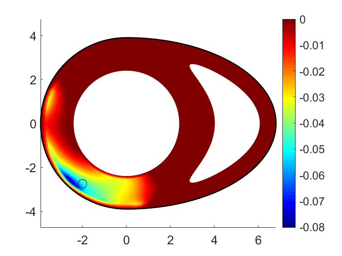 Figure 3
 Figure 4
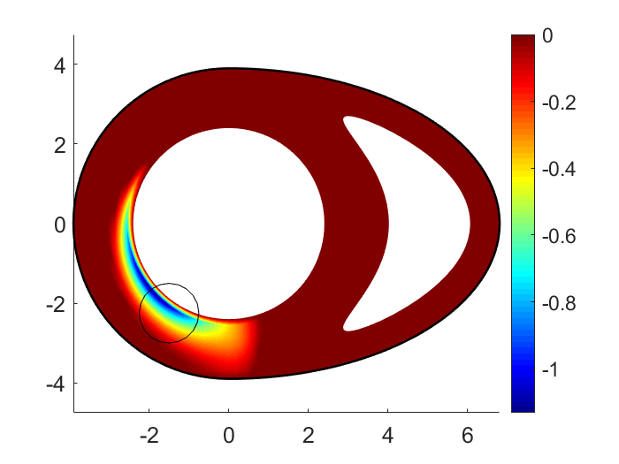 Figure 5
 Figure 6
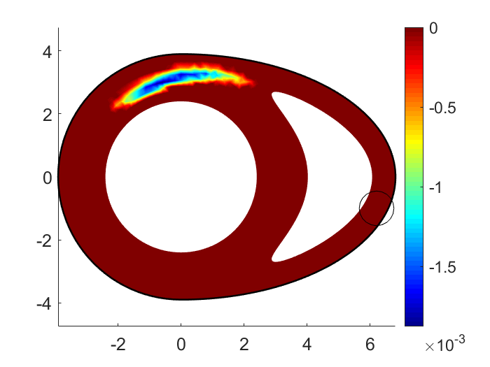 Figure 7
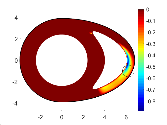 Figure 8
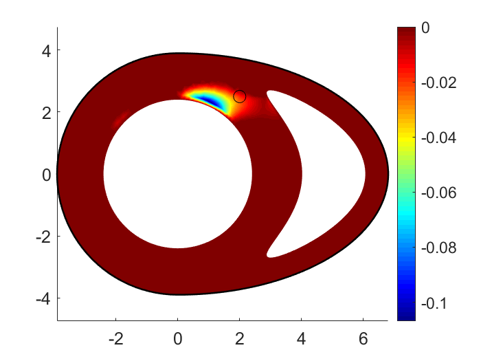 Figure 9
 Figure 10
 Figure 11
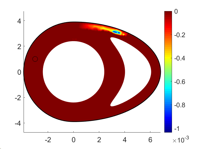 Figure 12
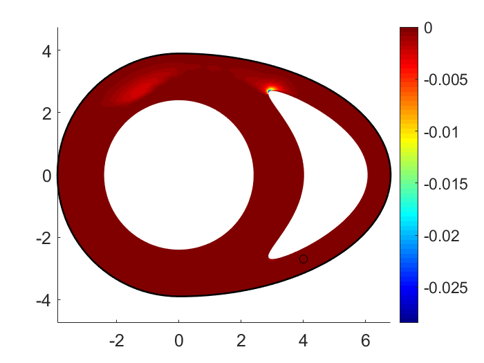 Figure 13
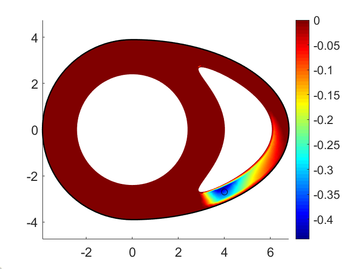 Figure 14
 Figure 15
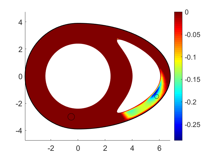 Figure 16
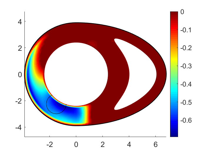 Figure 17
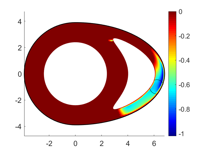 Figure 18
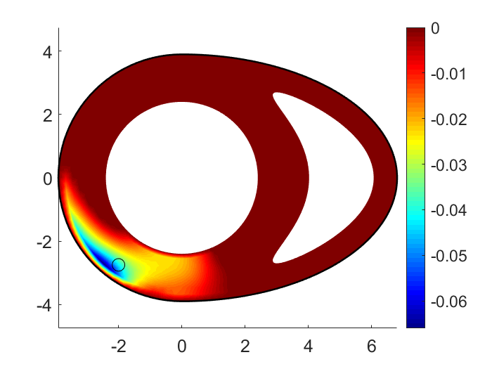 Figure 19
 Figure 20
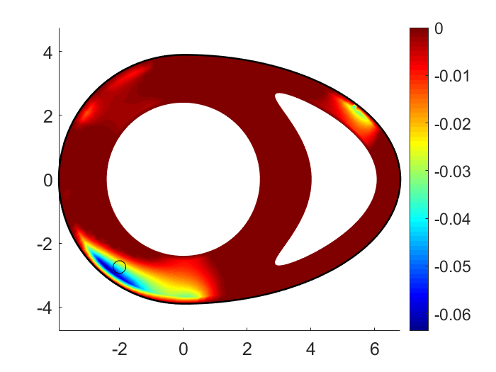 Figure 21
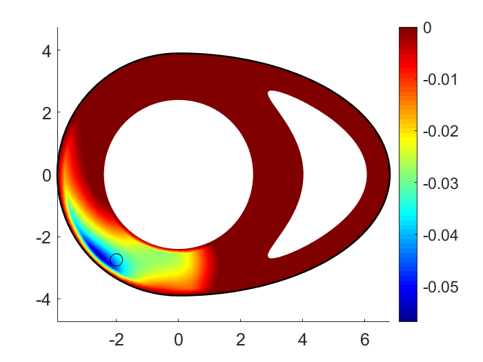 Figure 22
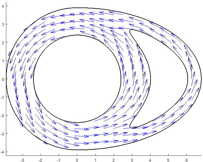 Figure 23
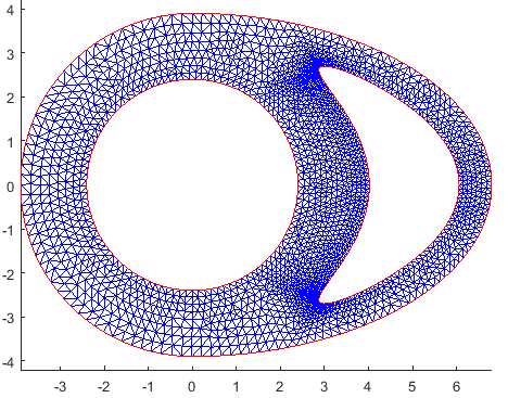 Figure 24
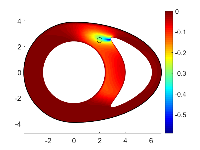 Figure 25
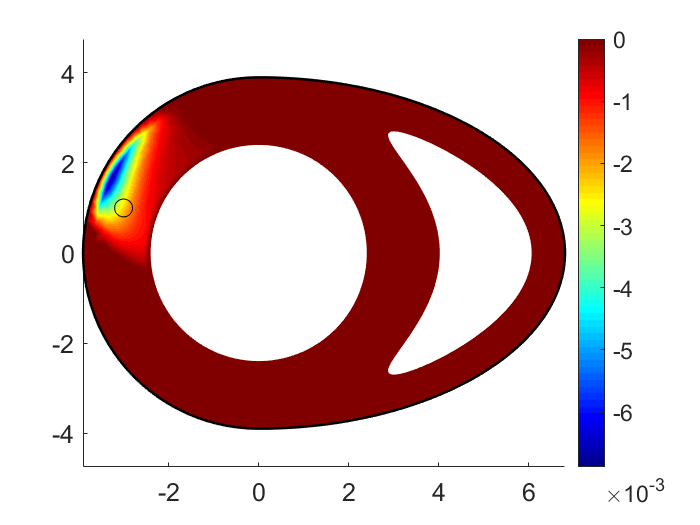 Figure 26
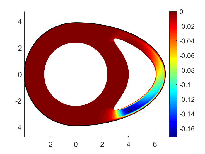 Figure 27
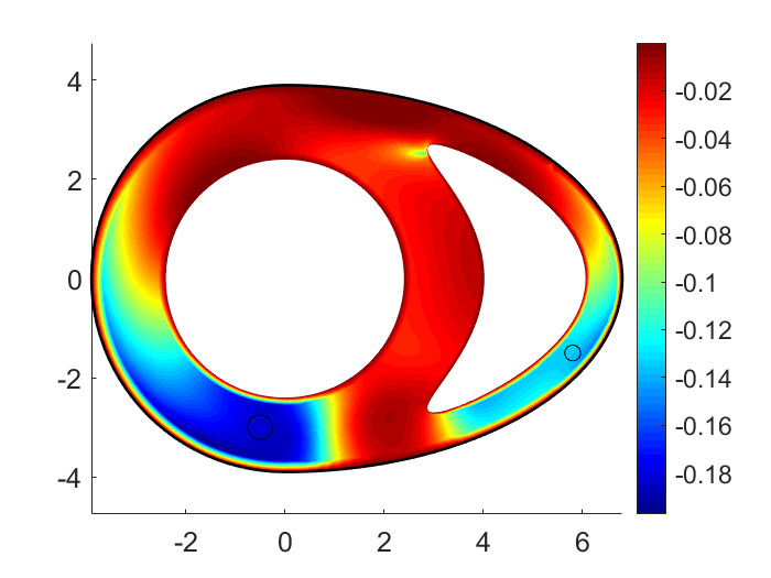 Figure 28
Peer Reviews
No public reviews on file for this paper yet. If you reviewed it on a platform where reviews are public (OpenReview, ICLR, NeurIPS, ICML), you can paste yours below so the community can read it here.
Videos
No videos yet. Explain this paper in a talk, walkthrough, or lecture? Add one.
On the determination of ischemic regions in the monodomain model of cardiac electrophysiology from boundary measurements
Elena Beretta111NYU Abu Dhabi (UAE), Politecnico di Milano (Italy) [email protected], [email protected], Cecilia Cavaterra222Università degli Studi di Milano (Italy), IMATI-CNR (Italy) [email protected], Luca Ratti333University of Helsinki (Finland) [email protected]
Abstract
In this paper we consider the monodomain model of cardiac electrophysiology. After an analysis of the well-posedness of the model we determine an asymptotic expansion of the perturbed potential due to the presence of small conductivity inhomogeneities (modelling small ischemic regions in the cardiac tissue) and use it to detect the anomalies from partial boundary measurements. This is done by determining the topological gradient of a suitable boundary misfit functional. The robustness of the algorithm is confirmed by several numerical experiments.
1 Introduction
Cardiac ischemia consists in a restriction of blood supply to the heart tissue usually caused by atherosclerosis or coronary syndrome. The shortage of oxygen may lead to dysfunction of the cell metabolism and eventually to their death. The possible outcomes range from ventricular arrhythmia, fibrillation and ultimately to myocardial infarction.
The ischemic heart syndrome is the most common cardiovascular disease, and the most common cause of death. Hence, the detection of ischemic regions at early stage of their development is of primary importance. This is usually performed by imaging techniques such as echocardiography, gamma ray scintigraphy or magnetic resonance imaging. Nevertheless, the most common test for patients not exhibiting evident symptoms is the electrocardiogram (ECG), which consists in recording electrical impulses across the thorax by means of a set of electrodes. Physicians are often able to identify myocardial ischemia by analysing the evolution of the voltage recorded in the ECG leads although with several technical difficulties (see the mathematical studies in [29] and [10]).
The approach we propose in this paper is to obtain information regarding the electrical functioning of the tissue (and ultimately the presence of ischemic regions) from the knowledge of the electrical potential on the surface of the heart. When employing the potential on the epicardium, i.e., the external boundary of the heart, this can be considered as a natural extension of the well-known mathematical problem often referred to as the inverse problem of electrocardiography, which consists in using the ECG recordings to compute the potential distribution on the epicardium. Alternatively, we remark that it is also possible to obtain electrical measurements on the endocardium, namely the internal boundaries of the heart cavities. Although much more invasive than the ECG, intracardiac ECG (iECG) has become a standard of care in patients with symptoms of heart failure, and allows to get a map of the endocardiac potential by means of non-contact electrodes carried by a catheter inside a heart cavity. We therefore assume that the distribution of the electrical potential is available on some portion of the heart boundary (on the epicardium, in the case of ECG data, or on the endocardium, in the case of iECG measurements). After a reliable model is introduced for the description of the evolution of the electrical potential within the heart, the problem of detecting ischemic regions is hence formulated as an inverse boundary value problem of identifying parameters in a nonlinear reaction diffusion system from boundary data.
In this paper we focus on the determination of small ischemias from boundary measurements of the electrical potential, generalizing the results obtained in previous papers (see [8],[6],[9]) to the monodomain time-dependent model of cardiac electrophysiology.
In general, this model is described by a system consisting in a semilinear parabolic equation coupled with a system of nonlinear ordinary differential equations, where the state variables are the transmembrane potential across the cell membrane, the concentrations of ionic species and the gating variables describing the activity of ionic channels in the membrane. It is well known (see [15] and [11]) that the monodomain model can be derived from the more complex bidomain one, introduced for the first time in [36], for instance by assuming proportionality between intracellular and extracellular conductivity tensors. In particular, in this case, the corresponding conductivity tensor becomes the harmonic mean of the extra and intracellular conductivities. On the other hand, this choice of the conductivity tensor turns out to be the best one to approximate the electrical propagation described by the bidomain model (see, e.g., [28],[16]).
As a first attempt, we limit ourselves to analyze a coupled system of two equations in the potential and the recovery variable . This corresponds to a large class of phenomenological models, which are characterized by the choice of the nonlinear terms appearing in the partial differential equation and in the ordinary differential equation. Among the most important two-equation systems (see [15] for a general overview) we mention FitzHugh-Nagumo, Rogers-McCulloch and Aliev-Panfilov models. Throughout this paper, we focus on the commonly used version of the Aliev-Panfilov model (originally introduced in [1]), even though the analysis could be extended also to the other two.
In order to detect ischemic regions, we extend the approach of [9], determining a rigorous asymptotic expansion for the perturbed boundary potential due to small conductivity anomalies. To accomplish this task, we need an accurate analysis of the well-posedness of the direct problem for the coupled system in the case of discontinuous anisotropic coefficients and suitable regularity estimates for solutions. In particular, we establish a comparison principle for this class of systems, which to our knowledge was not present in the literature. Here, we consider the case of an insulated heart and we assume to have measurements of the potential on a portion of the boundary.
The theory of detection of small conductivity inhomogeneities from boundary measurements via asymptotic techniques has been developed in the last three decades in the framework of Electrical Impedance Tomography (see, e.g., [3],[14],[5]). A similar approach has also been used in Thermal Imaging (see, e.g., [4]). Here, we are able to extend in a non trivial way the results obtained previously in [6] and [9] for simplified versions of the monodomain model making use of fine regularity for the solutions to nonlinear reaction diffusion systems. In particular, we establish a rigorous expansion for the perturbed transmembrane potential and use this to implement an effective reconstruction algorithm.
The paper is organized as follows. In Section 2 we analyze the well-posedness of the forward problem in the unperturbed and perturbed case. Section 3 is devoted to obtaining energy estimates on the difference between the perturbed and unperturbed electrical potential and an asymptotic expansion of suitable integral terms involving such difference on the boundary. In Section 4 we describe our topological-based optimization algorithm and derive rigorously the topological gradient of a suitable mismatch functional. This is obtained by using the results of Section 3 and some interior regularity results for the solution of parabolic systems. Finally, in Section 5 we outline the numerical implementation of the proposed algorithm, relying on the Finite Element Method for the discrete formulation of the problem. A significant set of numerical experiments is provided in order to assess the effectiveness of the reconstruction, even in presence of data noise.
2 Analysis of the direct problem
The well-posedness analysis of the monodomain system has been object of several studies. We refer to [15, Chapter 3] for a general overview. In [12] a result of existence and uniqueness of weak solution is proved for the FitzHugh-Nagumo, the Aliev-Panfilov and the Rogers-MacCulloch models by means of a Faedo-Galerkin procedure. A result of existence of strong solutions, local in time, is also derived. In [37], instead, results of well-posedness are obtained for a wider range of models, on the base of a fixed point argument.
Regarding the regularity of the solutions of the monodomain system, we report a result in [17] for FitzHugh-Nagumo, Aliev-Panfilov and Rogers-MacCulloch models: if no discontinuities are present in the coefficients of the system, existence and uniqueness of strong solutions is guaranteed, locally in time (see for instance [34] and [20]). A comparison principle is also provided, by means of the tool of invariant sets, allowing to prove existence of global solutions. We also report a result of local existence of classical solutions for the bidomain model, recently obtained in [19].
In this section we focus on the monodomain system in the case of smooth diffusion coefficient and reaction term, corresponding to the case of the healthy tissue (unperturbed case) and in the case of discontinuities in the diffusion coefficient and in the reaction term, corresponding to the presence of an ischemia in the heart tissue (perturbed case). We state an existence, uniqueness and comparison result for classical solutions of the unperturbed case (a proof of which, alternative to the approach of [17], is proposed in [31, Chapter 6]) and prove a result regarding existence, uniqueness and regularity of weak solutions in the perturbed case.
In particular, the initial and boundary value problem associated to the unperturbed monodomain system is the following one
[TABLE]
where is the region occupied by the hearth tissue, is the outward unit normal vector to the boundary , and . A slightly different formulation of the monodomain model (see, e.g., [15]) involves the presence of a source term in the right-hand side of the first equation in (2.1), representing an applied current, during a limited time window (the initial activation of the tissue). We replace the effect of such a current with the presence of a non-null initial value . Since the modeling differences between the two formulations are negligible after the first instants, we choose the one proposed in (2.1) more suited for the mathematical analysis of the problem.
In presence of an ischemia , the perturbed case is described by the model
[TABLE]
where is the indicator function of and . We now specify the requirements on the domain, the coefficients and the source terms.
Assumption 1**.**
* bounded domain, , and ;* 2. 2.
the inclusion is well separated from the boundary, i.e.,
[TABLE] 3. 3.
* are symmetric matrix-valued functions in ; , the matrices and admit positive eigenvalues and respectively, associated to the same eigenvectors such that ;* 4. 4.
, , and on ; 5. 5.
we assume as in the Aliev-Panfilov model, namely:
[TABLE]
being and .
Remark 1**.**
The requirements on the matrix-valued functions and are satisfied by the conductivity tensors prescribed in the model under consideration (see [15, 35]). According to experimental evidence, the cardiac tissue can be modeled as an orthotropic material, characterized by the presence of fibers and sheets, which define the conductivity eigenvectors. Moreover, the presence of an ischemia does not affect the direction of the fibers, but reduces the value of all the associated eigenvalues. From now on, we will indicate by the minimum eigenvalue of and by the maximum eigenvalue of .
Remark 2**.**
As an immediate consequence of (2.4), and satisfy the Tangency condition on the rectangle , (see [2]), i.e., indicating by a generalized outward normal on ( for all , is such that ) then,
[TABLE]
Moreover, the functions are Lipschitz continuous on with constants .
Remark 3**.**
For the sake of brevity, in all the formulas we avoid to indicate time and space integration variables with respect to the classical Lebesgue measure, unless it is necessary.
We now outline the main results regarding the well-posedness of the problems (2.1) and (2.2).
Theorem 1** (Unperturbed problem).**
Let Assumption 1 holds, and suppose that, . Then, problem (2.1) admits a unique classical solution , namely , . Moreover, , for each .
The proof of Theorem 1 is derived by means of classical fixed point argument (see [27, Chapter 8, Sections 9 and 11]). A detailed proof is reported in [31, Theorem 6.1].
Regarding the perturbed problem (2.2), we note that, although the conductivity tensor and the nonlinear term are discontinuous, we can extend the results obtained in [12] thanks to the uniform ellipticity to the boundedness of the conductivity tensors and to the form of the reaction term, deriving the following existence and uniqueness result.
Theorem 2** (Perturbed problem).**
Let the Assumption 1 holds, and suppose that, . Then, problem (2.2) admits a unique weak solution, i.e., a couple such that , , , and satisfying, for a.e. ,
[TABLE]
Moreover, , and , .
Proof.
To start with, note that uniqueness of the weak solution of (2.2) has been shown in the case of Aliev-Panfilov model in [21, Theorem 1.3] as a byproduct of a stability result obtained by exploiting the specific nonlinear expression of and .
We proceed now introducing a sequence of regularized problems of (2.2) and showing that the sequence of their solutions converges to a weak solution of (2.2). We then exploit additional properties inherited by the approximation process to conclude the stated regularity results. The uniqueness argument is briefly sketched.
Since is an indicator function, surely ; by density arguments and according to (2.3),
[TABLE]
being the space of functions with compact support in . Define and let be the solution of the following problem
[TABLE]
where we have used the fact that on . We observe that, for any fixed , an application of Theorem 1 ensures the existence and uniqueness of a classical solution of Problem (2.8). Moreover by (2.7) we have that and satisfy the Tangency condition on . Hence, from Theorem 1 we deduce , for all .
We now prove that from the convergence of to a weak solution of (2.2) holds. We start by proving some a priori estimates. Consider the weak form of the problem solved by and take the classical solutions , as test functions. Then, we get
[TABLE]
Recall now that is the minimum eigenvalue of , whereas is the maximum eigenvalue of . Moreover, since , , are uniformly bounded independently of (indeed, and ) and are continuous, we can introduce and , which are independent of . Hence, by Young inequality,
[TABLE]
Using Gronwall’s inequality, we get
[TABLE]
which implies
[TABLE]
Integrating from [math] to (2.9) and using last estimate it also follows that
[TABLE]
A bound for the norm of can be found by considering that, for each ,
[TABLE]
and computing the norm in time
[TABLE]
Analogously, one proves that , with independent of .
As a consequence of the uniform bounds we can ensure that (up to a subsequence) , , , such that
[TABLE]
Using the result contained in [33, Theorem 8.1] and the uniqueness of the weak solution of the perturbed problem we have that (see [33, Theorem 8.1]), hence a.e. in . Moreover, also a.e. in as it can be straightforwardly obtained by the expression
[TABLE]
Consider now the weak form of the problem solved by : , .
[TABLE]
Taking the limit in , exploiting the weak convergence of , , , , we obtain that , in and that the limit satisfies, , ,
[TABLE]
Indeed, the convergence of the terms involving the time derivatives is a direct consequence of the weak convergence of , and of the definition of distributional derivative. The limit of the nonlinear reaction terms can be proved by taking advantage of the dominated convergence theorem and of the pointwise (a.e.) convergence of and . The convergence of the diffusion term is obtained by combining the weak convergence of in , the pointwise (a.e.) convergence of and the uniform bound on . According to (2.12), we can ensure that the limit is the weak solution of (2.2).
The weak solution is moreover a pointwise (a.e.) limit of the regularized solutions . As a consequence, the uniform bound on is valid also for the limit: a.e. in . This allows to prove the additional Hölder regularity of . Indeed, since , , we can apply Theorem 10.1 of [22, Chapter 3] on the first equation in (2.2)
[TABLE]
to get . Now, we can extend the regularity result up to the boundary due to the hypothesis on and on contained in Assumption 1, and conclude . Using the analytic expression of that can be obtained by (2.10) and the regularity of , we can also deduce that . ∎
3 Analysis of the inverse problem
We now tackle the inverse problem of identifying a perturbation from boundary measurements. Suppose to know , the trace of the solution of (2.2) in presence of an unknown inclusion. The inverse problem reads
[TABLE]
Although the analysis of the direct problem has been performed in presence of an arbitrary inclusion , for the purpose of solving the inverse problem and derive a reconstruction algorithm, we limit ourselves at considering the case of inclusions of small size, in analogy to what done in [8], [9]. In particular, we consider a family of inclusions satisfying (2.3) for each and such that
[TABLE]
We define the indicator function of , and the solution of problem (2.2) with , in the sense of Theorem 2.
3.1 Energy estimates
We now derive some energy estimates for the difference between and , the solution of the unperturbed problem (2.1) in terms of when .
From now on we will indicate by a positive constant depending on the data, independent of and that may vary also in the same line.
Proposition 1**.**
Under Assumption 2.1 the following inequalities hold
, , .
Proof.
We consider (2.6) with and the weak formulation of the unperturbed problem (2.1). Subtracting term by term and defining and , we have that , and, for almost every ,
[TABLE]
Let , then, according to Theorem 1 and Theorem 2, both and range within the rectangle , on which the functions and are Lipschitz continuous with constants less or equal than . Hence
[TABLE]
Via an application of Schwarz and Young inequalities on the last two terms in the right-hand side of the previous inequality, and from the regularity of the solution , we can deduce
[TABLE]
An application of Gronwall’s lemma to (3.4) entails that , and ultimately can be bounded by . This allows to conclude the first two statements.
Observe now that the pair is also the solution of
[TABLE]
By the mean value theorem, there exist two pairs of functions , s.t. ***it follows by an application of the Lagrange’s mean value theorem on the real-valued function on the interval ; the same holds for .
[TABLE]
By definition, and are convex combinations of and , thus they assume values in the rectangle . Let now be the solution of the adjoint problem
[TABLE]
with initial conditions , and homogeneous Neumann boundary condition. Consider the change of variable: , and define , , , and analogously for . Hence and solve
[TABLE]
Since and are bounded in , by standard Faedo-Galerkin technique we obtain that the solution of (3.7) exists and is unique with the properties , , , . Moreover
[TABLE]
Additional regularity of can be proved with an analogous argument as in [22, Chapter 4, Theorem 9.1], applied on the first equation in (3.7). Indeed, by the regularity of and the square integrability of , we can conclude that , and
[TABLE]
Moreover, multiplying the first two equations in (3.7) respectively by and and integrating on , straightforward computations allow to conclude that with
[TABLE]
By Sobolev inequality we obtain
[TABLE]
(all the norms being bounded by ; the same bounds hold on ). Thus, via Nirenberg interpolation estimates (see [25]), we get
[TABLE]
Recalling also the previous results, this allows to conclude that, taking ,
[TABLE]
Let us multiply the equations of (3.5) respectively by and the first two equations of (3.7) respectively by . Integrating on and summing the resulting identities it is easy to see that
[TABLE]
Thanks to (3.8) and Hölder inequality the first term of the right-hand side can be bounded as follows
[TABLE]
where and . In addition, again by Hölder inequality,
[TABLE]
Furthermore, it is straightforward to see that the last term in (3.9) can be bounded by . Finally, from (3.9) we conclude that, for ,
[TABLE]
Hence
[TABLE]
where . ∎
3.2 Asymptotic expansion of boundary voltage
In this section we prove the following result.
Theorem 3**.**
For every sequence with , , there exist a subsequence (still denoted by ), a Radon measure and a matrix-valued function such that, for every pair satisfying
[TABLE]
with the final conditions , , it holds
[TABLE]
In order to prove Theorem 3.11, we need to introduce the auxiliary functions , solving
[TABLE]
with and . By the choice of and it holds . Moreover, and satisfy the following energy estimates (see [13])
[TABLE]
We need also a preliminary lemma.
Lemma 1**.**
For each such that , we have, as ,
[TABLE]
Proof.
Since and are the solutions of problems (3.12), we obtain
[TABLE]
Take , being . By computation we get
[TABLE]
that we can rewrite as
[TABLE]
Proposition 1 and (3.13) lead to
[TABLE]
whereas,
[TABLE]
Collecting the previous two relations in (3.15), we conclude
[TABLE]
It can be easily verified that, for every , the following identities hold
[TABLE]
Taking in the first identity and in the second one, integrating in time and subtracting we obtain
[TABLE]
Via integration by parts, and taking advantage of the homogeneous initial and final conditions satisfied respectively by and it follows
[TABLE]
Analogous bounds can be proved for the last term in the left-hand side and the first term in the right-hand side of (3.17), thanks to the energy estimates of and the regularity of . As a consequence, it holds that
[TABLE]
In conclusion, by a combination of (3.16) and (3.18),
[TABLE]
which immediately entails the thesis. ∎
We are finally ready to prove the main result of this section.
Proof of Theorem 3.11.
Arguing as in [13], we deduce that there exist a Radon measure , a symmetric matrix and a sequence such that
[TABLE]
in the weak* topology of . Moreover, thanks to the regularity estimates for and the symmetries of the matrices , and , we have, for every ,
[TABLE]
which also implies
[TABLE]
in the weak∗ topology of .
On account of the energy estimates (3.13), straightforward computations show that for every there exists a constant , depending on the data and on but independent of , such that
[TABLE]
In particular, we define the limit measure in the weak∗ topology of ) as follows
[TABLE]
Exploiting (3.21) and (3.20), and recalling Lemma 3.3, we deduce
[TABLE]
and by the density of in we derive
[TABLE]
Now, setting and , and selecting and as test functions, we have
[TABLE]
Furthermore, since is a solution to (3.10), it also holds:
[TABLE]
Summing up the last two identities and integrating in time we observe that the terms involving the time derivatives vanish due to the initial and final conditions on . Consider now the non-linear terms containing
[TABLE]
Observe that by means of the Lagrange’s mean value theorem and the Lipschitz-continuity of the functions with constants we have
[TABLE]
whereas
[TABLE]
Analogous estimates can be obtained for the terms containing . Finally,
[TABLE]
Thanks to the regularity of , and employing the computed weak* limits, we derive
[TABLE]
which concludes the proof. ∎
4 Reconstruction algorithm: a topology optimization approach
The asymptotic expansion provided in Theorem 3.11 allows to describe the perturbation of the electrical potential on the boundary of the domain due to the presence of a small conductivity inhomogeneity . In order to derive a reconstruction algorithm for problem (3.1), we introduce the mismatch functional
[TABLE]
where solves the perturbed problem (2.2) in the presence of an ischemic region . We now prove that the functional restricted to the class of inclusions satisfying (2.3), (3.2) admits an asymptotic expansion with respect to the size of the inclusion. Moreover, as it is shown in Theorem 4.3, the first-order term of the expansion (which will be denoted as , the topological gradient of ) can be computed by solving the unperturbed problem and a suitable adjoint problem. In particular, we restrict ourselves to inclusions satisfying (2.3) and of the form
[TABLE]
where is a bounded, smooth set containing the origin.
We have the following
Theorem 4**.**
Consider a family satisfying (2.3) and (4.2). Then, there exists a matrix (which may depend on , , and ) such that, as ,
[TABLE]
where solves (2.1) and is the solution of the adjoint problem:
[TABLE]
Proof.
First of all, we note that, since Lemma 3.3 holds under the weaker assumption on the test functions, , then the validity of Theorem 3.11 can be easily extended when . We now show that the solution to (4.3) enjoys this regularity. In fact this can be ensured by a lifting argument, since the boundary datum . Estimates of the norm of can be obtained by flattening the boundary and by reflection arguments, see for example [22, Chapter 7, Theorem 2.2] for a two-dimensional case.
It is straightforward to verify that
[TABLE]
The first term in the right-hand side of (4.4) involves the boundary condition of the adjoint problem, and in particular it can be written as . We now apply Theorem 3.11 in order to conclude that
[TABLE]
According to assumption (4.2), the limit measure is independent of the choice of the subsequence and is equal to , the Dirac measure centered in . Finally, the second term in the right-hand side of (4.4) is by means of Lemma 2 below. ∎
Remark 4**.**
By Assumption 2.1 and by the homogeneous boundary conditions on we can conclude, using standard local regularity results on parabolic equations applied in a neighbourhood of , that
Lemma 2**.**
Let satisfy (2.3) and (4.2). Then,
[TABLE]
Proof.
By the same argument as in the proof of Theorem 4.3 and by Remark 4.2,
[TABLE]
where satisfies
[TABLE]
and .
We now focus on proving that for a compact set such that and satisfying one has
[TABLE]
and, as a consequence of a Sobolev immersion, (4.6) implies (here )
[TABLE]
By a combination of (2.3) and (4.2) we can ensure that the support of the measure is contained in . This would entail that
[TABLE]
hence .
In order to prove (4.6), by standard Faedo-Galerkin technique applied to the linear system (4.5), one has
[TABLE]
Moreover, according to (4.5), is the solution of the following problem
[TABLE]
Analogously to what stated in [22, Chapter 4, Theorem 9.1], it holds that
[TABLE]
and in conclusion, by the regularity of and by (4.7)
[TABLE]
Similar estimates can be derived also for since and . This last property is guaranteed on by Theorem 1, whereas it can be extended to since we consider . Now, by computing the solution of the third equation in (4.5) in closed form, we can easily verify that
[TABLE]
Consider the change of variable and denote by . We now focus on the first equation in (4.5) and compute the second derivatives of each term. Then, satisfies the following equation in a weak sense:
[TABLE]
being
[TABLE]
Let be an open subset of , such that . By interior regularity results it holds that is smooth on , which entails by the initial conditions that
[TABLE]
According to the smoothness of and to the bounds (4.8) and (4.9), we get
[TABLE]
In fact, all the terms in except the first three belong to , with norm bounded by or by . Set , then, for any ,
[TABLE]
where indicates the duality pairing between the involved spaces. Integrating in time last relation we finally get
[TABLE]
With similar arguments we can estimate also the second and third term in the definition of the function leading finally to (4.12).
Consider now a test function , , such that in . According to (4.10), by simple computations we verify that satisfies
[TABLE]
being . It holds that , and
[TABLE]
hence we observe that
[TABLE]
By standard Faedo-Galerkin argument (see, e.g., [18, Chap. 18, Par. 3, Theorem 3], we verify that
[TABLE]
Finally, by the definition of , combining (4.15) and (4.14) we conclude that
[TABLE]
The thesis is now proved thanks to the trace inequality and the energy estimates. ∎
Theorem 4.3 gives a representation formula for the topological gradient , the first order term in the expansion of the mismatch functional . In analogy to [6, 9], we propose a one-step reconstruction Algorithm 1 for the identification of small inclusions satisfying (4.2).
Remark 5**.**
The polarization tensor can be computed in an explicit form, e.g., when the shape of the inclusion is a disk, even though it is not straightforward in the current anisotropic case. Since depends on and and on the shape of the set , which we assume to be a disk, it varies according to the space variable . In order to compute , we first use [3, Lemma 4.30] to transform and in diagonal matrices. By a rescaling of the spatial variables, we can reduce to the case in which one of the two diagonalized tensors is the identity, which allows to apply [3, Proposition 4.31]. We remark that the anisotropic rescaling entails that the original circle is transformed in an ellipse of known semiaxes.
5 Numerical results
In this section we describe the implementation of Algorithm 1 and report some numerical results in order to show its effectiveness. In particular, we set our experiments in a two-dimensional idealized geometry, representing a horizontal section of the ventricles. The application of the model on a three-dimensional geometry would be equivalently possible, and will be object of future studies, employing advanced numerical analysis techniques in order to tackle the increased computational effort. We rely on synthetic data, i.e., we solve the monodomain system in presence of a prescribed ischemic region and then use the value of the solution on the boundary (or a portion of it) as an input for the reconstruction algorithm. In order to prevent inverse crimes, we employ different numerical settings for the synthetic data generation and for the solution of the unperturbed and adjoint problems, required for the reconstruction algorithm. In particular, we adopt a much more refined discretization, both in space and in time, for the simulation of the synthetic data.
In the following experiments we assume to measure the voltage only on a portion of the heart. As outlined in Section 1, measurements of the voltage can be acquired on the inner surface of a ventricle by intracavitary measurements, or, alternatively, we might be able to compute a map of the electrical potential on the epicardium starting from ECG data. This does not affect the reconstruction procedure described in Algorithm 1, apart from the definition of the adjoint problem (4.3), which now prescribes oblique boundary conditions involving on the portion of the boundary where the measurements are acquired, and homogeneous Neumann conditions elsewhere.
5.1 Finite Element approximation
In order to numerically approximate the solution of the monodomain model, we rely on a Galerkin Finite Element scheme, introducing a tessellation of the domain consisting of triangular elements. In particular, we adopt two different meshes for the solution of the unperturbed (and adjoint) problem and for the generation of the synthetic measurements, the latter being more refined especially close to the boundary of the prescribed ischemic region.
Moreover, in order to reproduce the anisotropic behavior of the conductivity coefficients and , we consider the presence of fibers within the domain. We adopt a procedure analogous to the one reported in [30] for the generation of the fiber directions, resorting on the solution of a Laplace problem with suitable boundary conditions. Once the direction of the fibers is defined within , as well as the transmural vector field (obtained by a clockwise rotation of of ), the definition of the conductivity tensors is
[TABLE]
The numerical mesh for the solution of the background problem and the directions of the fibers are reported in Figure 1.
As already mentioned in the introduction, the best choice of the conductivity tensor to be employed in the numerical simulations of the monodomain model is given by the harmonic mean of the intracellular and extracellular conductivity tensors and appearing in the bidomain model that can be expressed by
[TABLE]
Exploiting the fact that and have the same eigenvectors (again defined by the fiber and transmural directions), we can therefore compute the eigenvalues of (and analogously of ) as the harmonic mean of the ones of and as reported, e.g., in [15, Table 8.1]. The values of the main parameters involved in the numerical simulations are reported in Table 1.
The numerical solution of the background problem (2.1) relies on a Newton-Galerkin scheme. The spatial discretization is performed thanks to the P1-finite element space, i.e., the space of the continuous functions over which are linear polynomials when restricted on each element of the mesh. The temporal discretization is done via an implicit Euler scheme. This leads to solve a nonlinear problem at each timestep, which is performed via a Newton iterative algorithm. More details on the solver can be found in [32], where a thorough convergence analysis is performed.
5.2 Reconstruction of small inclusions
We study the effectiveness of the reconstruction algorithm in identifying the position of small ischemic regions within the cardiac tissue. For, we employ synthetic measurements of the perturbed boundary voltage in presence of ischemias located in different sections of the cardiac tissue: in the left ventricle, in the septum, or in the right ventricle. In each simulation, we consider circular ischemic regions of radius ranging from to . In Figure 2 we report the contour plot of the topological gradient in four different cases, and superimpose a black line representing the boundary of the ischemia that we aim to reconstruct.
From an analysis of Figure 2 we can deduce that the topological gradient always attains its negative minimum value close to the real position of the ischemia, and the accuracy of the localization may vary according to the position of the ischemia. We achieve significant results also in the case of multiple inclusions. When more than one ischemic region is present, the topological gradient shows a local minimum close to each region. As depicted in the captions, some experiments employ the knowledge of the voltage on the epicardium and some on one endocardiac surface. The reconstruction appears fairly accurate in both cases. We remark that the algorithm is always effective when using epicardiac measurements, but fails in detecting ischemic regions located in a ventricle whenever the measurements are acquired on the inner surface of the other one. Nevertheless, even in those cases the technique avoids false positive detection, i.e., the topological gradient does not show significant local minima in wrong locations.
5.3 Reconstruction from noisy measurements
We now focus on the performance of the algorithm in presence of noisy measurements, in order to assess the stability of the algorithm with respect to small perturbations of the boundary data of the form
[TABLE]
where is a standard Gaussian random variable for each point and instant , and is the noise level.
In Figure 3 we report the contour plot of the topological gradient computed with noiseless measurements and compare it with the ones obtained with growing levels of noise. The algorithm shows to be stable even under significantly corrupted measurements: up to the level , the negative region in correspondence to the exact position is clearly identifiable.
5.4 Reconstruction of large inclusions
We eventually remark that the proposed algorithm produces significant results also when applied to measurements associated to large ischemic regions. The identification of larger regions could be performed by means of iterative reconstruction algorithms, as the one proposed in [7] for a semilinear elliptic problem. Nevertheless, as it is shown in Figure 4, the information coming from the topological gradient could be a suitable initial guess for such iterative algorithms.
6 Conclusions
In this paper, we have studied the identification of small ischemic regions in the cardiac tissue, represented by discontinuous alterations in the conductivity and in the nonlinear reaction term of the monodomain model, taking advantage of the measurement of the voltage on the boundary of the heart. We have extended the existing results regarding the well-posedness of the direct problem and derived a rigorous asymptotic expansion of the perturbed boundary voltage, which allows to formulate an effective reconstruction algorithm based on topological optimization.
We foresee several significant extensions of the presented analysis, both from an analytical and a numerical viewpoint. The coupling of the monodomain model of the heart with a passive conductor model for the surrounding torso (see [11]) would enable us to make use of ECG data for reconstruction purposes, possibly comparing the results with the ones obtained in [23],[38] with a stationary version of the bidomain model.
The effectiveness of the reconstruction algorithm should also be tested in a three-dimensional setting; in such a context, due to the high computational cost of the numerical simulation, a Reduced Order Modeling approach could be considered, as recently analysed in [26].
Finally, the detection of arbitrarily large ischemic regions can be tackled, exploiting an analogous strategy as the one adopted in [6] (possibly reducing the computational effort by employing an adaptive solver of the monodomain system, as proposed in [32]).
Acknowledgments
The authors are grateful to Roberto Gianni for his useful suggestions. The authors thank the New York University of Abu Dhabi for its kind hospitality. The work of the authors has been supported by GNAMPA (Gruppo Nazionale per l’Analisi Matematica, la Probabilità e le loro Applicazioni). The numerical simulations presented in this work have been performed thanks to the MATLAB library redbKIT, [24].
The reference list from the paper itself. Each links out to its DOI / PubMed record.
- 1[1] R.R. Aliev and A.V. Panfilov “A simple two-variable model of cardiac excitation” In Chaos, Solitons & Fractals 7.3 , 1996, pp. 293–301
- 2[2] H. Amann “Invariant sets and existence theorems for semilinear parabolic and elliptic systems” In Journal of Mathematical Analysis and Applications 65.2 Academic Press, 1978, pp. 432–467
- 3[3] H. Ammari and H. Kang “Reconstruction of small inhomogeneities from boundary measurements”, Lectures Notes in Mathematics Series, Volume 1846 Springer, 2004
- 4[4] H. Ammari, E. Iakovleva, H. Kang and K. Kim “Direct algorithms for thermal imaging of small inclusions” In Multiscale Modeling & Simulation 4.4 SIAM, 2005, pp. 1116–1136
- 5[5] H. Ammari, J. Garnier, V. Jugnon and H. Kang “Stability and resolution analysis for a topological derivative based imaging functional” In SIAM Journal on Control and Optimization 50.1 SIAM, 2012, pp. 48–76
- 6[6] E. Beretta, A. Manzoni and L. Ratti “A reconstruction algorithm based on topological gradient for an inverse problem related to a semilinear elliptic boundary value problem” In Inverse Problems 33.3 IOP Publishing, 2017, pp. 035010
- 7[7] E. Beretta, L. Ratti and M. Verani “Detection of conductivity inclusions in a semilinear elliptic problem arising from cardiac electrophysiology” In Communications in Mathematical Sciences 16.7 International Press of Boston, 2018, pp. 1975–2002
- 8[8] E. Beretta, M.C. Cerutti, A. Manzoni and D. Pierotti “An asymptotic formula for boundary potential perturbations in a semilinear elliptic equation related to cardiac electrophysiology” In Math. Mod. and Meth. in Appl. S. 26(04) , 2016, pp. 645–670