Depth-based Weighted Jackknife Empirical Likelihood for Non-smooth U-structure Equations
Yongli Sang, Xin Dang, Yichuan Zhao

TL;DR
This paper introduces a weighted jackknife empirical likelihood method to improve robustness against outliers in non-smooth U-structure equations, providing theoretical properties and demonstrating effectiveness through simulations and real data.
Contribution
It proposes a novel weighted JEL approach that reduces outlier sensitivity and derives its asymptotic distribution, enhancing robustness in non-smooth U-statistic problems.
Findings
WJEL converges to a scaled chi-square distribution.
Self-normalized WJEL yields standard chi-square distribution.
Simulation studies confirm robustness against outliers.
Abstract
In many applications, parameters of interest are estimated by solving some non-smooth estimating equations with -statistic structure. Jackknife empirical likelihood (JEL) approach can solve this problem efficiently by reducing the computation complexity of the empirical likelihood (EL) method. However, as EL, JEL suffers the sensitivity problem to outliers. In this paper, we propose a weighted jackknife empirical likelihood (WJEL) to tackle the above limitation of JEL. The proposed WJEL tilts the JEL function by assigning smaller weights to outliers. The asymptotic of the WJEL ratio statistic is derived. It converges in distribution to a multiple of a chi-square random variable. The multiplying constant depends on the weighting scheme. The self-normalized version of WJEL ratio does not require to know the constant and hence yields the standard chi-square distribution in the limit.…
Click any figure to enlarge with its caption.
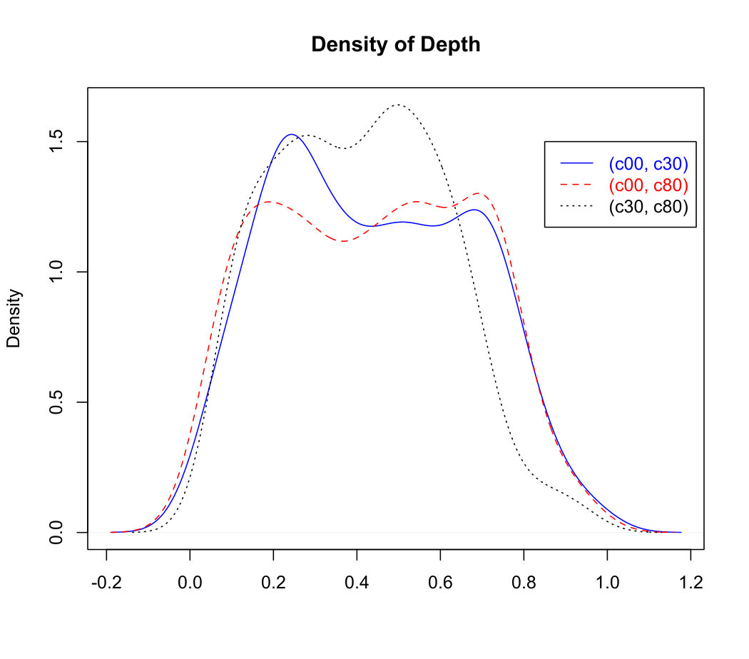 Figure 1
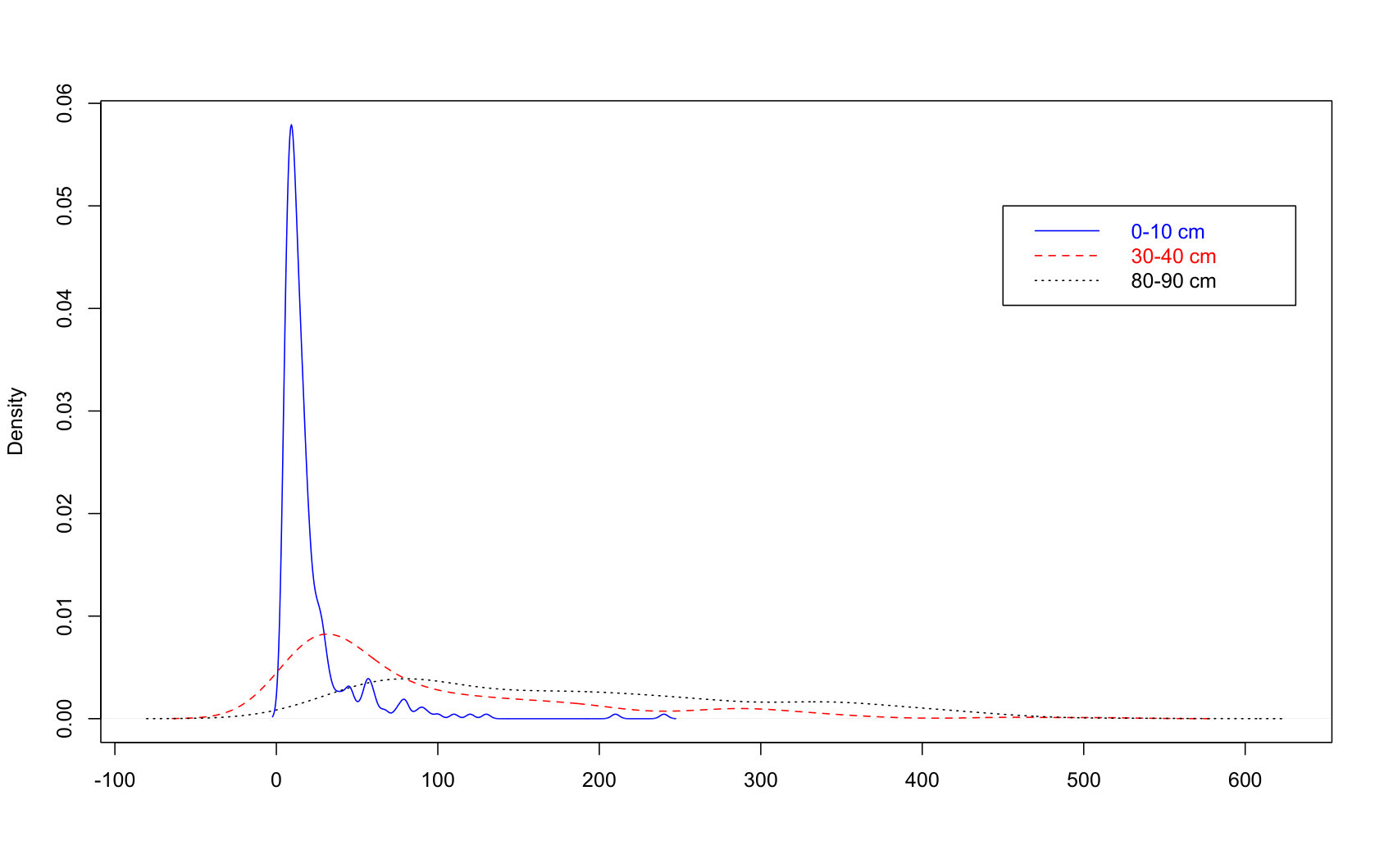 Figure 2
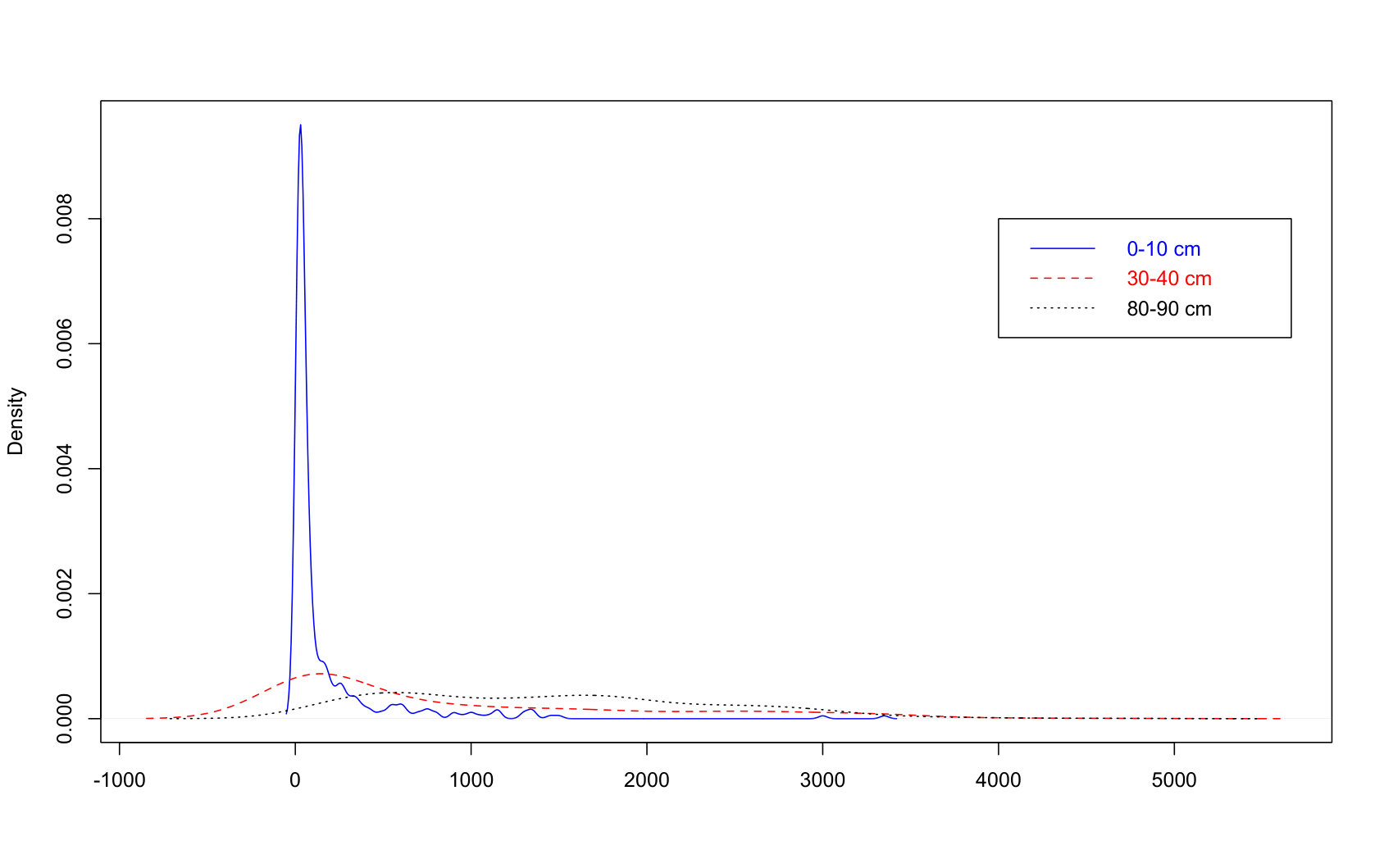 Figure 3
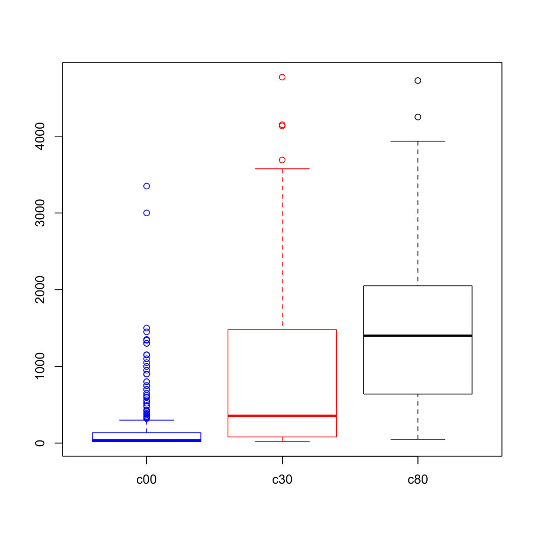 Figure 4
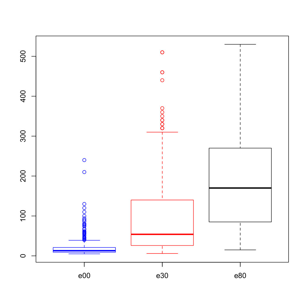 Figure 5
| Contamination levels | Method | |||
|---|---|---|---|---|
| CovProb Length | CovProb Length | |||
| JEL | .929(.007) .840(.011) | .951(.009) .338(.003) | ||
| WJEL | .948(.005) 1.02(.008) | .936(.012) .398(.003) | ||
| JEL | .929(.005) .842(.006) | .948(.009) .338(.003) | ||
| WJEL | .948(.005) 1.02(.009) | .932(.010) .398(.003) | ||
| JEL | .927(.007) .689(.006) | .948(.010) .364(.003) | ||
| WJEL | .944(.005) .839(.010) | .934(.009) .325(.003) | ||
| JEL | .925(.007) .688(.008) | .947(.006) .364(.002) | ||
| WJEL | .943(.005) .840(.010) | .934(.010) .326(.003) | ||
| JEL | .921(.009) .247(.004) | .945(.007) .099(.001) | ||
| WJEL | .942(.010) .254(.004) | .928(.008) .091(.001) | ||
| JEL | .915(.010) .246(.003) | .946(.007) .099(.001) | ||
| WJEL | .938(.010) .254(.003) | .928(.008) .091(.001) | ||
| JEL | .923(.006) .865(.009) | .945(.009) .363(.002) | ||
| WJEL | .946(.007) 1.05(.007) | .940(.010) .414(.003) | ||
| JEL | .922(.009) .864(.009) | .945(.010) .363(.002) | ||
| WJEL | .948(.008) 1.05(.007) | .940(.012) .414(.002) | ||
| JEL | .915(.008) .699(.008) | .944(.007) .381(.002) | ||
| WJEL | .939(.007) .854(.006) | .939(.005) .343(.003) | ||
| JEL | .917(.010) .700(.008) | .943(.006) .381(.001) | ||
| WJEL | .941(.007) .849(.008) | .938(.006) .343(.002) | ||
| JEL | .916(.011) .253(.004) | .941(.009) .104(.001) | ||
| WJEL | .943(.008) .262(.005) | .934(.009) .096(.001) | ||
| JEL | .917(.012) .254(.005) | .939(.009) .104(.001) | ||
| WJEL | .941(.009) .262(.005) | .934(.013) .096(.001) |
| Distribution | Method | |||
|---|---|---|---|---|
| CovProb Length | CovProb Length | |||
| JEL | .910(.010) .938(.008) | .940(.008) .394(.004) | ||
| WJEL | .952(.006) 1.15(.009) | .955(.006) .475(.003) | ||
| JEL | .909(.011) .936(.011) | .942(.009) .393(.004) | ||
| WJEL | .952(.006) 1.14(.008) | .955(.007) .475(.002) | ||
| JEL | .904(.010) .751(.010) | .940(.007) .429(.003) | ||
| WJEL | .942(.007) .931(.010) | .953(.004) .398(.003) | ||
| Kotz | JEL | .903(.011) .752(.009) | .937(.007) .429(.003) | |
| WJEL | .944(.009) .930(.009) | .951(.004) .397(.003) | ||
| JEL | .897(.010) .272(.007) | .938(.006) .118(.001) | ||
| WJEL | .933(.007) .285(.006) | .949(.007) .113(.001) | ||
| JEL | .897(.014) .272(.008) | .939(.009) .118(.001) | ||
| WJEL | .935(.008) .285(.007) | .945(.010) .113(.001) |
| Pareto() | Method | ||
|---|---|---|---|
| CovProb Length | CovProb Length | ||
| Pareto(1, 2) | JEL | .704(.015) .301(.010) | .815(.013) .171(.005) |
| WJEL | .715(.012) .318(.010) | .831(.017) .198(.005) | |
| Pareto(1, 3) | JEL | .781(.016) .204(.006) | .878(.014) .101(.003) |
| WJEL | .796(.013) .216(.006) | .887(.010) .119(.003) | |
| Pareto(4, 5) | JEL | .819(.014) .116(.003) | .907(.006) .051(.000) |
| WJEL | .825(.009) .124(.003) | .914(.008) .062(.001) | |
| Pareto(1, 8) | JEL | .842(.012) .069(.001) | .920(.011) .029(.000) |
| WJEL | .849(.012) .074(.001) | .930(.008) .036(.000) | |
| Pareto(3, 8) | JEL | .837(.012) .069(.002) | .919(.010) .029(.000) |
| WJEL | .848(.013) .074(.002) | .927(.011) .036(.000) | |
| Pareto(1, 15) | JEL | .847(.006) .035(.001) | .926(.005) .014(.000) |
| WJEL | .856(.009) .038(.001) | .929(.004) .018(.000) | |
| Pareto(10, 15) | JEL | .850(.012) .035(.001) | .923(.008) .014(.000) |
| WJEL | .859(.013) .038(.001) | .926(.007) .018(.000) |
| Pairs | Method | Point estimate | Confidence interval | Interval length |
|---|---|---|---|---|
| JEL | (.8311, .9166) | .0855 | ||
| VJ | (.8499, .9204) | .0705 | ||
| RJEL | (.8311, .8851904) | .0541 | ||
| (e00, c00) | JEL | (.9274, .9663) | .0389 | |
| VJ | (.9361, .9684) | .0323 | ||
| RJEL | (.9274, .9522351) | .0248 | ||
| JEL | (.9493, .9784) | .0291 | ||
| VJ | (.9565, .9836) | .0271 | ||
| RJEL | (.9631, .9899) | .0268 | ||
| (e30, c30) | JEL | (.9666, .9855) | .0189 | |
| VJ | (.9712, .9885) | .0173 | ||
| RJEL | (.9754, .9931) | .0177 | ||
| JEL | (.6414, .7812) | .1398 | ||
| VJ | (.6716, .7843) | .1127 | ||
| RJEL | (.6991, .8432) | .1441 | ||
| (e80, c80) | JEL | (.6842, .8198) | .1356 | |
| VJ | (.7135, .8232) | .1097 | ||
| RJEL | (.7403, .7683412) | .0280 |
Peer Reviews
No public reviews on file for this paper yet. If you reviewed it on a platform where reviews are public (OpenReview, ICLR, NeurIPS, ICML), you can paste yours below so the community can read it here.
Videos
No videos yet. Explain this paper in a talk, walkthrough, or lecture? Add one.
Taxonomy
TopicsAdvanced Statistical Methods and Models · Statistical Methods and Inference · Probabilistic and Robust Engineering Design
Depth-based Weighted Jackknife Empirical Likelihood for Non-smooth -structure Equations
Yongli Sanga, Xin Dangb and Yichuan Zhaoc CONTACT Yongli Sang. Email: [email protected]
(aDepartment of Mathematics, University of Louisiana at Lafayette, Lafayette, LA 70504, USA
bDepartment of Mathematics, University of Mississippi, University, MS 38677, USA
cDepartment of Mathematics and Statistics, Georgia State University, Atlanta, GA 30303, USA
)
Abstract
In many applications, parameters of interest are estimated by solving some non-smooth estimating equations with -statistic structure. Jackknife empirical likelihood (JEL) approach can solve this problem efficiently by reducing the computation complexity of the empirical likelihood (EL) method. However, as EL, JEL suffers the sensitivity problem to outliers. In this paper, we propose a weighted jackknife empirical likelihood (WJEL) to tackle the above limitation of JEL. The proposed WJEL tilts the JEL function by assigning smaller weights to outliers. The asymptotic of the WJEL ratio statistic is derived. It converges in distribution to a multiple of a chi-square random variable. The multiplying constant depends on the weighting scheme. The self-normalized version of WJEL ratio does not require to know the constant and hence yields the standard chi-square distribution in the limit. Robustness of the proposed method is illustrated by simulation studies and one real data application.
Keywords: Weighted jackknife empirical likelihood; -statistic structure equations; Robustness; Depth function
MSC 2010 subject classification: 62G35, 62G20
1 Introduction
The empirical likelihood (EL) method was first introduced by Owen ([23], [24]) and has been used heuristically for constructing confidence regions. It combines the effectiveness of likelihood and the reliability of nonparametric approach. On the computational side, it involves a maximization of the nonparametric likelihood supported on data subject to some constraints. If these constraints are linear, the computation of the EL method is particularly easy. However, when applied to some more complicated statistics such as -statistics, it runs into serious computational difficulties. Many methods are proposed to overcome this computational difficulty, for example, Wood, Do and Broom ([40]) proposed a sequential linearization method by linearizing the nonlinear constraints. However, they did not provide the Wilks’ theorem and stated that it was not easy to establish. Jing, Yuan and Zhou ([11]) proposed the jackknife empirical likelihood (JEL) approach. It transforms the maximization problem of the EL with nonlinear constraints to the simple case of EL on the mean of jackknife pseudo-values, which is very effective in handling one and two-sample -statistics. Since then, it has attracted strong interests in a wide range of fields due to its efficiency, and many papers are devoted to the investigation of the method, for example, Liu, Xia and Zhou ([20]), Peng ([26]), Feng and Peng ([6]), Wang and Zhao ([38]), Wang, Peng and Qi ([39]), Li, Xu and Zhou ([17]), Li, Peng and Qi ([16]), Sang, Dang and Zhao ([30]) and so on. In many nonparametric and semiparametric approaches, such as the Gini correlation, quantile regression and rank regression, the parameters of interest are estimated by solving equations with -statistic structure instead of directly by -statistics. Thus, the JEL in Jing, Yuan and Zhou ([11]) can not be applied directly. Li, Xu and Zhou ([17]) extended the JEL to the more complicated but more general situation. The Wilks’ theorems are established even for the situation in which nuisance parameters are involved.
As the EL method is sensitive to outliers and the EL confidence regions may be greatly lengthened in the directions of the outliers (Owen[25], Tsao and Zhou[36]), the JEL method with equation constraints is sensitive to outliers. That is, the JEL method is not robust. For the EL approach, a number of methods have been proposed to achieve robustness, see Wu ([42]), Glenn and Zhao ([8]), Jiang ([12]). Those robust empirical likelihood (REL) methods tilt the EL function by assigning smaller weights to outliers, which yield a more robust estimator and confidence region. Jiang ([12]) linked the depth-based weighted empirical likelihood (WEL) with general estimating equations and produced a robust estimation of parameters. They constructed weights based on a depth function although it is not the spatial depth as they claimed. Data depth provides a centre-outward ordering of multi-dimensional data. Points deep inside the data are assigned with a high depth and those on the outskirts with a lower depth. In the literature, depth functions have been extensively studied, for example, Mahalanobis depth ([28]), simplicial depth ([18]), half-space depth ([37]), spatial depth ([32]) and projection depth ([46]). In this paper, we propose a weighted JEL (WJEL) incorporating the depth-based weights in the JEL approach to solve complicate problems with estimating -statistic structure equations in order to gain robustness of the JEL procedure. There is no smoothness assumption on the kernel function of U-statistic structure in the sample space. Rather, the smoothness on the parameter is required. The asymptotic distribution of WJEL ratio is established. It converges in distribution to a multiple of a chi-square random variable. The multiplying constant depends on the weighting scheme. The self-normalized version of WJEL ratio does not require to know the constant and hence yields the standard chi-square distribution in the limit. The proof of the limiting distribution of the WJEL is quite technically involved since the procedure has to deal with weak dependence of jackknife pseudo values and in the same time to deal with uneven weights.
The remainder of the paper is organized as follows. In Section 2, we develop a weighted JEL (WJEL) method for estimating non-smooth -statistic structure equations. In Section 3, simulation studies are conducted to compare our WJEL methods with the JEL methods. A real data analysis is illustrated in Section 4. Section 5 concludes the paper with a brief summary. All the proofs are reserved to the Appendix.
2 Methodology
2.1 JEL with -statistic structure equations
Suppose that \mbox{\boldmath{X}}_{i}’s () are independently distributed from an unknown distribution with a -dimensional parameter . can be estimated by solving the -structure equations (Li, Xu and Zhou [17])
[TABLE]
where is symmetric in the ’s. For each fixed , W_{n,l}(\mbox{\boldmath{\theta}}) is a standard -statistic with kernel for . Let \mbox{\boldmath{H}}=(H_{1},...,H_{r})^{T} and \mbox{\boldmath{W}}_{n}=(W_{n,1},...,W_{n,r})^{T}. We define the jackknife pseudo-values by
[TABLE]
where \mbox{\boldmath{W}}^{(-i)}_{n-1}=\mbox{\boldmath{W}}_{n-1}(\mbox{\boldmath{X}}_{1},...,\mbox{\boldmath{X}}_{i-1},\mbox{\boldmath{X}}_{i+1},...,\mbox{\boldmath{X}}_{n};\mbox{\boldmath{\theta}}) is calculated on the sample of data values from the original data set after the observation is deleted. It has been proved that those jackknife pseudo-values are asymptotically independent ([34]), and the average of those jackknife pseudo-values provides a unbiased and consistent estimator of \mathbb{E}\mbox{\boldmath{H}}(\mbox{\boldmath{X}}_{1},...,\mbox{\boldmath{X}}_{k};\mbox{\boldmath{\theta}}). Therefore, the standard empirical likelihood can be established on those pseudo-values instead of the original observations as follows. The -type empirical likelihood (UEL) at is given by
[TABLE]
Using Lagrange multipliers, when [math] is in the convex hall of \hat{\mbox{\boldmath{V}}}_{i}(\mbox{\boldmath{\theta}}),i=1,...,n,
[TABLE]
where \mbox{\boldmath{\lambda}}(\mbox{\boldmath{\theta}})=(\lambda_{1}(\mbox{\boldmath{\theta}}),...,\lambda_{r}(\mbox{\boldmath{\theta}}))^{T} are the Lagrange multipliers that satisfy
[TABLE]
Under some mild conditions listed in Li, Xu and Zhou ([17]), the Wilks’ theorem holds for the -type empirical likelihood ratio, that is, as ,
[TABLE]
where \mbox{\boldmath{\theta}}_{0} is the true value of .
In many nonparametric and semiparametric approaches, the parameters of interest are estimated by solving equations with -statistic structure instead of directly by -statistics.
Example 2.1** (Gini correlation)**
Gini correlation, as an alternative measure of dependence, can be estimated by solving non-smooth and -structured estimating functions (Sang, Dang and Zhao [30]). Specifically, suppose and are two non-degenerate random variables with continuous marginal distribution functions and , respectively, and a joint distribution function , then two Gini correlations are defined as (Blitz and Brittain [1], Schechtman and Yitzhaki [44])
[TABLE]
*Given an i.i.d. data set \mathcal{Z}=\{\mbox{\boldmath{Z}}_{1},\mbox{\boldmath{Z}}_{2},...,\mbox{\boldmath{Z}}_{n}\} with \mbox{\boldmath{Z}}_{i}=(X_{i},Y_{i})^{T}, the two Gini correlations can be estimated by a ratio of two -statistics *
[TABLE]
where h_{1}\big{(}(x_{1},y_{1}),(x_{2},y_{2})\big{)}=1/4[(x_{1}-x_{2})I(y_{1}>y_{2})+(x_{2}-x_{1})I(y_{2}>y_{1})] and h_{2}\big{(}(x_{1},y_{1}),(x_{2},y_{2})\big{)}=1/4|x_{1}-x_{2}|. Let \mbox{\boldmath{\gamma}}=(\gamma_{1},\gamma_{2})^{T} and \mbox{\boldmath{H}}=(H_{1},H_{2})^{T} with
[TABLE]
Then from Sang, Dang and Zhao ([30]), we have the following -structure equations,
[TABLE]
Note that and are non-smooth with respect to the sample space since they involve the indicator function in and the absolute value function in . However, it is differentiable with respect to the parameter.
Example 2.2** (Gini index)**
Gini index has been widely used in Economics for assessing distributional inequality of income or wealth ([9]). It can be estimated by solving non-smooth and -structured estimating functions ([38]). Let and be a independent pair of random variables from . Then the Gini index of can be defined as follows,
[TABLE]
Given an i.i.d. data set , a natural estimator for the Gini index is a ratio of two -statistics with the kernels and ,
[TABLE]
Let . The Gini index can be estimated by
[TABLE]
which is a -structure equation. Clearly, is non-smooth with respect to or , but is smooth with respect to the parameter .
Remark 2.1
The parameters in Example 1 and 2 are estimated by the ratios of the -statistics, and they are biased. Using the theorem on a function of U-statistics, the limiting normality of the estimators can be established, but the JEL approach can avoid estimating their asymptotic variances. Secondly, the JEL approach performs better in finite samples, especially in small samples. This is demonstrated empirically in [30]. The weighted JEL is proposed in this paper with a goal to improve the robustness of the JEL.
2.2 Weighted JEL with -statistic structure equations
In order to reduce the influence of outliers, we propose a robust JEL by defining a weighted JEL as follows.
Definition 2.1
Suppose that \mbox{\boldmath{X}}_{i} () are independent distributed from an unknown distribution with a -dimensional parameter . Assume that is the probability mass placed on \mbox{\boldmath{X}}_{i}. Given a weight vector \mbox{\boldmath{\omega}}_{n} with and , the weighted jackknife empirical likelihood (WJEL) for parameter is then defined as
[TABLE]
where \hat{\mbox{\boldmath{V}}}_{i}(\mbox{\boldmath{\theta}}),i=1,...,n are the jackknife pseudo values defined in (1).
Remark 2.2
For the equal weights , the WJEL defined as (5) is reduced to the classical JEL in (2).
Remark 2.3
The parameter in (5) is not directly related with the weight vector \mbox{\boldmath{\omega}}_{n} that is given or specified. However, since the WJEL is related with both the parameters and the weights, maximizing the jackknife empirical log-likelihood ratio brings an indirect connection between the parameter and weights.
We defer the choice of \mbox{\boldmath{\omega}}_{n} for robustness of the WJEL to the end of this section, but focus on the solution of (5) and its asymptotic property first. We want to maximize subject to restrictions
[TABLE]
For any given , if [math] is in the convex hull of points \hat{\mbox{\boldmath{V}}}_{1}(\mbox{\boldmath{\theta}}),...,\hat{\mbox{\boldmath{V}}}_{n}(\mbox{\boldmath{\theta}}), then a unique maximum exists and it can be found by Lagrange multipliers as follows,
[TABLE]
where can be determined in terms of by
[TABLE]
We can rewrite the WJEL function for as
[TABLE]
Note that the unrestricted empirical likelihood is maximized at because the Kullback-Leibler (KL) divergence KL(\mbox{\boldmath{\omega}}_{n}|\mbox{\boldmath{p}}) defined as , the equality if and only if \mbox{\boldmath{\omega}}_{n}=\mbox{\boldmath{p}} ([14]). Then the corresponding robust jackknife empirical likelihood and robust jackknife empirical log-likelihood ratio, respectively, are
[TABLE]
and
[TABLE]
From (8), it is easy to see that the weight is not assigned to the jackknife pseduo value \hat{\mbox{\boldmath{V}}}_{i}(\theta) but to the empirical log-likelihood term \log\{1+\mbox{\boldmath{\lambda}}^{T}\hat{\mbox{\boldmath{V}}}_{i}(\mbox{\boldmath{\theta}})\}. We can minimize l(\mbox{\boldmath{\theta}}) in (8) to obtain an estimator \tilde{\mbox{\boldmath{\theta}}} of , which is named as the WJEL estimator. We also have the following asymptotic result for the robust jackknife empirical log-likelihood ratio.
Theorem 2.1
Let \mbox{\boldmath{\theta}}_{0} be the true value of and . Under some mild regularity conditions stated in the Appendix, the Wilks theorem holds for the -type WJEL ratio,
[TABLE]
The self-normalized result in (10) is more applicable since it does not require to know value. Its proof immediately follows from an application of Slutsky’s Theorem to (9), and hence we only provide a proof of (9) in the Appendix.
The above procedure can also be adapted to handle nuisance parameters by profiling the empirical likelihood. Write \mbox{\boldmath{\theta}}=(\mbox{\boldmath{\alpha}}^{T},\mbox{\boldmath{\beta}}^{T})^{T}, where \mbox{\boldmath{\alpha}}\in\mathbb{R}^{p} is the parameter of interest and \mbox{\boldmath{\beta}}\in\mathbb{R}^{q} is an unknown nuisance parameter. The profile WJEL ratio is defined as
[TABLE]
That is, we minimize the WJEL ratio over the nuisance parameters for each fixed .
Theorem 2.2
Under some mild regularity conditions stated in the Appendix, the Wilks’ theorem holds for the -type profile WJEL ratio and its self-normalized version,
[TABLE]
where \mbox{\boldmath{\alpha}}_{0} is the true value of the parameter of interest and is the same as in the Theorem 2.1.
A proof for (12) of Theorem 2.2 is reserved in the Appendix. The above results are obtained under a given weight vector \mbox{\boldmath{\omega}}_{n}. In order to achieve the robustness with JEL, the weight for an outlier should be small. For this propose, a proper weight scheme can be assigned by depth functions (Zuo and Serfling [47], and Dang, Serfling and Zhou [4]).
2.3 Depth-based weights
Depth functions play important roles in robust and nonparametric multivariate analysis and inference (Liu [19], Zuo and Serfling [47]). Let be a probability distribution on . An associated depth function D(\mbox{\boldmath{x}},F) provides a center-outward ordering of point \mbox{\boldmath{x}}\in\mathbb{R}^{d}, higher values representing higher “centrality” of . For a data set {\cal X}_{n}=\mbox{\boldmath{(}}\mbox{\boldmath{X}}_{1},...,\mbox{\boldmath{X}}_{n}) with the empirical distribution , we will denote the sample version by D(\mbox{\boldmath{x}},F_{n}), which assigns points deep inside the data with a high depth and those on the outskirts with a lower depth.
Among popular types of depth functions, we use the spatial depth for its nice properties in good balance between robustness and computational ease (Dang and Serfling [5]). The spatial depth function is defined as
[TABLE]
where \mbox{\boldmath{S}}(\mbox{\boldmath{x}}) is the multivariate sign function with \mbox{\boldmath{S}}(\mbox{\boldmath{x}})=\mbox{\boldmath{x}}/\|\mbox{\boldmath{x}}\| if \mbox{\boldmath{x}}\neq\mbox{\boldmath{0}} and [math] if \mbox{\boldmath{x}}=\mbox{\boldmath{0}}. Accordingly, its sample counterpart is
[TABLE]
It is easy to check that in the univariate case, the spatial depth is and the sample spatial depth is with the maximum spatial depth 1 at the median.
Now we are ready to assign a weight to \mbox{\boldmath{X}}_{i} by
[TABLE]
Remark 2.4
When the data set is multimodal, it is suggested to use the kernalized spatial depth (KSD), which generalizes the spatial depth via a positive definite kernel to capture the local structure of the data cloud [2].
Note that Jiang et al. ([12]) used a different depth although they called it as the spatial depth function. The depth they used is defined as 1/(1+\mathbb{E}_{F}\|\mbox{\boldmath{x}}-\mbox{\boldmath{X}}\|), which is not robust in terms of unbounded influence function and 0 breakdown point. Nevertheless, we can use Theorem 3.1 of Jiang et al. [12], from which the constant in Theorem 2.1 or Theorem 2.2 can be determined by equation (16).
Theorem 2.3
If \int D(\mbox{\boldmath{x}};F)dF(\mbox{\boldmath{x}})>0 and 0\leq D(\mbox{\boldmath{x}};F)\leq 1. Then , , and as ,
[TABLE]
A direct application of the Jensen’s inequality on a non-degenerate distribution proves that the spatial depth satisfies the conditions of \int D(\mbox{\boldmath{x}};F)dF(\mbox{\boldmath{x}})>0 and 0\leq D(\mbox{\boldmath{x}};F)\leq 1.
Remark 2.5
The spatial-depth based weights provided in this section are data driven for the robustness purpose. This choice of weights may not satisfy the assumption of Theorem 2.1 and Theorem 2.2, in which the weights are required to be given and to be deterministic. However, the WJEL based on spatial-depth weights, (15) works well in the simulations studies, and definitely calls for a theoretic development in the future research.
3 Simulation
In the first part of this section, a small simulation study is conducted to compare WJEL and JEL methods for inference of Gini correlation.
- •
Data are generated from a normal distribution with contaminating distribution , where
[TABLE]
with and being the correlation coefficient. Without loss of generality, we consider only cases of with . We take two contamination levels: and . For each level, we generate 1000 samples of two different sample sizes () from the mixture of and . For each simulated data set, confidence intervals are calculated using different methods. The coverage probability and interval length can be computed from 1000 samples. Then we repeat this procedure 10 times. The average coverage probabilities and average lengths of confidence intervals as well as their standard deviations (in parenthesis) are presented in Table 1.
From Table 1, the WJEL method is more robust than the JEL method. For the small size (), the JEL performs worse than the WJEL even under the uncontaminated case. The WJEL keeps well the coverage probability while the JEL suffers a slight under-coverage problem. For without outlier contamination, the JEL performs better than WJEL that produces slightly lower coverage probabilities. In the case of contamination, the WJEL always has higher coverage probabilities than JEL for all sample sizes. For a large sample size with or , WJEL also yields shorter confidence intervals than JEL.
- •
Data are generated from heavy-tailed distributions. To be specific, we generate 1000 samples of two different sample sizes () from Kotz distribution with the scatter matrix as before. The Kotz type distribution is a bivariate generalization of the Laplace distribution with the tail region fatness between that of the normal and distributions. The results based on 10 repetitions are presented in Table 2.
From Table 2, under the heavy-tailed distributions, the JEL method suffers the under-coverage problem especially when the sample size is relatively small (). Compared with the JEL approach, the WJEL approach has better coverage probabilities which are very close to the nominal level with slightly larger average lengths of confidence intervals for both small and large sample sizes. Overall, the WJEL approach performs better than the JEL method in the heavy-tailed distributions. The WJEL overcomes the limitation of sensitivity of the JEL to outliers.
The second part of the simulation studies is for comparing the JEL and WJEL methods when they are applied to Gini index. We simulate data from asymmetric Pareto distributions, Pareto(), where is the scale parameter and is the shape parameter, respectively. Using the results of Gini mean difference in [45], we have the true values of Gini index as follows,
[TABLE]
The Gini index of Pareto distribution is independent of the scale parameter . The number of samples and the number of repetitions are the same as before. The simulation results are reported in Table 3.
From Table 3, both the JEL and WJEL suffer the under-coverage problem, although the WJEL performs uniformly better than the JEL. The problem is more severe for the small sample size and small values of . This is understandable since the smaller is, the heavier tail of the Pareto distribution is. The weighted JEL improves the JEL, but it does not reach the nominal level under the small sample size. As expected, the scale parameter has no impact on the inference of the Gini index.
4 Real data analysis
For the purpose of illustration, we apply the proposed RJEL method to the gilgai survey data (Jiang [12]). The data set consists of 365 samples, which were taken at depths 0-10, 30-40 and 80-90 cm below the surface. Three features, pH, electrical conductivity (ec) in mS/cm and chloride content (cc) in ppm, are measured on a 1:5 soil:water extract from each sample. Without loss of generality, we consider the Gini correlations between electrical conductivity and chloride content at different depths. We use e00 (0-10 cm), e30 (30-40 cm), e80 (80-90 cm), and c00 (0-10 cm), c30 (30-40 cm) and c80 (80-90 cm) to denote ec and cc at different depths, respectively .
The density curves and boxplots of ec and cc at different depth levels are drawn in Figure 1. We observe that the distributions of each variable at different depths are quite different. The range and variation of each variable increase as the depth increases. At the same depth, two features have a similar distribution although their scales are different. Those distributions are positively skewed, indicating that there are a quite number of outliers in two features at the 0-10 cm depth and few outliers at the 30-40cm depth. But e00 contains no outlier.
The point estimates and confidence intervals for Gini correlations between three pairs (e00, c00), (e30, c30) and (e80, c80) are calculated and reported in Table 4. We compare the RJEL with the other two methods, namely, JEL and VJ. The VJ method is the inference method based on asymptotical normality with the asymptotical variance estimated by the jackknife method. Correlations of ec and cc are significantly different at different depth levels. At the 30-40cm depth, the correlation is the highest between electrical conductivity and chloride content, while at the 80-90cm depth, the correlation between them is the lowest, decreasing from 0.97 to 0.73.
For (e00, c00), confidence intervals of and are disjoint by all three methods, indicating that e00 and c00 is not exchangeable up to a linear transformation (Yitzhaki and Schechtman [44]). With a large number of outliers presented in e00 and c00, performance of the JEL is largely degraded and is even worse than that of the VJ. The proposed RJEL overcomes the sensitivity of JEL to outliers and performs the best with the shortest confidence intervals. We keep more decimals in point estimates to see that the upper limits of the confidence intervals of the RJEL are slightly different with those point estimates. Indeed, that is one of appealing properties of the empirical likelihood approach: confidence intervals (regions) are entirely determined by data.
For (e30, c30), the point estimates of and are very close and their confidence intervals are largely overlapped. Again, JEL performs the worst since both e30 and c30 contain few outliers.
For (e80, c80), from the boxplots of Figure 1, we know there are a couple of outliers in c80 but none in e80. Since is defined as the covariance between e80 and the probability distribution of c80, the outliers in c80 do not impact JEL, and hence JEL performs better than RJEL. However, for inference of , JEL is affected by those outliers and RJEL is necessary. As a result, RJEL provides a much shorter confidence interval than the other two methods.
5 Conclusion
In this paper, we have explored a robust JEL method for problems with -statistic structure equations. The RJEL is proposed to tilt the JEL function by assigning smaller weights to outliers with the weights being proportional to their spatial depth values. Hence it is more robust than the regular JEL developed by Li, Xu and Zhou ([17]). Its robustness is demonstrated in the simulation and real data application on inference of Gini correlation. On the other hand, the asymptotic results of the robust JEL is the same as that of the robust EL (Jiang ([12])), in which only general equation constraints are considered. The proof of the asymptotic distribution of the RJEL is quite technically involved since one has to deal with weak dependence of jackknife pseudo values and in the mean time to deal with unequal weights, especially when the procedure involves the parameters of interest and nuisance parameters.
Continuations of this work could take the following directions:
- •
In this paper, we use spatial depth function to assign weighs. How to assign weight can be explored more in the further research.
- •
Reduce the computation of -type profile empirical likelihood. Li, Peng and Qi ([16]) and Peng ([26]) considered procedures based on a jackknife plug-in empirical likelihood to save the computation time. We may develop similar procedures to deal with -structured empirical likelihood using the robust JEL.
6 Appendix
Compared with Li, Xu and Zhou ([17]), we need to deal with the uneven weight \mbox{\boldmath{\omega}}_{n}. For simplicity, we only prove Theorem 2.2 for . The case for general and Theorem 2.1 can be proved similarly. We adopt the notations from Li, Xu and Zhou ([17]) as below
\mbox{\boldmath{\tau}}(\mbox{\boldmath{\beta}})=\big{(}\tau_{1}(\mbox{\boldmath{\beta}}),...,\tau_{r}(\mbox{\boldmath{\beta}})\big{)}^{T}=\mathbb{E}\big{(}\mbox{\boldmath{H}}(X_{1},X_{2};\mbox{\boldmath{\alpha}}_{0},\mbox{\boldmath{\beta}})\big{)} 2. 2.
\hat{\mbox{\boldmath{V}}}_{i}(\mbox{\boldmath{\beta}})=\hat{\mbox{\boldmath{V}}}_{i}(\mbox{\boldmath{\alpha}}_{0},\mbox{\boldmath{\beta}}) 3. 3.
\mbox{\boldmath{W}}_{n}(\mbox{\boldmath{\beta}})=\dfrac{1}{n}\sum_{i=1}^{n}\hat{\mbox{\boldmath{V}}}_{i}(\mbox{\boldmath{\beta}}) 4. 4.
S_{n}(\beta)=\sum_{i=1}^{n}\omega_{ni}\big{(}\hat{\mbox{\boldmath{V}}}_{i}(\mbox{\boldmath{\beta}})-\mbox{\boldmath{\tau}}(\mbox{\boldmath{\beta}})\big{)}\big{(}\hat{\mbox{\boldmath{V}}}_{i}(\mbox{\boldmath{\beta}})-\mbox{\boldmath{\tau}}(\mbox{\boldmath{\beta}})\big{)}^{T} 5. 5.
\mbox{\boldmath{\phi}}(x,\beta)=\big{(}\phi_{1}(x,\mbox{\boldmath{\beta}}),...,\phi_{r}(x,\mbox{\boldmath{\beta}})\big{)}^{T}=\mathbb{E}\big{(}\mbox{\boldmath{H}}(x,X_{1};\mbox{\boldmath{\alpha}}_{0},\mbox{\boldmath{\beta}})\big{)}-\mbox{\boldmath{\tau}}(\mbox{\boldmath{\beta}}) 6. 6.
\mbox{\boldmath{\psi}}(x,y,\mbox{\boldmath{\beta}})=\mbox{\boldmath{H}}(x,y;\mbox{\boldmath{\alpha}}_{0},\mbox{\boldmath{\beta}})-\mbox{\boldmath{\phi}}(x,\mbox{\boldmath{\beta}})-\mbox{\boldmath{\phi}}(y,\mbox{\boldmath{\beta}})-\mbox{\boldmath{\tau}}(\mbox{\boldmath{\beta}}) 7. 7.
\mbox{\boldmath{g}}(x,\mbox{\boldmath{\beta}})=\big{(}g_{1}(x,\mbox{\boldmath{\beta}}),...,g_{r}(x,\mbox{\boldmath{\beta}})\big{)}^{T}=\mbox{\boldmath{\tau}}(\mbox{\boldmath{\beta}})+2\mbox{\boldmath{\phi}}(x,\mbox{\boldmath{\beta}}) 8. 8.
\sigma^{2}_{l}(\beta)=\mbox{var}\big{(}\phi_{l}(X_{1},\mbox{\boldmath{\beta}})\big{)},l=1,...,r 9. 9.
\sigma_{st}(\beta)=\mbox{cov}\big{(}\phi_{s}(X_{1},\mbox{\boldmath{\beta}}),\phi_{t}(X_{1},\mbox{\boldmath{\beta}})\big{)},l=1,...,r 10. 10.
\mbox{\boldmath{\Sigma}}^{(\mbox{\boldmath{\beta}})}_{r\times r}: the asymptotic variance-covariance matrix of \sqrt{n}\big{(}\mbox{\boldmath{W}}_{n}(\mbox{\boldmath{\beta}})-\mbox{\boldmath{\tau}}(\mbox{\boldmath{\beta}})\big{)} with elements 4\sigma_{st}(\mbox{\boldmath{\beta}}),s,t=1,...,r 11. 11.
B(\mbox{\boldmath{\beta}}_{0},\delta_{n})=\{\mbox{\boldmath{\beta}}:\|\mbox{\boldmath{\beta}}-\mbox{\boldmath{\beta}}_{0}\|\leq\delta_{n}\}, where is a sequence of non-negative real numbers converging to 0 as , and throughout this paper, we use some arbitrary unless otherwise specified 12. 12.
\Gamma_{n}(\mbox{\boldmath{\beta}})=-\sum_{i=1}^{n}\omega_{ni}\log\big{(}1+\mbox{\boldmath{\lambda}}^{T}\hat{\mbox{\boldmath{V}}}_{i}(\mbox{\boldmath{\beta}})\big{)} 13. 13.
\Gamma(\mbox{\boldmath{\beta}})=-\mathbb{E}\{\log\big{(}1+\mbox{\boldmath{\xi}}^{T}\mbox{\boldmath{g}}(X_{1},\mbox{\boldmath{\beta}})\big{)}\},
where is determined by (7) and satisfies
[TABLE]
Define the matrix
[TABLE]
where
[TABLE]
By the Hoeffding decomposition,
[TABLE]
Simple calculations give
[TABLE]
Note that for each \mbox{\boldmath{\beta}}\in B(\mbox{\boldmath{\beta}}_{0},\mbox{\boldmath{\delta}}_{n}),
[TABLE]
where is some generic constant. So, , which implies that
We will need the following regularity conditions.
(C0) The true parameter (\mbox{\boldmath{\alpha}}_{0},\mbox{\boldmath{\beta}}_{0}) is uniquely determined by \mathbb{E}\big{(}\mbox{\boldmath{H}}(X_{1},X_{2};\mbox{\boldmath{\alpha}}_{0},\mbox{\boldmath{\beta}}_{0})\big{)}=0;
(C1) For , when (\mbox{\boldmath{\alpha}},\mbox{\boldmath{\beta}})\in\Theta, H_{l}(X_{1},X_{2};\mbox{\boldmath{\alpha}},\mbox{\boldmath{\beta}}) is Borel measurable and uniformly bounded in , where is a dimension random vector;
(C2) For \mbox{\boldmath{\beta}}\in B(\mbox{\boldmath{\beta}}_{0},\delta_{n}), \mbox{\boldmath{g}}(x,\mbox{\boldmath{\beta}}) is twice continuously differentiable with respective to ; \mathbb{E}\{\mbox{\boldmath{g}}(X_{1},\mbox{\boldmath{\beta}})/[1+\mbox{\boldmath{\xi}}^{T}\mbox{\boldmath{g}}(X_{1},\mbox{\boldmath{\beta}})]\} is continuously differentiable in \mbox{\boldmath{\beta}}\in B(\mbox{\boldmath{\beta}}_{0},\delta_{n}) and \mbox{\boldmath{\xi}}\in N_{\mbox{\boldmath{\xi}}}=\{\mbox{\boldmath{\xi}}:|\mbox{\boldmath{\xi}}|\leq\varepsilon_{n}\} (here is another sequence of non-negative real numbers converging to 0, as ). \mathbb{E}\{\mbox{\boldmath{g}}(X_{1},\mbox{\boldmath{\beta}})\mbox{\boldmath{g}}^{T}(X_{1},\mbox{\boldmath{\beta}})/[1+\mbox{\boldmath{\xi}}^{T}\mbox{\boldmath{g}}(X_{1},\mbox{\boldmath{\beta}})]^{2}\} is uniformly continuous in \mbox{\boldmath{\beta}}\in B(\mbox{\boldmath{\beta}}_{0},\delta_{n}) and \mbox{\boldmath{\xi}}\in N_{\mbox{\boldmath{\xi}}}, respectively;
(C3) \tilde{\mbox{\boldmath{\beta}}} defined by (11) converges to \mbox{\boldmath{\beta}}_{0} in probability;
(C4) The matrix defined in (18) is positive definite;
(C5) For ,
[TABLE]
(C6) The weight vector \mbox{\boldmath{\omega}}_{n}=(\omega_{n1},\omega_{n2},...,\omega_{nn})^{T}, , satisfies that , where is a finite positive number.
Remark 6.1
(i) Conditions C0-C5 are the same as the conditions in Li, Xu and Zhou[17]. (ii) When all parameters are of interest, the kernel functions is not required for bounded. (ii) C6 can be satisfied by a wide range of depth functions. These conditions can be easily proved or found in literature for particular choices of .
PROOF OF THEOREM 2.2. We first provide some useful lemmas.
Lemma 6.1** (Hoeffding, 1948)**
Under C1, we have
[TABLE]
for each \mbox{\boldmath{\beta}}\in B(\mbox{\boldmath{\beta}}_{0},\delta_{n}).
Lemma 6.2
Under conditions C1, C2, C4, C6, with probability tending to one as , the zero vector is contained in the interior of the convex hull of for each \mbox{\boldmath{\beta}}\in B(\mbox{\boldmath{\beta}}_{0},\delta_{n}).
Proof. From Lemma 2 of Li, Xu and Zhou ([17]), with probability tending to one as , the zero vector is contained in the interior of the convex hull of \left\{\hat{V}_{1}(\mbox{\boldmath{\beta}}),...,\hat{V}_{n}(\mbox{\boldmath{\beta}})\right\} for each \mbox{\boldmath{\beta}}\in B(\mbox{\boldmath{\beta}}_{0},\delta_{n}). As a result, the zero vector is contained in the interior of the convex hull of \left\{\omega_{n1}\hat{V}_{1}(\mbox{\boldmath{\beta}}),...,\omega_{nn}\hat{V}_{n}(\mbox{\boldmath{\beta}})\right\} for each \mbox{\boldmath{\beta}}\in B(\mbox{\boldmath{\beta}}_{0},\delta_{n}) since each is positive.
Remark 6.2
Lemma 6.2 guarantees that (7) has a solution .
Lemma 6.3
Under C1, C6, we have S_{n}(\mbox{\boldmath{\beta}})=\mbox{\boldmath{\Sigma}}^{(\mbox{\boldmath{\beta}}_{0})}_{r\times r}+o(1), a.s., where holds uniformly for \mbox{\boldmath{\beta}}\in B(\mbox{\boldmath{\beta}}_{0},\delta_{n}).
Proof. First, consider the diagonal elements of S_{n}(\mbox{\boldmath{\beta}}). Let S_{nl}(\mbox{\boldmath{\beta}}) denote the diagonal element of S_{n}(\mbox{\boldmath{\beta}}), and \hat{V}_{il}(\mbox{\boldmath{\beta}}) and \mbox{W}_{nl}(\mbox{\boldmath{\beta}}) denote the component of \hat{\mbox{\boldmath{V}}}_{i}(\mbox{\boldmath{\beta}}) and \mbox{\mbox{\boldmath{W}}}_{n}(\mbox{\boldmath{\beta}}), respectively.
[TABLE]
[TABLE]
which is the diagonal element of \mbox{\boldmath{\Sigma}}^{(\mbox{\boldmath{\beta}})}_{r\times r}. In the above equations, is the jackknife estimator of \mbox{var}(\mbox{W}_{nl}(\mbox{\boldmath{\beta}})) and is defined (Lee[15], page 218)
[TABLE]
By Shi ([34]) and Shao and Tu ([33]), for each fixed , \hat{V}_{il}(\mbox{\boldmath{\beta}})’s are asymptotically independent. Applying the strong law of weighted sums of independent random samples in Choi and Sung ([3]) to S_{nl}(\mbox{\boldmath{\beta}}), we have
[TABLE]
Moreover,
[TABLE]
where \mbox{\boldmath{\beta}}^{*} lies between and \mbox{\boldmath{\beta}}_{0}, and C is a generic constant hereafter.
In the second part, we consider the off-diagonal elements of S_{n}(\mbox{\boldmath{\beta}}). Let S_{n(ij)}(\mbox{\boldmath{\beta}}) denote the off-diagonal element of S_{n}(\mbox{\boldmath{\beta}}), .
[TABLE]
[TABLE]
which is the off-diagonal element of \Sigma^{(\mbox{\boldmath{\beta}})}_{r\times r}. \widehat{\mbox{cov}}_{s,t}(Jack)=1/n\sum_{i=1}^{n}(\hat{V}_{is}(\mbox{\boldmath{\beta}})-\mbox{W}_{ns}(\mbox{\boldmath{\beta}}))(\hat{V}_{it}(\mbox{\boldmath{\beta}})-\mbox{W}_{nt}(\mbox{\boldmath{\beta}})) is the jackknife estimator of \mbox{cov}(\mbox{W}_{ns}(\mbox{\boldmath{\beta}}),\mbox{W}_{nt}(\mbox{\boldmath{\beta}})).
Analogous to (22), utilizing the strong law of weighted average on S_{nts}(\mbox{\boldmath{\beta}}), we can show that
[TABLE]
Similar to (6),
[TABLE]
where \mbox{\boldmath{\beta}}^{*} lies between and \mbox{\boldmath{\beta}}_{0}.
Lemma 6.4
Under C1, C4 and C6, for \tilde{\mbox{\boldmath{\beta}}} in (11), we have
[TABLE]
The proof can be found in Li, Xu and Zhou ([17]) and Molanes Lopez, Van Keilegom and Veraverbeke ([21]).
Lemma 6.5
For \mbox{\boldmath{\lambda}}=\mbox{\boldmath{\lambda}}(\mbox{\boldmath{\beta}}) and \mbox{\boldmath{\xi}}=\mbox{\boldmath{\xi}}(\mbox{\boldmath{\beta}}) satisfying (7) and (17), under C1-C6, we have
[TABLE]
and \mbox{\boldmath{\lambda}}-\mbox{\boldmath{\xi}}=O_{p}(n^{-1/2}), uniformly for \mbox{\boldmath{\beta}}\in B(\mbox{\boldmath{\beta}}_{0},\delta_{n}). Moreover,
[TABLE]
uniformly for with .
Proof. By condition C5,
[TABLE]
[TABLE]
uniformly for \mbox{\boldmath{\beta}}\in B(\mbox{\boldmath{\beta}}_{0},\delta_{n}), where each element of \mbox{\boldmath{\beta}}^{*} lies between the corresponding one of and \mbox{\boldmath{\beta}}_{0}. By Lemma A.1 of Jiang ([12]), the first term is by C6, and as \frac{\partial}{\partial\mbox{\boldmath{\beta}}^{T}}\mathbb{E}\big{(}\mbox{\boldmath{H}}(X_{1},X_{2};\mbox{\boldmath{\alpha}}_{0},\mbox{\boldmath{\beta}})\big{)} are uniformly continuous in \mbox{\boldmath{\beta}}\in B(\mbox{\boldmath{\beta}}_{0},\delta_{n}), we have
[TABLE]
uniformly for \mbox{\boldmath{\beta}}\in B(\mbox{\boldmath{\beta}}_{0},\delta_{n}). Now, set \mbox{\boldmath{\lambda}}=\rho\mbox{\boldmath{u}}, where and \|\mbox{\boldmath{u}}\|=1. It follows from (7) that
[TABLE]
By Corollary A.1. of Jing, Yuan and Zhou ([11]), \max_{1\leq i\leq n}\|\hat{\mbox{\boldmath{V}}}_{i}(\mbox{\boldmath{\beta}})\|=o_{p}(n^{1/2}). From Lemma 6.3, S(\mbox{\boldmath{\beta}})=\mbox{\boldmath{\Sigma}}^{(\mbox{\boldmath{\beta}}_{0})}_{r\times r}+o(1) uniformly for \mbox{\boldmath{\beta}}\in B(\mbox{\boldmath{\beta}}_{0},\delta_{n}), it follows that
[TABLE]
Then we will show that \mbox{\boldmath{\lambda}}-\mbox{\boldmath{\xi}}=O_{p}(n^{-1/2}). Note that
[TABLE]
where |\eta_{i}|\leq\max_{1\leq i\leq n}\left|\mbox{\boldmath{\lambda}}^{T}\hat{\mbox{\boldmath{V}}}_{i}(\beta)\right|+\max_{1\leq i\leq n}\left|\mbox{\boldmath{\lambda}}^{T}\mbox{\boldmath{g}}(X_{i},\mbox{\boldmath{\beta}})\right|=o_{p}(1) by conditions C1 and (27). The last convergence comes from (6) and (27). Set Q_{\mbox{\boldmath{\beta}}}(x,\mbox{\boldmath{\lambda}})=\log(1+\mbox{\boldmath{\lambda}}^{T}\mbox{\boldmath{g}}(X_{i},\mbox{\boldmath{\beta}})) in Theorem 4.1 of Wooldridge ([41]), along with conditions C1, C2, (27) and the fact that , we have \mbox{\boldmath{\lambda}}-\mbox{\boldmath{\xi}}=O_{p}(n^{-1/2}), uniformly for \mbox{\boldmath{\beta}}\in B(\mbox{\boldmath{\beta}}_{0},\delta_{n}).
Finally, let \gamma_{i}(\mbox{\boldmath{\beta}})=\mbox{\boldmath{\lambda}}^{T}\hat{\mbox{\boldmath{V}}}_{i}(\mbox{\boldmath{\beta}}). Then from (31) and Corollary A.1 of Jing, Yuan and Zhou ([11]),
[TABLE]
for all in B(\mbox{\boldmath{\beta}}_{0},\delta_{n}) with . Expanding (7),
[TABLE]
where the last term is bounded by
[TABLE]
in which
[TABLE]
Therefore, \mbox{\boldmath{\lambda}}=S^{-1}(\mbox{\boldmath{\beta}})\sum_{i=1}^{n}\omega_{ni}\hat{\mbox{\boldmath{V}}}_{i}(\mbox{\boldmath{\beta}})+o_{p}(n^{-1/2}).
Lemma 6.6
Under conditions C1-C4, there exists a sequence and a constant such that \Gamma(\mbox{\boldmath{\beta}})\leq-k\|\mbox{\boldmath{\beta}}-\mbox{\boldmath{\beta}}_{0}\|^{2} for \mbox{\boldmath{\beta}}\in B(\mbox{\boldmath{\beta}}_{0},\delta_{n}).
The proof can be found in Lemma 6 of Li, Xu and Zhou ([17]).
Lemma 6.7
Under conditions C1-C6, we have
[TABLE]
uniformly for all \mbox{\boldmath{\beta}}\in B(\mbox{\boldmath{\beta}}_{0},\delta_{n}).
Proof. Note that
[TABLE]
[TABLE]
where each element of \mbox{\boldmath{\zeta}}_{i} lies between the corresponding one of and . The last equality follows from Lemma 6.3, (6) and Lemma 6.5.
[TABLE]
where |\eta_{i1}|\leq\|\mbox{\boldmath{\xi}}\|\left\{\max_{1\leq i\leq n}\|\hat{\mbox{\boldmath{V}}}_{i}(\mbox{\boldmath{\beta}})\|+\max_{1\leq i\leq n}\|\mbox{\boldmath{g}}(X_{i},\mbox{\boldmath{\beta}})\|\right\}=0_{p}(1).
[TABLE]
where |\eta_{21}|\leq\|\mbox{\boldmath{\xi}}\|\left\{\max_{1\leq i\leq n}\|\mbox{\boldmath{g}}(X_{i},\mbox{\boldmath{\beta}})\|\right\}=o_{p}(1) and |\eta_{2}|\leq\|\mbox{\boldmath{\xi}}\|\|\mbox{\boldmath{g}}(X_{1},\mbox{\boldmath{\beta}})\|=o_{p}(1).
By Lemma 6.5 and condition C5, we have
[TABLE]
and
[TABLE]
Lemma 6.8
Under conditions C1-C6, we have
[TABLE]
uniformly for \mbox{\boldmath{\beta}}\in B(\mbox{\boldmath{\beta}}_{0},\delta_{n}) with , here, \mbox{\boldmath{\kappa}}=(\mbox{\boldmath{\lambda}},\mbox{\boldmath{\beta}})^{T}, with true value \mbox{\boldmath{\kappa}}_{0}=(0,\mbox{\boldmath{\beta}}_{0})^{T}, and
[TABLE]
where \mbox{\boldmath{0}}_{q} is a vector of zeros.
Proof. Applying Taylor expansion to \Gamma_{n}(\mbox{\boldmath{\beta}}), we have
[TABLE]
where as before. As \|\mbox{\boldmath{\lambda}}\|=O_{p}(n^{-1/2}) and (32), we have
[TABLE]
For , it can be rewritten as
[TABLE]
where
[TABLE]
and
[TABLE]
By Lemma A.1 of Jiang ([12]) and Lemma 6.5, the first term is
[TABLE]
where the last equality follows from (C6); for the second term, we have
[TABLE]
Therefore,
[TABLE]
Finally,
[TABLE]
where
[TABLE]
Thus,
[TABLE]
Then the conclusion follows from (33), (34) and (35).
Lemma 6.9
Under conditions C1-C6, we have
[TABLE]
uniformly for \mbox{\boldmath{\beta}}\in B(\mbox{\boldmath{\beta}}_{0},\delta_{n}) with , and
[TABLE]
[TABLE]
Proof. By Lemma 6.5, we have \mbox{\boldmath{\lambda}}=V^{-1}_{11}[n^{-1/2}T_{n}-V_{12}(\mbox{\boldmath{\beta}}-\mbox{\boldmath{\beta}}_{0})]+o_{p}(n^{-1/2}) uniformly for \mbox{\boldmath{\beta}}\in B(\mbox{\boldmath{\beta}}_{0},\delta_{n}) with . Therefore,
[TABLE]
By Theorem 1 of Wooldridge ([41]), we have \mbox{\boldmath{\beta}}-\mbox{\boldmath{\beta}}_{0}=O_{p}(n^{-1/2}). Moreover, from Theorem 2 of [41], we have
[TABLE]
PROOF OF THEOREM 2.2. Denote , by Lemma 6.9,
[TABLE]
where ,or,
[TABLE]
Applying Lemma 1 of Jiang citeJiang2011 and Slutsky’s theorem, we have
[TABLE]
since . Similar to Molanes Lopez, Van Keilegom and Veraverbeke ([21]), it can be checked that is symmetric, idempotent and with trace . Thus, l(\mbox{\boldmath{\beta}}_{0})\stackrel{{\scriptstyle d}}{{\rightarrow}}c\chi^{2}_{p}.
The reference list from the paper itself. Each links out to its DOI / PubMed record.
- 1[1] Blitz, R.C. and Brittain, J.A. (1964). An extension of the Lorenz diagram to the correlation of two variables. Metron XXIII (1-4) 137-143.
- 2[2] Chen, Y., Dang, X., Peng, H. and Bart, H. (2009). Outlier detection with the kernelized spatial depth function. IEEE T. Pattern Anal. Mach. Int. 31(2), 288-305.
- 3[3] Choi, B.D. and Sung, S.H. (1987). Almost sure convergence theorems of weighted sums of random variables. Stochastic Anal. Appl. 5 , 365-377.
- 4[4] Dang, X., Serfling, R. and Zhou, W. (2009). Influence functions of some depth functions, with application to L-Statistics. J, Nonparam. Stat. 21 (01), 49-66.
- 5[5] Dang, X. and Serfling, R. (2010). Nonparametric depth-based multivariate outlier identifiers, and masking robustness properties. J. Stat. Plann. Inference 140 , 198-213.
- 6[6] Feng, H. and Peng, L. (2012). Jackknife empirical likelihood tests for distribution functions. J. Statist. Plann. Inference 142 , 1571-1585.
- 7[7] Franck, W. E. and Hanson, D.L. (1966). Some results giving rates of convergence in the law of large numbers of weighted sums of independent random variables. Bull. Amer. Soc. 72 , 266-268.
- 8[8] Glenn, N. L. and Zhao, Y. (2007). Weighted empirical likelihood estimates and their robustness properties . Comput. Statist. Data Anal. 51 , 5130-5141.