Accelerated adiabatic quantum gates: optimizing speed versus robustness
Hugo Ribeiro, Aashish A. Clerk

TL;DR
This paper introduces accelerated adiabatic protocols for high-fidelity single qubit gates, optimizing the balance between speed and robustness, especially suited for superconducting fluxonium qubits.
Contribution
It develops new accelerated adiabatic protocols that enable faster quantum gates compatible with highly isolated qubit architectures.
Findings
Protocols achieve high fidelity with gate times comparable to inverse adiabatic energy gap.
Tradeoff between speed and robustness analyzed through decoherence modeling.
Suitable for superconducting fluxonium qubits with isolated logical states.
Abstract
We develop new protocols for high-fidelity single qubit gates that exploit and extend theoretical ideas for accelerated adiabatic evolution. Our protocols are compatible with qubit architectures with highly isolated logical states, where traditional approaches are problematic; a prime example are superconducting fluxonium qubits. By using an accelerated adiabatic protocol we can enforce the desired adiabatic evolution while having gate times that are comparable to the inverse adiabatic energy gap (a scale that is ultimately set by the amount of power used in the control pulses). By modelling the effects of decoherence, we explore the tradeoff between speed and robustness that is inherent to shortcuts-to-adiabaticity approaches.
Click any figure to enlarge with its caption.
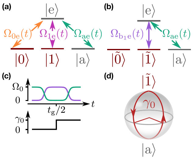 Figure 1
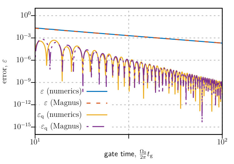 Figure 2
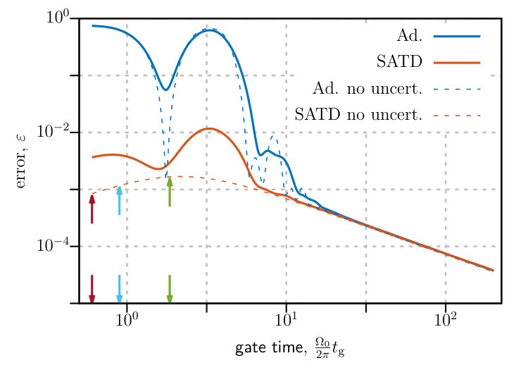 Figure 3
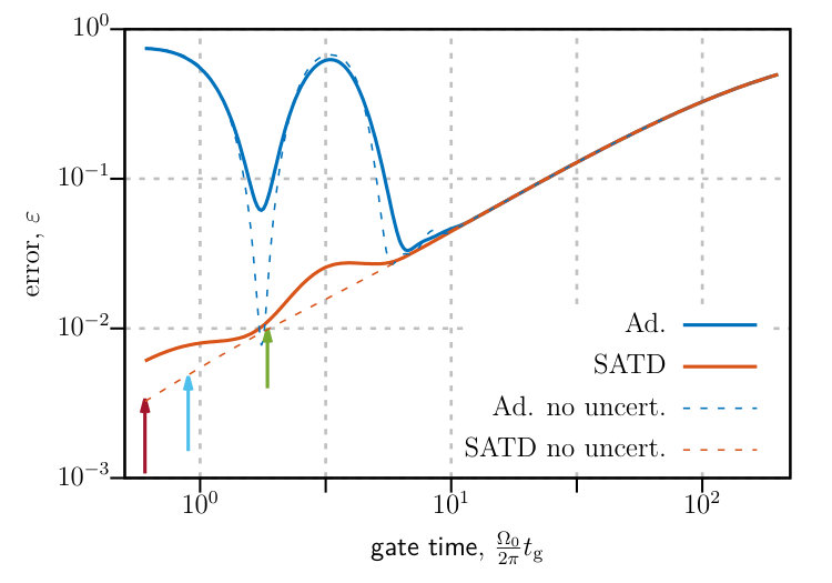 Figure 4
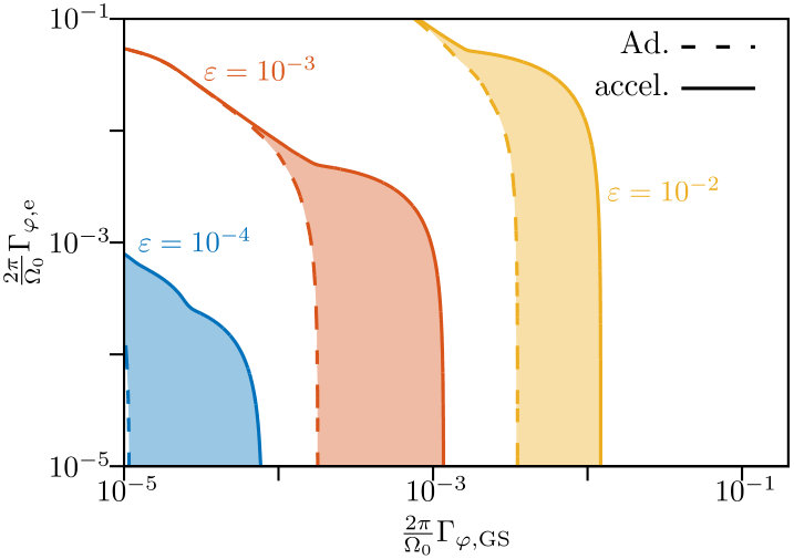 Figure 5
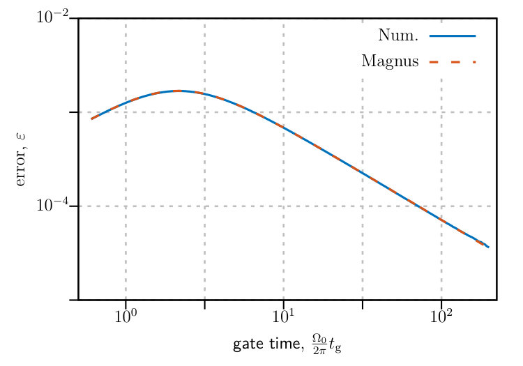 Figure 6
Peer Reviews
No public reviews on file for this paper yet. If you reviewed it on a platform where reviews are public (OpenReview, ICLR, NeurIPS, ICML), you can paste yours below so the community can read it here.
Videos
No videos yet. Explain this paper in a talk, walkthrough, or lecture? Add one.
Accelerated adiabatic quantum gates: optimizing speed versus robustness
Hugo Ribeiro
Max Planck Institute for the Science of Light, Staudtstraße 2, 91058 Erlangen, Germany
Aashish A. Clerk
Institute for Molecular Engineering, University of Chicago, 5640 South Ellis Avenue, Chicago, Illinois 60637, U.S.A.
Abstract
We develop new protocols for high-fidelity single qubit gates that exploit and extend theoretical ideas for accelerated adiabatic evolution. Our protocols are compatible with qubit architectures with highly isolated logical states, where traditional approaches are problematic; a prime example are superconducting fluxonium qubits. By using an accelerated adiabatic protocol we can enforce the desired adiabatic evolution while having gate times that are comparable to the inverse adiabatic energy gap (a scale that is ultimately set by the amount of power used in the control pulses). By modelling the effects of decoherence, we explore the tradeoff between speed and robustness that is inherent to shortcuts-to-adiabaticity approaches.
I Introduction
Any approach to implementing quantum gates requires applying time-dependent control fields to a system, such that the corresponding time-dependent Hamiltonian generates the desired unitary evolution. Regardless of the setting, ideal gates have two defining features: they are both robust against small imperfections in the amplitude, duration and phase of control pulses, and they are fast. Unfortunately, typical approaches to constructing gates optimize only one of these two desired characteristics. Schemes based on quantum adiabatic evolution (e.g. Duan et al. (2001); Kis and Renzoni (2002)) are typically extremely robust against parameter variations Møller et al. (2008), but suffer from extremely long protocol times. In contrast, more conventional non-adiabatic approaches can be extremely fast (approaching the quantum speed limit Mandelstam and Tamm (1991); Margolus and Levitin (1998); Deffner and Lutz (2013); Santos and Sarandy (2015); Pires et al. (2016); Marvian et al. (2016)), but require precise tuning of control pulses. In a typical experimental setting, neither approach is fully optimal, as both speed and robustness are important characteristics.
Given this, protocols that lie between these two extremes are highly desirable. This naturally leads one to the general approach of shortcuts to adiabaticity (STA) Demirplak and Rice (2003, 2005); Berry (2009); Ibáñez et al. (2012) (also known as counter-diabatic driving). STA are a family of techniques that allow one to mimic adiabatic evolution under some Hamiltonian using a modified Hamiltonian , in a much shorter timescale. STA protocols for evolving a well-defined initial state to some prescribed well-defined final state have been discussed in many contexts, and have even recently been implemented in a variety of experimental settings Bason et al. (2011); Schaff et al. (2011); Zhang et al. (2013); An et al. (2016); Du et al. (2016); Zhou et al. (2016); Kölbl et al. (2019). While not often stressed, STA protocols invariably involve a tuneable trade-off between speed and robustness. This tuneability can however be extremely useful in a real experimental setting, where the ultimate infidelity of a gate will be influenced by both these features. In Ref. Zhou et al. (2016), this tradeoff was discussed in the specific context of an accelerated STIRAP protocol implemented in an NV center system.
In this paper, we investigate the use of STA techniques to accelerate well-known adiabatic quantum gates based on a tripod level configuration, where three “ground state” levels all interact controllably with a single “excited state” level. Such schemes can find direct application in a variety of systems, including trapped ion qubits Duan et al. (2001); Srinivas et al. (2019) as well as superconducting qubits Manucharyan et al. (2009); Earnest et al. (2018). Accelerating a quantum gate is a more challenging problem than simply accelerating an adiabatic evolution with a single, well-defined initial state, as now one is interested in a manifold of possible initial states. In the case of a unique initial state, the (global) phase accumulated during the evolution is of no importance and it can consequently differ between the adiabatic and accelerated protocol. In stark contrast, when generating a quantum gate, the accumulated phases are of utmost importance. This is problematic, as standard STA techniques are not designed to preserve dynamical or geometric phases generated by adiabatic evolution. Despite this difference, we show that the superadiabatic transitionless driving (SATD) scheme developed in Ref. Baksic et al. (2016) to accelerate STIRAP-style quantum state transfer can be used to accelerate tripod-based adiabatic quantum gates. We also study in detail the tradeoffs entailed with using an accelerated protocol: while the protocol time can be dramatically reduced, one necessarily also becomes less tolerant of parameter variations, and also more sensitive to dissipative effects originating with the lossy excited level. The understanding we develop will allow one to design an optimally-constructed accelerated protocol for a given set of experimental parameters.
In contrast to other schemes Sjöqvist et al. (2012); Sjöqvist (2016); Abdumalikov Jr et al. (2013); Zhou et al. (2017) that generate non-adiabatic geometric gates, ours is purely geometric and does not rely on accumulating specific dynamical phases. This also distinguishes our work from the recent experiment by Yan et al. Yan et al. (2019), where an accelerated geometric gate is only obtained if a dynamical phase is cancelled by applying a -pulse. We also note that while Ref. Liu et al. (2017) straightforwardly applied the dressed state technique of Ref. Baksic et al. (2016) to accelerate an adiabatic gate, they did not consider the potential difficulties associated with this procedure (stemming from STA-induced modification of phases).
II Geometric Gates in a Tripod System
II.1 Basic double-STIRAP protocol
We start by reviewing how geometric qubit gates can be implemented in a four-level tripod system [see Fig. 1 (a)]. Our discussion complements existing literature Duan et al. (2001); Kis and Renzoni (2002) by providing a thorough discussion on how non-adiabatic errors deteriorate the performance of such gates. The system consists of three ground state levels (, , and ), each of which is controllably and resonantly coupled to a common excited state . The system Hamiltonian is
[TABLE]
where denotes the complex envelope of each control field.
We will use the ground states and to encode a logical qubit state. It allows one to use highly isolated states as qubit levels, thus potentially enabling long coherence times. This kind of situation can be realized in a variety of experimental platforms, e.g. in superconducting fluxonium qubits Manucharyan et al. (2009); Earnest et al. (2018).
We next parametrize the control fields, assuming only that they are chosen to keep the instantaneous eigenvalues of independent of time:
[TABLE]
determines the overall scale for the control fields [and the size of the energy gap of ], while the angles and determine their relative magnitudes. The angles and control the relative phases between control fields. For reasons that will become clear, we consider in what follows protocols where and are time-independent.
Diagonalizing the instantaneous Hamiltonian , one finds that it always possesses two zero-energy eigenstates that are orthogonal to . States in this “dark state” manifold are ideally suited for geometric gates, as they will never acquire dynamical phases. Further, there is always a unique dark state that is a superposition of qubit states only, namely
[TABLE]
This state does not depend on time. The orthogonal qubit-only state is
[TABLE]
and in general is not an instantaneous eigenstate of .
Writing in terms of these new qubit basis states yields
[TABLE]
where . We see that the qubit state is completely decoupled, whereas the qubit state forms a three-level -system Bergmann et al. (1998); Vitanov et al. (2017) with the states and [see Fig. 1 (b)]. One can now use well-known STIRAP protocols Bergmann et al. (1998); Vitanov et al. (2017) to adiabatically manipulate these states. In particular, using an appropriate double-STIRAP protocol we can engineer a cyclic evolution, such that the qubit state acquires a purely geometric Berry phase Pancharatnam (1956); Berry (1984). This will form the basis of our adiabatic single qubit gate (as first suggested in Refs. Duan et al. (2001); Kis and Renzoni (2002)).
To understand the double-STIRAP protocol, we first list the remaining instantaneous eigenstates of . In addition to the zero energy qubit dark state [c.f. Eq. (3)], in Eq. (5) also has a second, orthogonal zero energy dark state
[TABLE]
as well as two non-zero energy eigenstates:
[TABLE]
with instantaneous energies .
The double-STIRAP protocol involves adiabatically evolving the dark state from being purely at , to being at , and then back to being at the final time . This can be accomplished by choosing
[TABLE]
where is a monotonic function varying between and . The following form for is particularly effective:
[TABLE]
This choice gives a smooth turn on and turn off of the pulses, i.e. it satisfies . Note that at this stage, we do not specify the time-dependence of the relative phase ; as we will see, will determine the geometric phase acquired by . We assume for clarity that the control field is non-zero at . This is not restrictive. Even if one includes a finite turn-on time for this field, the additional resulting dynamics only effects the states (i.e. the auxiliary subspace. As shown in what follows, this does not hinder the realization of our geometric gate, as this gate is not contingent on any special preparation of the auxiliary subspace.
The system dynamics are best analyzed in the adiabatic frame. The frame-change operator is the time-dependent unitary that diagonalizes at each instant:
[TABLE]
In the adiabatic frame, we have
[TABLE]
where
[TABLE]
is a diagonal operator which generates the desired adiabatic evolution. In contrast, describes non-adiabatic errors in the evolution:
[TABLE]
Equation (13) differs from the non-adiabatic Hamiltonian derived in Ref. Baksic et al. (2016) because the latter work did not consider STIRAP with time-dependent relative phases.
If one now assumes that we are in the adiabatic limit, i.e. and , then we can ignore , and the unitary operator describing the evolution is
[TABLE]
where
[TABLE]
are the geometric phases accumulated by the dark and bright states, respectively.
Before proceeding, we note that there is an extremely simple choice for the relative control field phase that, despite first appearances, is compatible with adiabatic evolution. Namely, one can use
[TABLE]
where denotes the Heaviside step function. Despite the discontinuity at , there is no issue with adiabaticity. Note that our chosen pulse shapes [c.f. Eq. (2)] satisfy , implying that the phase is not well defined at this time; this allows the jump in Eq. (16). For a more geometric picture, note that this type of control results in a trajectory on the Bloch sphere that resembles a citrus wedge, as depicted in Fig. 1 (d). Finally we emphazise that this choice leads to [c.f. Eq. (15)].
We can express Eq. (14) in the (time-independent) lab frame via the transformation . Using for Eq. (16), we find at the final time
[TABLE]
Here, \hat{\mbox{\boldmath\sigma}}_{01}=(|0\rangle\!\langle 1|+\mathrm{H.c.},\,-i|0\rangle\!\langle 1|+\mathrm{H.c.},\,|0\rangle\!\langle 0|-|1\rangle\!\langle 1|) and \hat{\mbox{\boldmath\sigma}}_{\mathrm{a}\mathrm{e}}=(|\mathrm{a}\rangle\!\langle\mathrm{e}|+\mathrm{H.c.},\,-i|\mathrm{a}\rangle\!\langle\mathrm{e}|+\mathrm{H.c.},\,|\mathrm{a}\rangle\!\langle\mathrm{a}|-|\mathrm{e}\rangle\!\langle\mathrm{e}|) denote a vector of Pauli matrices. We have further defined the unit vectors
[TABLE]
and the rotation angle
[TABLE]
Equation (17) shows clearly that at the qubit subspace is decoupled from that of the two auxiliary levels. The evolution in the qubit subspace is a simple rotation. The rotation axis is controlled by the static pulse parameters , whereas the rotation angle is a geometric phase. We thus have a purely geometric arbitrary single qubit gate. We stress that having a gate that acts independently on the qubit and auxiliary subspaces is crucial: it allows a qubit gate to be performed without first having to prepare the state of the auxiliary levels.
II.2 Non-adiabatic errors
Our goal is to accelerate the adiabatic gate described above. As a first step, we need to understand the effects of non-adiabatic errors that occur when the protocol time is not infinitely slow compared to the inverse instantaneous energy gap of .
We can calculate non-adiabatic corrections to the evolution perturbatively in [c.f. Eq. (13)] using a Magnus expansion Magnus (1954). Using as defined in Eq. (8) with given by Eq. (9) and as defined in Eq. (16), we find to leading order (see Appendix A)
[TABLE]
with
[TABLE]
Comparing against Eqs. (17) and (20), we see that to leading order, non-adiabatic errors do not change the nature of the gate: we still have a pure geometric operation on the qubit subspace and the latter is still decoupled from the auxiliary subspace. Non-adiabatic errors only change the rotation performed on the auxiliary levels. The favourable scaling here is a direct consequence of our smooth choice for [c.f. Eq. (8)], whose derivatives vanish at the protocol start and end; this corresponds to the “boundary cancellation method” for non-adiabatic error suppression discussed in Refs. Lidar et al. (2009); Rezakhani et al. (2010); Wiebe and Babcock (2012).
A more useful measure for quantifying the impact of non-adiabatic errors is given by the state-averaged fidelity of the gate Pedersen et al. (2007)
[TABLE]
where denotes the trace operation, is the dimension of the Hilbert space, and where is given in Eq. (17) and is the unitary operator generated by Eq. (1) evaluated at . Using the approximate given in Eq. (20), we find
[TABLE]
However, it is misleading to compare to to determine the gating time for which the error goes above a critical threshold, e.g. for quantum error correction. In Eq. (23) the deviations from unity are only due to imperfect dynamics in the auxiliary subspace as we identified earlier on [see Eqs. (17) and (20)]. Since Eq. (22) holds for any linear operator in a -dimensional Hilbert space, we consider instead that allows us to quantify errors that only affect the dynamics in the qubit subspace. Here, is the projector onto the qubit subspace. corresponds to measuring the overlap between the unitary operator and the operator ; the latter is not necessarily unitary. Due to the direct sum structure of [cf. (17)], the projection operation yields the ideal gate acting on the qubit subspace only.
Within this framework, and performing a fourth order Magnus expansion (see Appendix A), we find
[TABLE]
with . We stress that there exists special gate times for which the fidelity is equal to unity. Using Eq. (24), we find those times to be
[TABLE]
This phenomenon (a coherent cancellation of non-adiabatic effects) has also been discussed in Ref. Wiebe and Babcock (2012).
In Fig. 2, we plot the error [see Eq. (22)] as a function of gate time for and both obtained numerically by integrating the Schrödinger equation and perturbatively via the Magnus expansion. In the adiabatic regime, i.e. , the Magnus expansion fully captures deviations from the ideal adiabatic evolution which confirms our error scaling analysis. However, even with the improved error scaling in the qubit subspace, the achievable gate times in a realistic setup remain longer than typical decoherence rates.
III Accelerated Gate
We now turn to the main goal of this paper: how can we accelerate the geometric qubit gate presented in Sec. II.1 using the general philosophy of “shortcuts to adiabaticity” (STA) Demirplak and Rice (2003, 2005, 2008); Berry (2009); Baksic et al. (2016)? At first glance, this is a non-trivial problem. The purpose of STAs is to accelerate the evolution of a specific initial state, and usually, one does not care about the final, overall phase of the state. In contrast, we want to accelerate the evolution of an arbitrary initial qubit state, and the phases acquired by the adiabatic states are of crucial importance. Despite these difficulties, we show that our desired goal can indeed be accomplished. We will use our recently proposed dressed-state approach, which allows acceleration of STIRAP-type processes by simply modifying the form of the original control pulses Baksic et al. (2016); Zhou et al. (2016). Note that Ref. Liu et al. (2017) did not consider these difficulties; as we show below, it is not a trivial task to find a suitable STA that preserves the phases acquired by the adiabatic states.
Our goal will be to modify the three control fields () from the values given in Eqs. (2) and (8), so that the desired gate operation is accomplished even though the total protocol time is not long compared to . This modification can be described by adding a term to the Hamiltonian, i.e. . In the adiabatic frame, this modification can be written as
[TABLE]
One can readily verify that transforming Eq. (26) to the original frame, , results in a control Hamiltonian having the same form as Eq. (1); no additional control fields are required. Note that the qubit-only dark state remains decoupled for any choice of the , .
Conventional STAs attempt to modify so that the evolution follows the (original) adiabatic trajectory at all times. In contrast, the dressed-state approach of Ref. Baksic et al. (2016) aims for something less extreme. We let the system deviate from the adiabatic trajectory at intermediate times. This can be framed as a time-dependent dressing of the original adiabatic eigenstate, with the dressing vanishing at and . For our problem, we need to add an additional constraint. We must find a dressed version of the dark state
[TABLE]
which retains the geometric nature of the evolution. In other words we require that the new dressed dark state does not acquire any dynamical phases.
III.1 Generic dressing
Following Ref. Baksic et al. (2016) we try a simple dressing transformation
[TABLE]
where the dressing angle remains to be determined. It must satisfy , to ensure the dressing vanishes at the start and end of the protocol (which then guarantees at and ). Note that at this stage we only assume to be of the form given in Eq. (8) while no particular form is assumed for .
The goal is now to pick the dressing parameter and control modifications such that the resulting dynamics does not cause transitions out of the dressed dark state. By considering the dynamics in the time-dependent frame defined by Eq. (28) (dressing frame), we find that this can be accomplished by choosing the dressing angle to fulfill the differential equation
[TABLE]
and the control fields to be
[TABLE]
Unfortunately, suppressing unwanted transitions is not enough to achieve our gate. We also need control over the phase acquired by the dressed dark state. In particular, it should not acquire a dynamical phase which depends explicitly on while still accumulating a geometrical phase. We stress that the control fields in Eq. (30) also cancel the purely dynamical phase originating from the dressing by ensuring that the energy of the dressed dark state is [math]. Within this framework the phase accumulated by the dressed dark state is given by
[TABLE]
In spite of the similarities with Eq. (15), there is no guarantee that this phase is purely geometric since one might not be able to express as a function of and only. In our example, however, the situation is far worse. A solution of Eq. (29) that fulfills the requirement that the dressing must vanish at the boundaries, [] leads to to be an antisymmetric function on the interval since is symmetric on said interval [see Eq. (8)]. Using the symmetry of the functions involved in Eq. (31), one finds .
III.2 Spin-based dressing
However, for given by Eq. (16) and arbitrary of the form in Eq. (8), one can find a large class of STAs for which there is an accumulated phase whose nature is geometric. To proceed, we first define effective spin- operators to describe the dressed frame states: , , and . The dressing transformation of interest is then:
[TABLE]
In the dressed frame, the Hamiltonian is given by
[TABLE]
with
[TABLE]
[TABLE]
and
[TABLE]
We have written Eq. (33) as the sum of a spin Hamiltonian [see Eq. (34)], a non-spin Hamiltonian [see Eq. (35)], and a Hamiltonian that generates the geometric phase [see Eq. (36)]. We also defined the effective magnetic field components
[TABLE]
as well as the parameters of the non-spin Hamiltonian:
[TABLE]
The choice of dressing in Eq. (32) was made to ensure that ; this partly solves the problem of the STA giving rise to unwanted dynamical phases in the evolution of the dressed dark state . In contrast to the STA approach (see Sec. III.1), we do not start by looking for a dressing angle that generates a dressing transformation that cancels unwanted transitions (between dressed dark state and dressed bright states). Instead, we start by looking for a that gives a specific value for the phase accumulated by the dressed dark state . Neglecting for a moment transitions involving the dressed dark state, we have that the phase accumulated by is given by
[TABLE]
Taking into account that we have chosen a particular form for [see Eq. (16)] and comparing Eq. (39) to Eq. (15), we see that the phase accumulated by the dressed dark state is equal to the adiabatic-limit dark state geometric phase if
[TABLE]
i.e. we must restrict ourselves to a class of dressing transformations that exactly vanish halfway through the protocol.
There is a second consequence of having to work with dressing transformations that fulfill Eq. (40): one can easily verify that does not generate any dynamics. Since , integrating between and yields because we evaluate at where and such that all parameters defined in Eq. (38) evaluate to [math].
Within this framework all that remains is to find a specific dressing function satisfying Eq. (40), and a corresponding control Hamiltonian that cancels unwanted transitions generated by . This is essentially equivalent to the general problem treated in Ref. Baksic et al. (2016). While many choices are possible, a particular simple approach is the so-called superadiabatic transitionless driving (SATD) dressing introduced in Ref. Baksic et al. (2016). This is defined by the specific dressing angle
[TABLE]
This satisfies our constraint Eq. (40) as long as the initial pulse sequence satisfies . For example, the pulse shape in Eq. (9) satisfies this property.
Before proceeding we note that the phase accumulated by the dressed dark state can still be viewed as a geometric phase. As long as Eq. (40) is fulfilled the accumulated phase is independent of the protocol time and does not depend on the details of the pulse. We stress, however, one more time that the dressing transformation allowing one to get a STA that preserves the geometric nature of the phase accumulated by the dressed dark state explicitly depends on our choice of and that our specific choice of dressing [see Eq. (41)] further requires the adiabatic protocol to obey .
For this choice of dressing, the required modified control fields (which cancel transitions out of the dressed dark state) are:
[TABLE]
Combining these results, we find that the accelerated dynamics results in an evolution that at yields the gate
[TABLE]
whose action on the qubit subspace is the same as [see Eq. (17)], but acts differently on the auxiliary subspace. The latter undergoes a rotation of angle around the axis
[TABLE]
with .
We note that Eq. (43) always leads to a perfect qubit-subspace fidelity independent of the speed of the protocol.
IV Dissipative Dynamics
In the following section, we characterize the performance of both the adiabatic and STA gates in the presence of imperfections. We consider two types of imperfections: dissipation and uncertainties in the parameters of the Hamiltonian.
To model the loss we consider a Lindblad master equation that describes pure dephasing of the ground and excited states
[TABLE]
where is the Hamiltonian, is the density operator of the system, () is the dephasing rate of state , and we have defined the anti-commutator . We stress that in the adiabatic frame the dephasing processes we are considering lead to transitions between instantaneous eigenstates. For this reason we do not explicitly consider relaxation processes.
To quantify how decoherence affects the performance of the gate, we use the result of Bowdrey et al. for the average fidelity of single qubit maps Bowdrey et al. (2002)
[TABLE]
where with is an axial pure state on the Bloch sphere of the qubit, e.g. , was defined earlier in the text, and is a solution of Eq. (45) for the initial state .
In addition to errors due to noise, we also consider errors arising from uncertainties in the system Hamiltonian. Here, we assume that the amplitude parameter [cf. Eqs. (1) and Eq. (2)] is only known with finite precision, as described by a probability distribution . In the following we assume to be uniform on the interval with . The performance of the gate is then quantified via the averaged average fidelity
[TABLE]
For the results that follow, accelerated gates are implemented using a starting pulse shape given by Eq. (9) and the SATD STA defined by Eqs. (41) and (42).
IV.1 Excited State Dephasing
In Fig. 3, we plot the error as a function of the gate time for , , , , and for for both the adiabatic (blue traces) and accelerated protocol (orange traces) either without uncertainty on (dashed traces) or with an uncertainty of () on (solid traces). We have indicated with a green arrow the shortest gate time for which the maximal amplitude of the modified controls is still , with a blue (red) arrow the gate time for which the energy cost to generate the STA is twice (three times) as large as the energy cost to generate the adiabatic control sequence. We define the energy cost of a control sequence as
[TABLE]
where is the operator norm equal to the largest singular value of the Hamiltonian operator denoted by .
We start by observing that going to the adiabatic regime, , results in both gates becoming insensitive to noise and uncertainty. This is expected because the evolution of the system can be reduced to the evolution of the dark state [see Eq. (6)] which contains no excited state amplitude. We note that for the accelerated gate, going to the adiabatic regime results in a vanishing dressing such that the dressed dark state is effectively . Moreover, a small uncertainty on the instantaneous gap is irrelevant as long as . It is only outside of the adiabatic regime that both gates are affected by a lossy excited state since during the evolution the excited state will be occupied. One clearly sees that the accelerated version of the gate outperforms its adiabatic counterpart; this reflects the fact that the mechanism leading to excited state occupancy is different in each case.
For the adiabatic version of the gate, non-adiabatic processes are responsible for the transitions between the dark state and the bright states , which contain a finite excited state amplitude [see Eq. (7)]. Since non-adiabatic transitions need first to happen for noise in the excited state to disrupt the dynamics, the gate error is mainly dominated by non-adiabatic errors. However, signatures of the dissipative dynamics can be observed for the special times [see Eq. (25)] for which the coherent evolution brings the system back to the dark state. These special times do not lead to a perfect gate anymore because the coherent mechanism that brings the system back to the dark state is disrupted by excited state dephasing. This coherent mechanism is further hindered by the uncertainty on .
The accelerated gate is constructed such that whatever amplitude leaves the dark state it has to come back to the dark state by the end of the protocol; this is equivalent to having the system remaining in the dressed dark state for the whole evolution. However, leaving the dark state is not harmless in the presence of a noisy excited state: it disrupts the STA dynamics in two ways. First, there is no guarantee that the amplitude leaving the dark state comes back by the end of the evolution. Second, even if the amplitude that left the dark state comes back, it could come back with a phase error. These two mechanism can be identified as the leading order processes leading to deviations of the average fidelity [Eq. (46)] from unity. Using a Magnus expansion we can find approximate solutions of Eq. (45) which we use to evaluate [Eq. (46)] (see Appendix B). We find
[TABLE]
which is in good agreement with numerical simulations [see Appendix B]. In particular, Eq. (49) captures the non-monotonic behavior of the gate error as a function of gate time. Sufficiently faster gates become insensitive to a lossy excited state. We note, however, that reaching such a regime experimentally is difficult.
In the presence of uncertainty in , it is impossible to realize the exact STA that would cancel out non-adiabatic transitions. As a result, a small non-adiabatic transition probability from the dressed dark state to the bright states remains. This becomes apparent for faster gate times where the fidelity of the accelerated gates oscillates in sync with the fidelity of the adiabatic gate.
Finally, we note that in this scenario if being fast is not essential, then there is no benefit in using an accelerated gate. Both gates perform equally well in the adiabatic regime. However, if the gate time has to be below a threshold outside of the adiabatic regime, then the accelerated gate will outperformed the adiabatic one.
IV.2 Ground and Excited State Dephasing
In Fig. 4, we plot the error, , as a function of the gate time for , , , , and for both the adiabatic (blue traces) and accelerated protocol (orange traces) either without uncertainty on (dashed traces) or with an uncertainty of () on (solid traces). Similarly to Fig. 3, we have indicated with a green arrow the shortest gate time for which the maximal amplitude of the modified controls is still , with a blue (red) arrow the gate time for which the energy cost [see Eq. (48)] to generate the STA is twice (three times) as large as the energy cost to generate the adiabatic control sequence.
In contrast to the case where only the excited state is lossy, operating in the adiabatic regime does not lead to a perfect gate. The dephasing on the ground state manifold sets a threshold for the slowest “allowed” gate time. As a consequence, the adiabatic version of the gate becomes an unviable option. Trying to perform the gate faster to avoid ground state dephasing unavoidably leads to a regime where the dominating source of errors are non-adiabatic transitions. On the other hand, the accelerated gate is less susceptible to non-adiabatic errors. As a result decreasing the gate time allows one to escape the interval for which the error is mainly dominated by ground state dephasing, , to operate in a regime where only excited state dephasing contributes to the gate error.
In this scenario, being fast becomes essential and corresponds to a situation where the accelerated gate provides a real benefit over its adiabatic counterpart.
IV.3 Extended Robustness Comparison
To identify the regimes where the accelerated gate provides a clear benefit over the adiabatic gate, we look for the gate time that yields the smallest error for fixed dephasing rates. We have constrained the minimal gate time by imposing that the maximal amplitude of the modified pulse sequence cannot be larger than . For simplicity we consider the case where the ground state dephasing rates are equal, i.e. . We also assume that the uncertainty on is (). In Fig. 5, we plot contour lines for different error thresholds as a function of and for the adiabatic gate (dashed lines) and accelerated gate (solid lines). For the displayed contours, we see that the accelerated gate reaches the same error level as the adiabatic gate for rates that can be roughly up to one order of magnitude larger.
V Conclusion
We have shown how to use the framework of shortcuts-to-adiabaticity to accelerate geometric gates in tripod systems. We have discussed both how standard STA techniques designed for the transfer of a single known state are problematic due to STA-induced modification of dynamical and geometric phases. We have also shown a set of protocols that overcome this seeming limitation and discussed the advantages of using accelerated gates in the presence of dissipation and Hamiltonian uncertainties: the accelerated gate preserves the robustness against parameter variations and allows one to be fast enough to overcome thresholds set by relaxation and dephasing times. Our accelerate control scheme can be implemented in a variety of state-of-the-art qubit implementations.
Our work also suggests that accelerated geometric-based two-qubit gates could be developed for a variety of systems. In particular, it could greatly benefit superconducting-based architectures where two-qubit gates are still the main limitation preventing the realization of high-fidelity complex gate sequences.
VI Acknowledgements
This work was supported by the Army Research Office under Grant No. W911NF-19-1-0328.
Appendix A Average Gate Fidelity with Unitary Evolution
In this appendix we show how to use a Magnus expansion to obtain approximate solutions of the Schrödinger equation
[TABLE]
where was defined in Eq. (5) of the main text. We focus on the special case where the control field phase is given by Eq. (16). The special form of and the symmetry of the function [see Eq. (8)] allows us to split the evolution into two distinct STIRAP processes defined by the Hamiltonians
[TABLE]
which describes the first half of the evolution that brings the system from to , and
[TABLE]
which describes the second half of the evolution that brings back to . Here, [see Eq. (9)] is defined for and we have used the symmetry of the function [see Eq. (8)] to obtain Eq. (52). Within this framework the evolution operator can be parametrized as
[TABLE]
where is generated by [see Eq. (51)] and is generated by [see Eq. (52)]. We stress that is continuous at because the actual coupling strength between and is 0, which allows us in the first place to have a phase jump.
It is useful to look for solutions of Eq. (50) in the adiabatic frame. We can transform Eqs. (51) and (52) to the adiabatic frame by using the frame-change operator defined in Eq. (10) of the main text with
[TABLE]
and
[TABLE]
We find
[TABLE]
where () denotes [] in the adiabatic frame. We have introduced the spin operators and . We note that the remaining spin operator was introduced in the main text below Eq. (32). It is convenient to transform Eq. (56) to the interaction picture generated by to perform the Magnus expansion, this yields
[TABLE]
It is useful to notice that the dynamics generated by can be parametrized as
[TABLE]
with , , , and . This form allows us to get an exact representation for by expanding the exponential into a series and using the properties of the spin operators. The functions , , and are found perturbatively using a fourth-order Magnus expansion Magnus (1954). We find that at these functions evaluate to
[TABLE]
with , , , , , and .
Finally, the evolution operators are given by
[TABLE]
with .
We can evaluate Eq. (22) with [see text below Eq. (23)] and [see Eq. (53)] (not shown due to the length of the result). To get Eq. (24), one further needs to expand the trigonometric functions involved in the result to fourth-order in and collect terms up to sixth-order in .
Appendix B Average Map Fidelity with Excited State Dephasing
In this section we present the general framework allowing us to evaluate perturbatively the average fidelity of the qubit map [cf. Eq. (46)] for the accelerated gate in the presence of excited state dephasing. We start by defining the modified Hamiltonian with the SATD correction
[TABLE]
where is the Hamiltonian of the tripod system written in terms of the new qubit states [cf. Eq. (5)] and
[TABLE]
In the frame defined by the SATD dressing [see Eqs. (32) and (41)], the master equation describing the evolution of the tripod system with excited dephasing is given by
[TABLE]
with and .
Using a superoperator formalism Eq. (63) can be written as
[TABLE]
where and and we have defined with . We also introduced the complex conjugation and transpose operation denoted by and , respectively.
To find approximate solutions of Eq. (64) it is convenient to work in the interaction picture defined by . In this frame Eq. (64) reduces to
[TABLE]
where and is the solution of , i.e. . Within this framework the solution of Eq. (64) is given by where is a solution of Eq. (65). Using a first order Magnus expansion Magnus (1954), we can approximate by
[TABLE]
This leads to an approximate solution for ,
[TABLE]
which can be used to evaluate Eq. (46).
In Fig. 6 we plot the error as a function of gate time for , , , and for the accelerated protocol calculated numerically (solid blue trace) and using Eq. (49) (dashed orange trace). As stated in the main text, the approximate analytical result is in very good agreement with the numerical results.
The reference list from the paper itself. Each links out to its DOI / PubMed record.
- 1Duan et al. (2001) L.-M. Duan, J. I. Cirac, and P. Zoller, Geometric manipulation of trapped ions for quantum computation, Science 292 , 1695 (2001) . · doi ↗
- 2Kis and Renzoni (2002) Z. Kis and F. Renzoni, Qubit rotation by stimulated raman adiabatic passage, Phys. Rev. A 65 , 032318 (2002) . · doi ↗
- 3Møller et al. (2008) D. Møller, L. B. Madsen, and K. Mølmer, Geometric phases in open tripod systems, Phys. Rev. A 77 , 022306 (2008) . · doi ↗
- 4Mandelstam and Tamm (1991) L. Mandelstam and I. Tamm, The uncertainty relation between energy and time in non-relativistic quantum mechanics, in Selected Papers , edited by B. M. Bolotovskii, V. Y. Frenkel, and R. Peierls (Springer Berlin Heidelberg, Berlin, Heidelberg, 1991) pp. 115–123. · doi ↗
- 5Margolus and Levitin (1998) N. Margolus and L. B. Levitin, The maximum speed of dynamical evolution, Physica D: Nonlinear Phenomena 120 , 188 (1998) . · doi ↗
- 6Deffner and Lutz (2013) S. Deffner and E. Lutz, Quantum speed limit for non-markovian dynamics, Phys. Rev. Lett. 111 , 010402 (2013) . · doi ↗
- 7Santos and Sarandy (2015) A. C. Santos and M. S. Sarandy, Superadiabatic controlled evolutions and universal quantum computation, Scientific Reports 5 , 15775 (2015) . · doi ↗
- 8Pires et al. (2016) D. P. Pires, M. Cianciaruso, L. C. Céleri, G. Adesso, and D. O. Soares-Pinto, Generalized geometric quantum speed limits, Phys. Rev. X 6 , 021031 (2016) . · doi ↗