The SDP value for random two-eigenvalue CSPs
Sidhanth Mohanty, Ryan O'Donnell, Pedro Paredes

TL;DR
This paper precisely determines the SDP (quantum) value of large random two-eigenvalue CSPs, extending previous results and introducing new techniques that may indicate a computational threshold.
Contribution
It extends the analysis of SDP values to new classes of random CSPs using advanced spectral and nonbacktracking operator techniques.
Findings
SDP value matches spectral relaxation in large random instances
Includes new cases like random Sort4 and Forrelation CSPs
Techniques generalize nonbacktracking operators and Ihara--Bass Formula
Abstract
We precisely determine the SDP value (equivalently, quantum value) of large random instances of certain kinds of constraint satisfaction problems, ``two-eigenvalue 2CSPs''. We show this SDP value coincides with the spectral relaxation value, possibly indicating a computational threshold. Our analysis extends the previously resolved cases of random regular and , and includes new cases such as random (equivalently, ) and CSPs. Our techniques include new generalizations of the nonbacktracking operator, the Ihara--Bass Formula, and the Friedman/Bordenave proof of Alon's Conjecture.
Click any figure to enlarge with its caption.
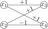 Figure 1
 Figure 2
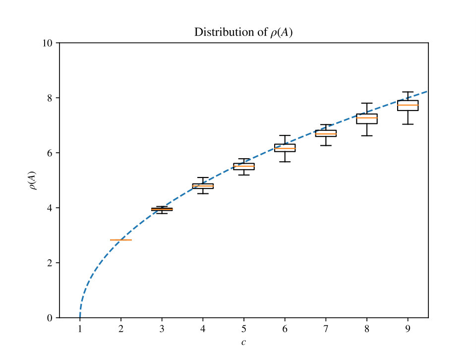 Figure 3
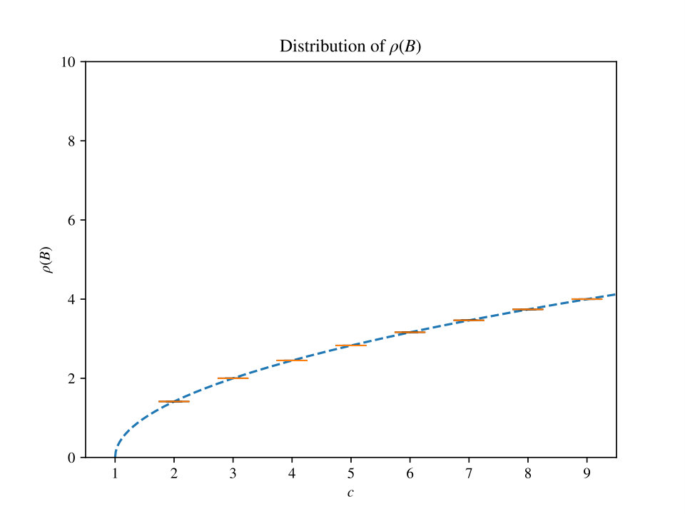 Figure 4
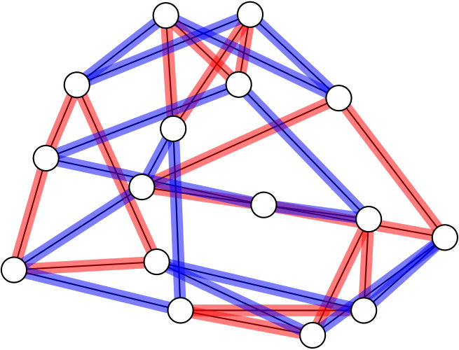 Figure 5
 Figure 6
 Figure 7
 Figure 8
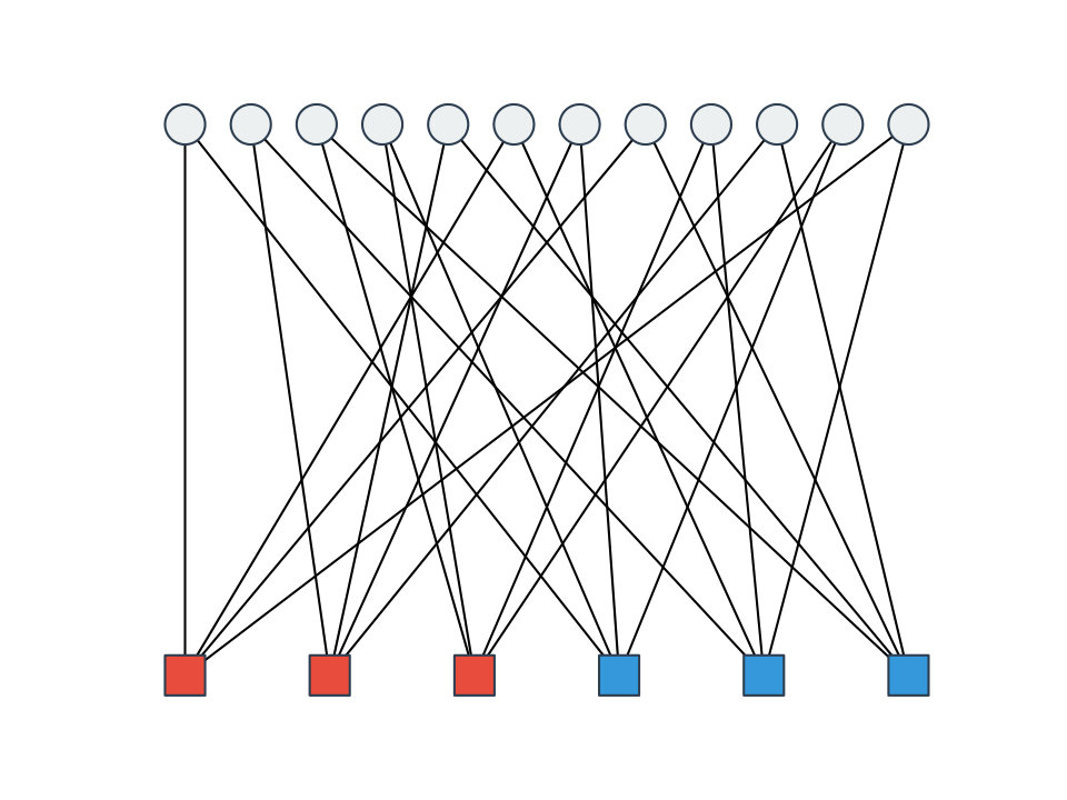 Figure 9
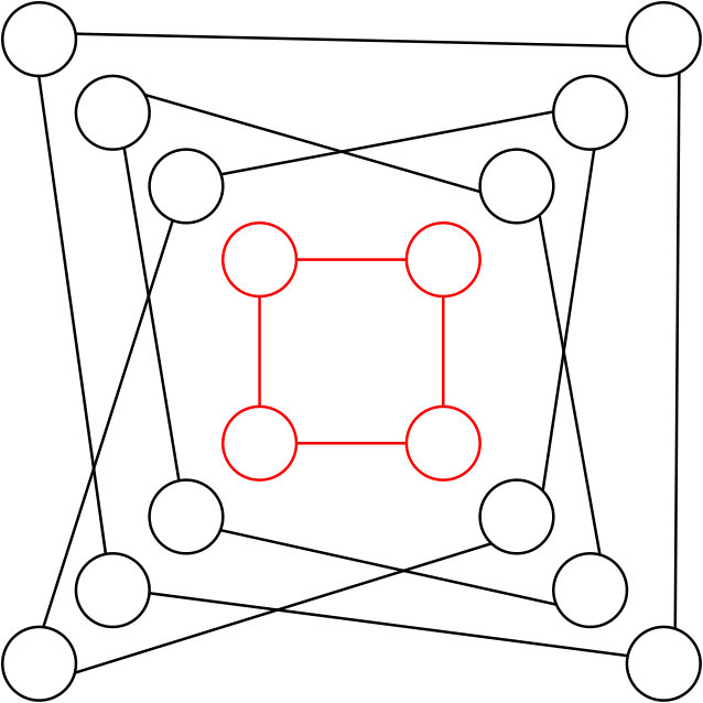 Figure 10
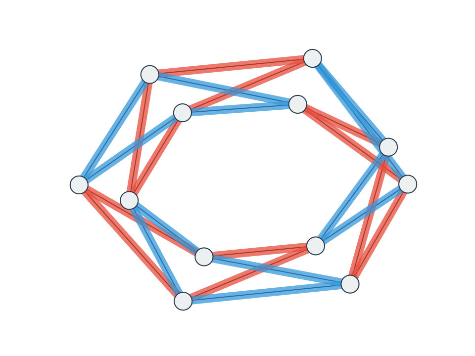 Figure 11
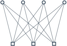 Figure 12
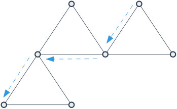 Figure 13
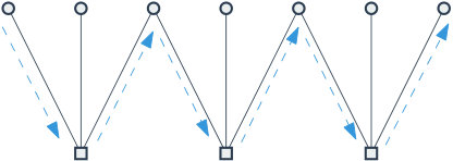 Figure 14
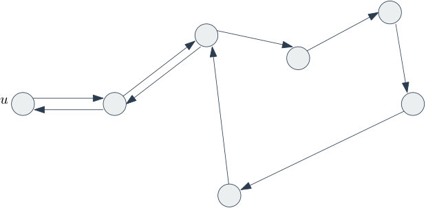 Figure 15
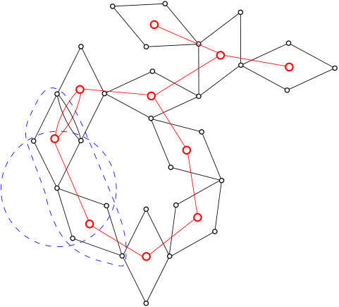 Figure 16
 Figure 17
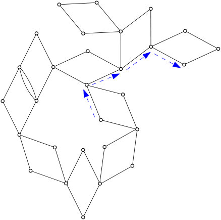 Figure 18
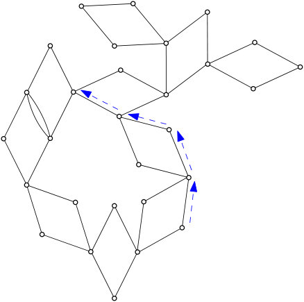 Figure 19
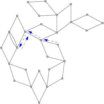 Figure 20
 Figure 21
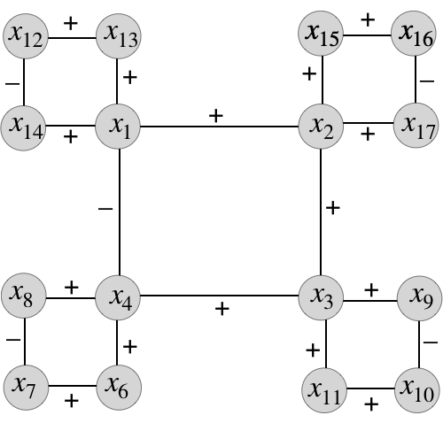 Figure 22
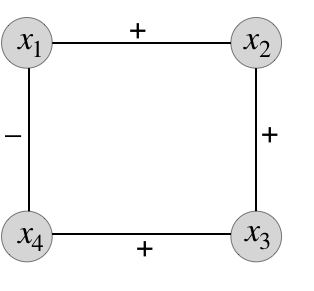 Figure 23
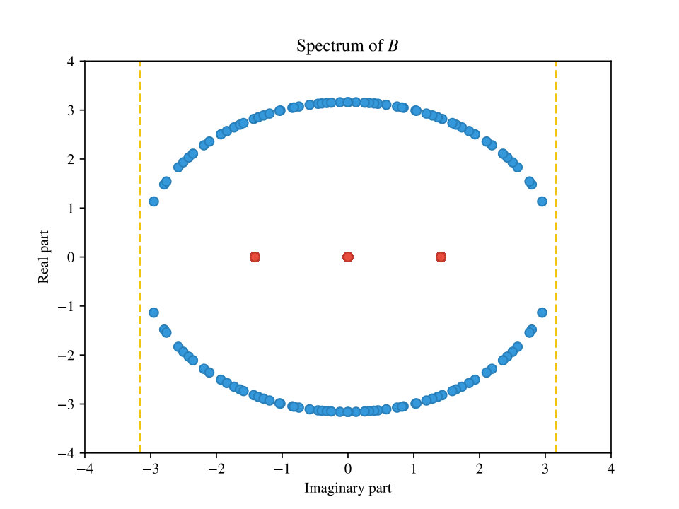 Figure 24
 Figure 25
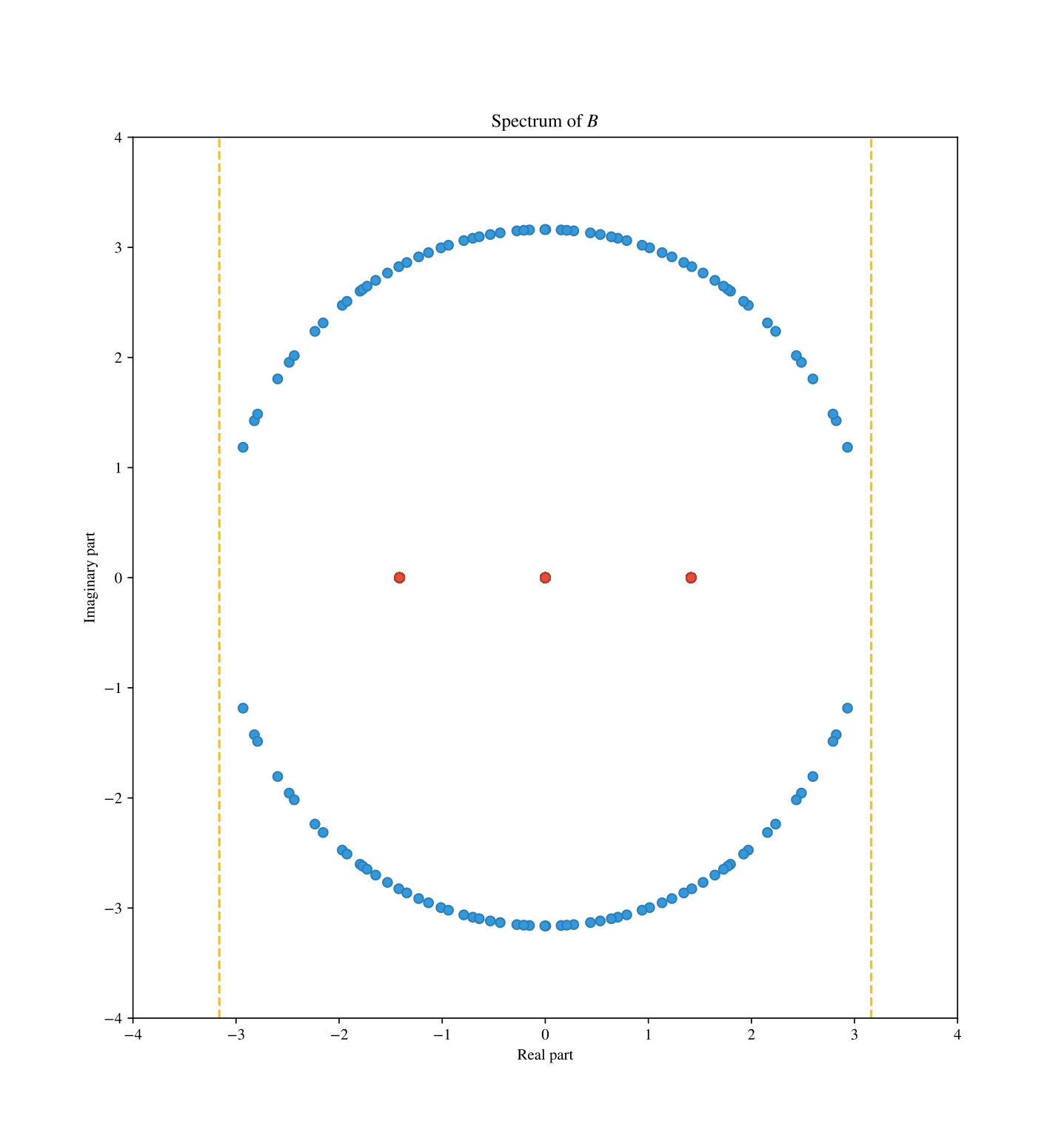 Figure 26
Peer Reviews
No public reviews on file for this paper yet. If you reviewed it on a platform where reviews are public (OpenReview, ICLR, NeurIPS, ICML), you can paste yours below so the community can read it here.
Videos
No videos yet. Explain this paper in a talk, walkthrough, or lecture? Add one.
The SDP value for random two-eigenvalue CSPs
Sidhanth Mohanty EECS Department, University of California Berkeley. Supported by NSF grant CCF-1718695
Ryan O’Donnell Computer Science Department, Carnegie Mellon University. Supported by NSF grant CCF-1717606. This material is based upon work supported by the National Science Foundation under grant numbers listed above. Any opinions, findings and conclusions or recommendations expressed in this material are those of the author and do not necessarily reflect the views of the National Science Foundation (NSF).
Pedro Paredes
Abstract
We precisely determine the SDP value (equivalently, quantum value) of large random instances of certain kinds of constraint satisfaction problems, “two-eigenvalue 2CSPs”. We show this SDP value coincides with the spectral relaxation value, possibly indicating a computational threshold. Our analysis extends the previously resolved cases of random regular and , and includes new cases such as random (equivalently, ) and CSPs. Our techniques include new generalizations of the nonbacktracking operator, the Ihara–Bass Formula, and the Friedman/Bordenave proof of Alon’s Conjecture.
Contents
-
1.2.1 Friedman/Bordenave Theorems for two-eigenvalue additive lifts
-
2.4 Random constraint graphs, instance graphs, and additive products
-
3 An Ihara–Bass formula for additive lifts of 2-eigenvalue atoms
-
6.3 Tangle-free, singleton-free linkages are nearly duplicative
1 Introduction
This work is concerned with the average-case complexity of constraint satisfaction problems (CSPs). In the theory of algorithms and complexity, the most difficult instances of a given CSP are arguably random (sparse) instances. Indeed, the assumed intractability of random CSPs underlies various cryptographic proposals for one-way functions [Gol00, JP00], pseudorandom generators [BFKL93], public key encryption [ABW10], and indistinguishability obfuscation [Lin17], as well as hardness results for learning [DS16] and optimization [Fei02]. Random CSPs also provide a rich testbed for algorithmic and lower-bound techniques based on statistical physics [MM09] and convex relaxation hierarchies [KMOW17, RRS17].
For a random, say, instance average degree , its optimum value is with high probability (whp) concentrated around a certain function of . Similarly, given a random instance where each variable participates in an average of clauses, the satisfiability status is whp determined by . However explicitly working out the optimum/satisfiability as a function of is usually enormously difficult; see, for example, Ding–Sly–Sun’s landmark verification [DSS15] of the threshold for sufficiently large , or Talagrand’s proof [Tal06] of the Parisi formula for the Sherrington–Kirkpatrick model ( with random Gaussian edge weights). The latter was consequently used by Dembo–Montanari–Sen [DMS17] (see also [Sen18]) to determine that the value in a random -regular graph is a fraction of edges (whp), where is an analytic constant arising from Parisi’s formula.
Computational gaps for certification.
Turning to computational issues, there are two main algorithmic tasks associated with an -variable CSP: searching for an assignment achieving large value (hopefully near to the optimum), and certifying (as, e.g., convex relaxations do) that no assignment achieves some larger value. Let’s take again the example of random -regular , where whp we have . It follows from [Lyo17] there is an efficient algorithm that whp finds a cut of value at least . One might say that this provides a -approximation for the search problem,111Depending on one’s taste in normalization; i.e., whether one prefers the objective function or , for . where . On the other side, the in a -regular graph is always at most , and Friedman’s proof of Alon’s Conjecture [Fri08] shows that whp; thus computing the smallest eigenvalue efficiently certifies . One might say that this efficient spectral algorithm provides a -approximation for the certification problem, where .
It is a very interesting question whether either of these approximation algorithms can be improved. On one hand, it would seem desirable to have efficient algorithms that come arbitrarily close to matching the “true” answer on random inputs. On the other hand, the nonexistence of such algorithms would be useful for cryptography and hardness-of-approximation and -learning results.
Speaking broadly, efficient algorithms for the search problem seem to do better than efficient algorithms for the certification problem. For example, given a random instance with clause density slightly below the satisfiability threshold of , there are algorithms [MPR16] that seem to efficiently find satisfying assignments whp. On the other hand, the longstanding Feige Hypothesis [Fei02] is that efficient algorithms cannot certify unsatisfiability at any large constant clause density, and indeed there is no efficient algorithm that is known to work at density . Similarly, for the Sherrington–Kirkpatrick model, Montanari [Mon18] has recently given an efficient PTAS for the search problem222Modulo a widely believed analytic assumption., whereas the best known efficient algorithm for the certification problem is again only a -approximation. These kinds of gaps seem to be closely related to “information-computation gaps” and Kesten–Stigum thresholds for information recovery and planted-CSP problems.
In this work we focus on potential computational thresholds for random CSP certification/refutation problems in the sparse setting, and in particular how these thresholds depend on the “type” of the CSP. For CSPs with a predicate supporting a pairwise-uniform distribution — such as or , — there is solid evidence that the computational threshold for efficient certification of unsatisfiability is very far from the actual unsatisfiability threshold. Such CSPs are whp unsatisfiable at constant constraint density, but any polynomial-time algorithm using the powerful Sum-of-Squares (SoS) algorithm fails to refute unless the density is [KMOW17]. But outside the pairwise-supporting case, and especially for “-like” CSPs such as and (Not-All-Equal ), the situation is much more subtle. For one, the potential gaps are much more narrow; e.g., in random , even a simple spectral algorithm efficiently refutes satisfiability at constant constraint density. Thus one must look into the actual constants to determine if there may be an “information-computation” gap. Another concern is that evidence for computational hardness in the form of SoS lower bounds (degree or higher) seems very hard to come by (see, e.g., [Mon17]).
Prior work.
Let us describe two prior efforts towards computational thresholds for upper-bound-certification in “-like” random CSPs. Montanari and Sen [MS16] (see also [BKM17]) investigated the problem in random -regular graphs, where the optimum value is whp (ignoring factors). Friedman’s Theorem implies that the basic eigenvalue bound efficiently certifies the value is at most . By using a variant of the Gaussian Wave [Elo09, CGHV15, HV15] construction for the infinite -ary tree, Montanari and Sen were able to show that even the Goemans–Williamson semidefinite programming (SDP) relaxation [DP93, GW95] is still just whp. This may be considered evidence that no polynomial-time algorithm can certify upper bounds better than , as Goemans–Williamson has seemed to be the optimal polynomial-time algorithm in all previous circumstances. Of course it would be more satisfactory to see higher-degree SoS lower bounds, but as mentioned these seem very difficult to come by.
Recently, Deshpande et al. [DMO*+*19] have given similar results for random “-constraint-regular” CSPs; i.e., random instances where each variable participates in exactly constraints.333We have changed terminology to avoid a potential future confusion; we will be associating constraints with triangle graphs, so -constraint-regular instances will be associated to -regular graphs. Random -constraint-regular instances of are easily shown to be unsatisfiable (whp) for . Deshpande et al. identified an exact threshold result for when the natural SDP algorithm is able to certify unsatisfiability: it succeeds (whp) if and fails (whp) if . Indeed, they show that for even the basic spectral algorithm certifies unsatisfiability, whereas for even the SDP augmented with “triangle inequalities” fails to certify unsatisfiability. Again, this gives evidence for a gap between the threshold for unsatisfiability and the threshold for computationally efficient refutation. The techniques used by Deshpande et al. are similar to those of Montanari–Sen, except with random -biregular graphs replacing random -regular graphs. (The reason is that the primal graph of a random -constraint-regular instance resembles the square of a random -biregular graph.)
In fact, the Deshpande et al. result is more refined, being concerned not just with satisfiability of random instances, but their optimal value as maximization problems. Letting for , they determined that in a random -constraint-regular instance, the SDP value is whp ; and furthermore, this is also the basic eigenvalue bound and the SDP-with-triangle-inequalities bound. (Note that .) Again, this may suggest that in these instances, computationally efficient algorithms can only certify that at most an fraction of constraints are simultaneously satisfiable.
1.1 Our results
The goal of the present work is to generalize the preceding Montanari–Sen and Deshpande et al. results to a broader class of sparse random 2CSPs and -like optimization problems, obtaining precise values for their SDP values. Along the way, we need to come to a deeper understanding of the combinatorial and analytic tools used (nonbacktracking walks, Ihara–Bass formulas, eigenvalues of random graphs and infinite graphs) and we need to extend these tools to graphs that do not locally resemble trees (as in Montanari–Sen and Deshpande et al.). We view this aspect of our work as a main contribution, beyond the mere statement of SDP values for specific CSPs. We defer to Section 1.2.1 more detailed discussions of the technical conditions under which we can obtain Ihara–Bass and Friedman-, and Gaussian Wave-type theorems. But roughly speaking, we are able to analyze the SDP value for random regular instances of optimization problems where each “constraint” (not necessarily a predicate) is an edge-signed graph with two eigenvalues. Such constraints include: a single edge (corresponding to random regular or as in Montanari–Sen); a complete graph (studied by Deshpande et al., with the case corresponding to random regular ); the (a.k.a. ) predicate; and, constraints. These last two have motivation from quantum mechanics, and in fact the SDP value of the associated CSPs is precisely their “quantum value”. We discuss quantum connections further in Section 2.2.
We state here two theorems that our new techniques allow us to prove. Recall the predicate, which is satisfied iff its Boolean inputs satisfy . We precisely define “random -constraint-regular CSP instance” in Section 2, but in brief, we work in the “random lift” model, each variable participates in exactly constraints, and each constraint is given random negations.444Our result holds for either of the following two negation models: (i) each constraint is randomly negated; or, (ii) the constraints are not negated, but each constraint is applied to random literals rather than random variables.
Theorem 1.1**.**
For random -constraint-regular instances of the -CSP, the SDP-satisfiability threshold occurs (in a sense) at . Indeed, if then even the basic eigenvalue bound certifies unsatisfiability (whp); and, if then the basic SDP relaxation fails to certify unsatisfiability (whp).
We remark that the trivial first-moment calculation shows that a random -constraint-regular -CSP is already unsatisfiable whp at degree . Thus we again have evidence for a gap between the true threshold for unsatisfiability and the efficiently-certifiable threshold.
Generalizing this, the constraint is a certain (quantum-inspired) map that measures how correlated one -bit Boolean function is with the Fourier transform of a second -bit Boolean function. We give precise details in Section 2.2; here we just additionally remark that corresponds to the “ game”, and that is equivalent to the predicate.
Theorem 1.2**.**
For random -constraint-regular instances of the -CSP and any constant , the SDP value is whp in the range . This is also true of the eigenvalue bound.
When considering the SDP value for , the formula above crosses the threshold of when , yielding the statement in Theorem 1.1 about the SDP-satisfiability threshold of random -constraint-regular -CSPs.
1.2 Sketch of our techniques
Here we sketch how our results like Theorem 1.1 and Theorem 1.2 are proven, using random -CSPs as a running example. A key property of the predicate is that it is essentially equivalent to the following “” instance:
More precisely, suppose satisfies the predicate. Then in the graph above, exactly out of edges will be “satisfied” — where an edge is considered satisfied when the product of its endpoint-labels equals the edge’s label. Conversely, if doesn’t satisfy then exactly out of the edges above will be satisfied. Now suppose we choose a random -vertex -constraint-regular instance of the -CSP with, say, . A small piece of such an instance might look like the following:555In fact, since we will have random negations in our instances, some -cycles will have three edges labeled and one labeled , as opposed to the other way around. This is not an important issue for this proof sketch.
Up to a trivial affine shift in the objective function, the optimization task is now to label the variables/vertices of with values so as to maximize , where is the adjacency matrix of the edge-signed graph partially depicted above. The “eigenvalue upper bound” arises from allowing the ’s to be arbitrary real numbers, subject to the constraint . The “SDP upper bound” (which is at least as tight: ) arises from allowing the ’s to be arbitrary unit vectors in , with the inner product replacing in the objective function. Our goal is to identify some quantity (it will be in the case) such that
[TABLE]
up to factors, with high probability. This establishes that all three quantities are equal (up to , whp), since always.
In this section we mainly describe how to obtain the optimal inequality on the left in (1); i.e., how to give a tight bound on the eigenvalues of (the edge-signed graph induced by) . Notice that if we were studying just random or CSPs, we would have to get tight bounds on the eigenvalues of a standard random -regular graph.666More precisely, for random we have to lower-bound the smallest eigenvalue; for random — which includes randomly negating edges — we have to upper-bound the largest eigenvalue. In the version with no negations, there is the usual annoyance that there is always a first “trivial” eigenvalue of , and one essentially wants to bound the second-largest (in magnitude) eigenvalue. The effect of random negations is generally to eliminate the trivial eigenvalue, allowing one to focus simply on the spectral radius of the adjacency matrix. This technical convenience is one reason we will always work in a model that includes random negations. Excluding the top eigenvalue of in the case of , these eigenvalues are (whp) all at most in magnitude. This is thanks to Friedman’s (difficult) proof of Alon’s Conjecture [Fri08], made moderately less difficult by Bordenave [Bor15]. The “magic number” is precisely the spectral radius of the infinite -regular tree — i.e., the infinite graph that random -regular graphs “locally resemble”.
Returning to random -constraint-regular instances of the -CSP, the (edge-signed) infinite graph that they “locally resemble” is the following:
Here is the so-called additive product of copies of the graph, a notion recently introduced in [MO18]. By analogy with Alon’s Conjecture, it’s natural to guess that the spectral radius of a random -constraint-regular -CSP instance is whp , where denotes the spectral radius of (which can be shown to be ). Indeed, our main effort is to prove the upper bound of , thereby establishing the left inequality in (1) with . (As for the right inequality, it can proven using the “Gaussian Wave” idea, allowing one to convert approximate eigenvectors of the infinite graph to matching SDP solutions on random finite graphs . We carry this out in Section 5.)
1.2.1 Friedman/Bordenave Theorems for two-eigenvalue additive lifts
As stated, our main task in the context of large random -constraint-regular -CSP instances is to show that their spectral radius is at most whp. Incidentally, the lower bound of indeed holds; it follows from a generalization of the “Alon–Boppana Bound” due to Grigorchuk and Żuk [GZ99]. As for the upper bound, the recent work [MO18] implies the analogous “Ramanujan graph” statement; namely, that there exist arbitrarily large -constraint-regular -CSP instances with largest eigenvalue exactly upper-bounded by . However we need the analogue of Friedman/Bordenave’s Theorem. Unlike in [MO18] we are not able to prove it for arbitrary additive products; we are able to prove it for additive products of “two-eigenvalue” edge-signed graphs. To explain why, we first have to review the proofs of the Alon Conjecture (that -regular random graphs have their nontrivial eigenvalues bounded by ).
Both Friedman’s and Bordenave’s proof of the Alon Conjecture rely on very sophisticated uses of the Trace Method. Roughly speaking, this means counting closed walks of a fixed length in random -regular graphs, and (implicitly) comparing these counts to those in the -regular infinite tree. Actually, both works instead count only nonbacktracking walks. The fact that one can relate nonbacktracking walk counts to general walk counts is thanks to an algebraic tool called the Ihara–Bass Formula (more on which later); this idea was made more explicit in Bordenave’s proof. Incidentally, use of the nonbacktracking walk operator has played a major role in recent algorithmic breakthroughs on community detection and related results (e.g., [KMM*+*13, MNS18, Mas14, BLM15]).
A reason for passing to nonbacktracking closed walks is that it greatly simplifies the counting. Actually, in the case of the infinite -regular tree, it oversimplifies the counting; infinite trees have no nonbacktracking closed walks at all! However, the correct quantity to look at is “almost” nonbacktracking walks of length , meaning ones that are nonbacktracking for the first steps, and for the last steps, but which may backtrack once right in the middle. There are essentially of these in the -regular infinite tree (one may take arbitrary steps out, but then one must directly walk back home), yielding a value of for the spectral radius of the nonbacktracking operator of the -regular infinite tree. Bordenave uses (a very tricky version of) the Trace Method to analogously show that the spectral radius of the nonbacktracking operator of a random -regular graph is whp. Thanks to the Ihara–Bass Formula, this translates into a bound of for the spectral radius of the usual adjacency operator.
Returning now to our scenario of random -constraint-regular -CSP instances (with their analogous infinite edge-signed graph ), we encounter a severe difficulty. Namely, passing to nonbacktracking walks no longer creates a drastic simplification in the counting, since there are nonbacktracking cycles within the constraint graphs themselves (in our example, -cycles graphs).777In fact, since we have edge weights (signs), we need to look at the weight (not number) of walks, but the point still stands. Thus nonbacktracking closed walks in large random instances can have complicated structures, with many internal nonbacktracking cycles.
A saving grace in the case of -CSPs, and also ones based on or complete-graph constraints for example, is that the adjacency matrices of these graphs have only two distinct eigenvalues. (We will also use that their edge weights are .) For example, after rearranging the variables in the predicate, its adjacency matrix is
[TABLE]
which has eigenvalues of (with multiplicity each). The two-eigenvalue property implies that satisfies a quadratic equation, and hence any polynomial in is equivalent to a polynomial of degree at most . The upshot is that we can relate general walks in -CSPs (or more generally, CSPs with two-eigenvalue constraints) to what we call nomadic walks: ones that take at most consecutive step within a single constraint. Let us make an informal definition (see Section 2.4 for a formal definition):
Definition 1.3**.**
Given a finite CSP graph, the nomadic walk operator is a matrix indexed by the directed edges in the graph. Its entry is equal to the edge-weight of provided:
- •
forms an oriented length- path; and,
- •
and come from different constraints.
Otherwise the entry is [math]. This operator generalizes the nonbacktracking walk operator for / graphs in which each undirected edge is considered to be a single “constraint”.
The utility of this nomadic walk operator is twofold for us. First, for two-eigenvalue CSPs we can relate the eigenvalues of the usual adjacency operator to those of the nomadic walk operator through the following generalization of the Ihara–Bass Formula:
Theorem 1.4** (informal).**
Let be the adjacency matrix and the nomadic walk operator of a finite -constraint-regular CSP graph on vertices, where each predicate has exactly distinct eigenvalues: and . Define . Then we have
[TABLE]
We prove Theorem 1.4 in Section 3. In the remaining discussion below, we let be the nomadic walk operator of a random -constraint-regular CSP graph on vertices, where the precise random model is given in Definition 2.18. Further, we assume that the predicate of the CSP has two distinct eigenvalues: and .
The second utility of nomadic walks is that they provide the key simplification needed to make closed-walk counting in non-tree-like CSPs tractable. Because of this, we are able to establish the following modification of Bordenave’s proof of Friedman’s Theorem in Section 6:
Theorem 1.5**.**
With high probability,
[TABLE]
And we can use our version of Ihara–Bass, Theorem 1.4, to conclude bounds on the spectrum of the adjacency matrix from Theorem 1.5, which is worked out in Section 4.
Theorem 1.6**.**
With high probability,
[TABLE]
Yet another advantage of using nomadic walks instead of closed walks is that in Theorem 1.6 we are able to bound the left and right spectral edge of by different values, whereas counting closed walks would, at best, only give an upper bound on .
Theorem 1.6 lets us conclude an upper bound on the SDP value, and we complement that with a lower bound via the construction of an SDP solution that nearly matches the upper bound. In particular, we prove the following in Section 5.
Theorem 1.7**.**
For every , whp there exists a PSD matrix with an all-ones diagonal such that
[TABLE]
As detailed out in Section 7, this lets us conclude the main theorem of this paper:
Theorem 1.8**.**
For random -constraint-regular instances of a CSP with distinct eigenvalues and , the SDP value is in the range
[TABLE]
with high probability, for any .
Theorem 1.2 can be viewed as a special case of Theorem 1.8.
1.3 Relationship to the work of Bordenave–Collins
Xinyu Wu has brought to our attention the relevance to our work of a recent paper by Bordenave and Collins [BC18]. Briefly put, their paper establishes a Friedman/Bordenave theorem for large random graphs whose adjacency matrices are noncommutative polynomials in a fixed number of independent random matching matrices and permutation matrices (together with their transposes). As a most basic example, it recovers the following form of Friedman’s Theorem: whp, the sum of random perfect matchings has all nontrivial eigenvalues bounded in magnitude by \rho(\mathbbm{Z}_{2}\ast\cdots\text{(d times)}\cdots\ast\mathbbm{Z}_{2})+o_{n}(1)=2\sqrt{d-1}+o_{n}(1). However, the Bordenave–Collins work gives much more than this. For example, let be the -vertex graph formed as
[TABLE]
where is a random matching matrix and and is an independent random permutation matrix. It is not hard to see that will essentially “locally resemble” a -constraint-regular -CSP instance. And, the Bordenave–Collins work implies that the eigenvalues of are bounded (whp) by . Using the theory of free probability, it is possible to directly compute that . In this way, our Theorem 1.6 in the case of -constraint-regular -CSPs is covered by Bordenave and Collins. Indeed, it is not hard to generalize this example to the case of -constraint-regular -CSPs for any even integer .
Indeed, the Bordenave–Collins work also treats some kinds of graphs that our work cannot; for example, Wu gave the example when is the -vertex graph generated by the polynomial
[TABLE]
where are independent uniformly random permutation matrices. This “locally resembles” the infinite free product graph , and the Bordenave–Collins work implies that whp, ’s nontrivial eigenvalues are bounded in magnitude by . (We remark that computing the numeric value of this is difficult, but possible; see, e.g., [Woe00, Ch. 9C]). Since the -cycle graph has more than two distinct eigenvalues, it is not covered by our work.
This said, the Bordenave–Collins work does not subsume our Theorem 1.6, as there are plenty of graph families that our theorem handles but Bordenave–Collins’s does not (seem to). For example, Wu has sketched to us a proof that one cannot obtain -constraint-regular instances for odd through any straightforward use of [BC18]. Additionally, even in the cases of interest to us where Bordenave–Collins applies, we can point to some (minor) advantages of our methods. For one, our model of random graph generation clearly corresponds to precisely-regular CSP instances, whereas in the Bordenave–Collins model there will be (in expectation) a constant number of local “blemishes” where one cannot interpret a piece of the graph as a constraint. For another, our work directly yields the numerical values of the appropriate spectral radii (though in the cases where our results apply, these can be obtained through standard methods in free probability).
2 Preliminaries
2.1 optimization problems and their relaxations
All of the CSPs studied in this work (, , , , etc.) will effectively reduce to * optimization problems* — equivalently, the problem maximizing a homogeneous degree- polynomial with coefficients over the Boolean hypercube.
Definition 2.1**.**
(Optimization of instances) Let be an undirected graph (possibly with parallel edges), with edge-signing . We call the pair an instance. The associated * optimization problem* is to determine the (true) optimum value
[TABLE]
The special case in which is referred to as the problem on , as in this case , the maximum fraction of edges that can be cut by a bipartition of .
Determining is -hard in the worst case, leading to the study of computationally tractable approximations/relaxations. Two such approximations are the eigenvalue bound and the SDP bound, which we now recall.
Definition 2.2**.**
(Adjacency matrix/operator) The adjacency matrix of a finite weighted graph has rows and columns indexed by ; the entry equals the sum of over all edges with endpoints . In case is infinite we can more generally define the adjacency operator on as follows:
[TABLE]
Definition 2.3**.**
(Eigenvalue bound) The eigenvalue bound for instance with adjacency matrix is , where denotes the maximum eigenvalue. We have always, as the eigenvalue bound captures the relaxation of optimization where we allow any satisfying .
The SDP value provides an even tighter upper bound on , and is still efficiently computable.888More precisely, it can be computed to within in time using the Ellipsoid Algorithm [GLS88, DP93]. The SDP bound dates back to Lovász’s Theta Function in the context of the problem [Lov79], and was proposed in the context of the problem by Delorme and Poljak [DP93].
Definition 2.4**.**
(SDP bound) The SDP bound for instance is
[TABLE]
where refers to the set of unit vectors in and the maximum is also over (though is sufficient). The following holds for all :
[TABLE]
The left inequality is obvious. One way to see the right inequality is to use the fact [DP93], based on SDP duality, that is also equal to the minimum value of the eigenvalue bound applied to , where is the adjacency matrix and ranges over all matrices of trace [math].
Goemans and Williamson [GW95] famously showed that
[TABLE]
holds for every instance, and Feige–Schechtman [FS02] showed their bound can be tight in the worst case.999The case of on the -cycle — i.e., maximizing on — already has and , showing that cannot be improved below . As for directly comparing and , we have the following:
- •
([CW04]) always holds.
- •
When is bipartite (a special case of particular interest, see Section 2.2), it holds that for constant . This is known as Grothendieck’s inequality [Gro53], and the constant is known [BMMN13] to satisfy .
2.2 Quantum games, and some quantum-relevant constraints
In the case when the underlying graph is bipartite, has another important interpretation: it is the true quantum value of the -player -round “nonlocal game” associated to . We give definitions below, but let us mention that the (equivalently, ) and constraints from Theorem 1.1 and Theorem 1.2 are both: (a) bipartite; (b) directly inspired by quantum theory. Thus those two theorems can be interpreted as determining the true quantum value of random -constraint-regular nonlocal games based on and .
Let us now recall the relevant quantum facts.
Definition 2.5** (Nonlocal games).**
Given a instance with bipartite, the associated nonlocal () game is the following. There are spatially separated players Alice and Bob. A referee chooses uniformly at random, tells to Alice, and tells to Bob. Without communicating, Alice and Bob are required to respond with signs . The value to the players is the expected value of . It is easy to see that if Alice and Bob are deterministic, or are allowed classical shared randomness, then the optimum value they can achieve is precisely .
Theorem 2.6**.**
([CHTW04, Tsi80].) In a nonlocal game, if Alice and Bob are allowed to share unlimited quantumly entangled particles, then the optimal value they can achieve is precisely .
The fact that there exist bipartite edge-signed for which is foundational for the experimental verification of quantum mechanics, as the following example attests:
Example 2.7**.**
Consider the instance depicted in Figure 4, called after Clauser, Horne, Shimony, and Holt [CHSH69]. It has
[TABLE]
The upper bound is often called Bell’s inequality [Bel64], and the higher lower bound is from [CHSH69] (with due to Tsirelson [Tsi80]). Aspect and others [ADR82] famously experimentally realized this gap between what can be achieved with classical vs. quantum resources.
In fact, the instance is nothing more than the predicate in disguise! More precisely (cf. (2)),
[TABLE]
Thanks to its degree- Fourier expansion, CSPs based on the / constraint have been studied in a variety of contexts, including concrete complexity [Amb06, APV16, OST*+*14] and fixed parameter algorithms [Wil07].
Though is a “predicate”, in the sense that it takes [math]/ (unsat/sat) values, there’s nothing necessary about basing a large CSP on predicates. An interesting family of constraints that can be modeled by optimization, originally arising in quantum complexity theory [AA15], is the family of “Forrelation” functions. For any , the function is defined by
[TABLE]
where is the th Walsh–Hadamard matrix. Note that corresponds to the single-(positive-)edge CSP, and is .
2.3 graphs with only distinct eigenvalues
As mentioned, the class of constraints that we treat in this work are those that can be modeled as instances with * distinct eigenvalues*. The constraint is a prime example; when viewed as an edge-signed graph (i.e., ignoring the scaling factors), its eigenvalues are all . Another example is the complete graph constraint on variables, which has eigenvalues of and (the latter with multiplicity ). The complete-graph case, after a trivial affine shift, also corresponds to a Boolean predicate that is well known in the context of CSPs: the predicate, as studied in [DMO*+*19]. This is because
[TABLE]
Let us make some definitions we will use throughout the paper.
Definition 2.8** (-eigenvalue graphs).**
We call an undirected, edge-weighted simple graph a -eigenvalue graph if there are two real numbers and such that each eigenvalue of ’s (signed) adjacency matrix is equal to either or .
See, e.g., [Ram15] for a paper studying such graphs. In this section, let us use the notation from Definition 2.8 and prove some properties that will be used throughout the paper.
First, since is symmetric, its eigenvectors are spanning and therefore every vector can be written as the sum of a vector in and one in . Thus:
Proposition 2.9**.**
, where denotes the identity matrix.
This proposition implies that . Thus we can deduce the following two facts:
Fact 2.10**.**
For any , .
Fact 2.11**.**
For any pair of distinct vertices ,
[TABLE]
2.4 Random constraint graphs, instance graphs, and additive products
Definition 2.12** (Constraint graphs).**
An -ary, -atom constraint graph is any -fold lift of the complete bipartite graph . Each vertex on the -regular side is called a variable vertex, and is typically depicted by a circle. The variable vertices are partitioned into variable groups each of size , called the st variable group, the nd variable group, etc. Each vertex on the -regular side is called a constraint (or atom) vertex, and is typically depicted by a square. Again, the constraint vertices are partitioned into constraint (or atom) groups of size , called the st constraint/atom group, nd constraint/atom group, etc. When , we call a base constraint graph. We also allow “”: this means we take the infinite -biregular tree and partition its variable vertices into groups and its constraint variables into groups in such a way that every variable vertex in the th group has exactly one neighbor from each of the constraint groups, and similarly every constraint vertex in the th group has exactly one neighbor from each of the variable groups. An example of a constraint graph is shown in Figure 6. 101010This can be done in an arbitrary “greedy” way, fixing any, say, constraint vertex to be in “group ”, fixing its variables neighbors to be in groups in an arbitrary way, fixing their constraint neighbors to be in groups in an arbitrary way, etc.
Definition 2.13** (Instance graphs).**
Let be a sequence of atoms, meaning edge-weighted undirected graphs on a common vertex set . (In this paper, the edge-weights will usually be .) We also think of each atom as a collection of “-constraints” on variable set . Now given an -ary, -atom constraint graph , we can combine it with the atom specification to form the instance graph . This edge-weighted undirected graph has as its vertex set all the variable vertices of . The edges of are formed as follows: We iterate through each and each constraint vertex in the th constraint group of . Given , with variables neighbors in , we place a copy of atom onto these vertices in . ( may end up with parallel edges.) We refer to the graph obtained by placing a copy of on vertices as , and for any edge in that came from placing , we define . We use to denote that is one of . For , denotes the edge in between and . And finally, denote the set with . An example of an instance graph and corresponding constraint graph is shown in Figure 6.
Remark 2.14**.**
Forming from is somewhat similar to squaring (in the graph-theoretic sense) and then restricting to the variable vertices. With this in mind, here is an alternate way to describe the edges of : For each pair of distinct vertices in (in variable groups and , respectively) we consider all length- paths joining and in . For each such path passing through a constraint vertex in constraint group , we add the edge into with edge-weight (which may be [math]).
Remark 2.15**.**
We treat atoms as edge-weighted, undirected, complete graphs. Thus, for a constraint vertex in constraint-graph , if there is an edge between vertices and , and an edge between vertices and in the atom , then there is an edge between and in . This view is significant in light of the proof of Theorem 3.1.
The following notions of additive lifts and additive products were introduced in [MO18]:
Definition 2.16** (Random additive lifts).**
In the context of -ary, -atom constraint graphs, a random -lifted constraint graph simply means a usual random -lift (see, e.g., [BL06]) of the base constraint graph. Given atoms , the resulting instance graph is called a random additive lift of .
Definition 2.17** (Additive products).**
If instead is the “-lift” of , the resulting infinite instance graph is called the additive product of , denoted .
We will also extend Definition 2.13 to allow random additive lifts with negations. Eventually we will define a general notion of “-wise uniform negations”, but let us begin with two special cases. In the “constraint negation” model, we assign to each constraint vertex in (from group ) an independent uniformly random sign . Then, when the instance graph is formed from , each edge engendered by the constraint has its weight multiplied by . (Thus the edges in this copy of the atom are either all left alone or they are simultaneously negated, with equal probability.) In the “variable negation” model, for each group- constraint vertex , adjacent to variable vertices , we assign independent and uniformly random signs to the variables. Then when the copy of is added into , the -edge has its weight multiplied by . This corresponds to the constraint being applied to random literals, rather than variables.
Notice that in both of these negation models, every time a copy of atom is placed into , its edges are multiplied by a collection of random signs which are “-wise uniform”. This is the only property we will require of a negation model.
Definition 2.18** (Random additive lifts with negations).**
A random additive lift with -wise uniform negations is a variant of Definition 2.13 where, for each constraint vertex there are associated random signs , where . For each fixed , the random variables are required to be with probability each, but they may be arbitrarily correlated; across different ’s, the collections must be independent. When the instance graph is formed as , and a copy of placed into thanks to constraint vertex , each new edge has its weight multiplied by .
Remark 2.19**.**
For a given constraint-vertex of an instance graph obtained via a random additive lift with negations, the matrix has the same spectrum as where denotes the subgraph prior to applying random negations, since there is a sign diagonal matrix such that .
2.5 Nomadic walks operators
Definition 2.20** (Nomadic walks).**
Let be a constraint graph, a sequence of atoms, and the associated instance graph. For initial simplicity, assume the atoms are unweighted (i.e., all edge weights are ). A nomadic walk in is a walk where consecutive steps are prohibited from “being in the same atom”. Note that if and the atoms are single edges, a nomadic walk in is equivalent to a nonbacktracking walk.
To make the definition completely precise requires “remembering” the constraint graph structure . Each step along an edge of corresponds to taking two consecutive steps in (starting and ending at a variable vertex). The walk in is said to be nomadic precisely when the associated walk in is nonbacktracking.
Finally, in the general case when the atoms have weights, each walk in gets a weight equal to the product of the edge-weights used along the walk.
Definition 2.21** (Nomadic walk operator).**
In the setting of the previous definition, the nomadic walk operator for is defined as follows. Each edge in is regarded as two opposing directed edges and , each having the same edge-weight as ; i.e., . Let denote the collection of all directed edges. Now is defined to be the following linear operator on :
[TABLE]
where the sum is over all directed edges such that the pair forms a nomadic walk of length-. In the finite-graph case we also think of as a matrix; the entry whenever is a length- nomadic walk. Again, in the case where and all atoms are single edges, the nomadic walk operator coincides with the nonbacktracking walk operator. (See, e.g., [AFH15] for more on nonbacktracking walks operators.)
2.6 Operator Theory
The results in this section can be found in a standard textbook on functional analysis or operator theory (see, for e.g. [Kub12]).
Let be an some countable set and let be a bounded, self-adjoint linear operator.
Definition 2.22**.**
We refer to the spectrum of , , as the set of all complex such that is not invertible. is a nonempty, compact set.
Definition 2.23**.**
We call an approximate eigenvalue of if for every , there is unit in such that . We call such an an -approximate eigenvector or -approximate eigenfunction.
Theorem 2.24**.**
If is a self-adjoint operator, then every is an approximate eigenvalue.
Theorem 2.25**.**
[Consequence of Proposition 4.L of [Kub12]] If is an isolated point in , then it is an eigenvalue of , i.e., it is a [math]-approximate eigenvalue.
Corollary 2.26**.**
* and are both approximate eigenvalues of .*
Fact 2.27**.**
Additionally,
[TABLE]
Definition 2.28**.**
The spectral radius is defined as .
Definition 2.29**.**
The operator norm of , denoted , is defined as
[TABLE]
Fact 2.30**.**
.
3 An Ihara–Bass formula for additive lifts of 2-eigenvalue atoms
Let be a sequence of atoms such that every atom has the same pair of exactly two distinct eigenvalues, and , and let be a constraint graph on variable set . Let be the corresponding instance graph. In this section, we use and to refer to the adjacency matrix and nomadic walk matrix respectively of . The vertex set of is . This section is devoted to proving our generalization of the Ihara–Bass formula, stated below.
Theorem 3.1**.**
Let . Then we have
[TABLE]
Our proof is a modification of one of the proofs of the Ihara–Bass formula from [Nor97].
Nomadic Polynomials.
Our first step is to define the following sequence of polynomials.
[TABLE]
and introduce the key player in the proof: the matrix of generating functions defined by
[TABLE]
We use to denote the weight on edge , and define the weight of a walk as
[TABLE]
We first establish combinatorial meaning for the polynomials .
Claim 3.2**.**
is equal to the total weight of nomadic walks of length from to .
Proof.
When and , the claim is clear. We proceed by induction.
Supposing the claim is indeed true for when , then is the total weight of length- walks from to whose first steps are nomadic and whose last step is arbitrary. Call the collection of these walks . For , let denote the edge walked on by the -th step of and let denote the length- walk obtained by taking the length- prefix of . We use lowercase to denote the vertex visited by the th step of the walk. Each falls into one of the following three categories.
is a nomadic walk. Call the collection of these walks . 2. 2.
. Call the collection of these walks . 3. 3.
and are in the same atom but . Call the collection of these walks .
Suppose .
[TABLE]
An identical argument shows that when ,
[TABLE]
We do a similar calculation for for . Observe that and have to be in the same atom, which we denote . Thus, there is an edge between and in too (see Remark 2.15).
[TABLE]
Now, we have for ,
[TABLE]
For the case of , we carry out the above calculation by replacing with , thus completing the inductive step. ∎
Generic generating functions facts.
Before returning to the specifics of our problem, we give some “standard” generating function facts. These are extensions of the following simple idea: if is a polynomial, then is (up to minor manipulations) the generating function for the power sum polynomials of its roots. We start with a general matrix version of this, which is sometimes called Jacobi’s formula (after minor manipulations):
Proposition 3.3**.**
Let be a square matrix polynomial of . Then
[TABLE]
for all such that is invertible.
Corollary 3.4**.**
Taking for a fixed square matrix yields
[TABLE]
Regarding this corollary, we can derive the statement about the power sums of the roots of a polynomial by taking where the ’s are the roots of . On the other hand, it actually suffices to prove Corollary 3.4 in the case of diagonal , since is invariant to unitary conjugation.
Growth Rate.
A key term that shows up in our Ihara–Bass formula is the “growth rate” of the additive product of . Suppose we take -step nomadic walk starting at a vertex in the additive product graph, take a -step nomadic walk back to , and then sum over the total weight of such walks. What we get is (see Lemma 5.3 for a proof). Thus, the total weight of aforementioned walks grows exponentially in at a rate of , which in this section we will refer to as .
The fundamental recurrence.
We now relate the generating function matrix to . Using the recurrence used to generated the polynomials , one can conclude
Lemma 3.5**.**
.
From this recurrence one may express the inverse of in terms of and :
Corollary 3.6**.**
. In other words, , where is the “deformed Laplacian” appearing in the statement of our Ihara–Bass theorem.
Strategy for the rest of the proof.
The strategy will be to apply Proposition 3.3 with the deformed Laplacian . On the left side we’ll get a determinant involving . On the right side we’ll get a trace involving , which is essentially . In turn, is a generating function for nomadic closed walks, which we can hope to relate to (although there will be an edge case to deal with).
Let’s begin executing this strategy. By Proposition 3.3 we have
[TABLE]
where we used Corollary 3.6. Now using Lemma 3.5 again we may infer
[TABLE]
combining the previous two identities yields
[TABLE]
Nomadic walks.
The right side above is up to some scaling/translating. By definition, is the generating function for nomadic circuits (closed walks) with any starting point. A first instinct is therefore to expect that
[TABLE]
as is the weight of closed length- circuits of direct edges in the nomadic world. However this is not quite right: only weighs the nomadic circuits whose first and last edge are not in the same atom. The nomadic circuits that are not weighed can be identified either as (i) “tailed” nomadic circuits, i.e., those where the last directed edge is the reverse of the first directed edge; (ii) “stretched” nomadic circuits, i.e., those where the last directed edge is distinct from but in the same atom as the first directed edge. E.g., would fail to count the following:
Thus we need to correct (4).
Definition 3.7**.**
With the taking care of the omission of , we define
[TABLE]
We also define
[TABLE]
and
[TABLE]
where the last equality used Corollary 3.4.
Tails vs. no tails vs. simple: more generating functions.
We finish by relating , and . This is the recipe:
A general nomadic circuit of length is constructed from a tail-less nomadic circuit of length with a tail of length- attached to one of its vertices.
Tail-less nomadic circuits can be classified as (i) non-stretched tail-less nomadic circuits, and (ii) stretched, tail-less nomadic circuits, for which,
[TABLE]
Consider a stretched, tail-less nomadic walk of length that starts at vertex , takes the edge from to , goes on a nomadic walk from to , and finally takes edge from to to end the walk at . Note that and are part of the same atom . Summing over all in atom and applying Fact 2.11 gives
[TABLE]
where is a nomadic circuit of length that starts at , takes edge in the first step, and then takes walk . From this, we derive
[TABLE]
It’s easy to count the total weight of tails of length one can attach to a given vertex of a tail-less nomadic circuit: if the tail-less nomadic circuit is non-stretched, the first edge can be chosen by picking any edge in atoms and each of the remaining edges can be chosen by picking any edge atoms; and if the tail-less nomadic circuit is stretched, each edge (including the first one) can be chosen anywhere from atoms. From this it’s easy to derive
[TABLE]
Using (i.e., (5)), we obtain:
Corollary 3.8**.**
**
But this is almost the same as (3). The difference is
[TABLE]
Combining the above with (3), Corollary 3.8, and (6), we finally conclude
[TABLE]
Finally, dividing by , integrating (which leaves an unspecified additive constant), and exponentiating (now there is an unspecified multiplicative constant) yields
[TABLE]
By consideration of we see that the constant must be .
4 Connecting the adjacency and nomadic spectrum
Let be a sequence of atoms with two distinct eigenvalues and , let be an -ary, -atom constraint graph, and let be the corresponding instance graph. We use for the adjacency matrix of , for its nomadic walk matrix, for its vertex set, and for its edge set. Recall that is defined as .
We want to use Theorem 3.1 to describe the spectrum of with respect to that of . We will refer to eigenvalues of with the letter and eigenvalues of with the letter .
First, notice that if is such that , then has , meaning is an eigenvalue of . Thus we want to find for which values of does the left-hand side of the expression in Theorem 1.4 become [math] in order to deduce the spectrum of .
It is easy to see that when and the left-hand side is always [math], so is an eigenvalue of with multiplicity and is an eigenvalue with multiplicity . The remaining eigenvalues are given by the values of for which . Let be such that ; then we have that is non-invertible, which means there is some vector in the nullspace of . By rearranging the equality we get:
[TABLE]
This implies that is an eigenvalue of . Let be some eigenvalue of ; then we have that for some . If we rearrange the previous expression we get the following quadratic equation in :
[TABLE]
By solving this expression for and then using the fact that we get (notice that and ):
[TABLE]
To analyze the previous we look at three cases:
. In this case the discriminant is always positive. If we look at the branch of the we further get that the denominator of the previous formula is always less than which means we have that is real and . Additionally, we have that in this interval is an increasing function of . 2. 2.
. This is analogous to the previous case; if we look at the branch we have that is real and . Additionally, we have that in this interval is a decreasing function of . 3. 3.
, for each such we get a pair of anti-conjugate complex numbers, meaning a pair such that .
Finally, the spectrum of also contains 0 with multiplicity , which we get because the degrees of the polynomials in the left-hand side and right-hand do not match; the right-hand side has degree but we only described roots.
We can now summarize the eigenvalues of in the following way:
- •
with multiplicity ;
- •
with multiplicity ;
- •
for each eigenvalue of we get two eigenvalues that are solutions to the previous quadratic equation;
- •
0 with multiplicity ;
The distribution of the eigenvalues that come from forms a sort of semicircle. To showcase this behavior we display an example of the spectrum of typical lifted instance in Figure 9.
We can now prove the central theorem of this section:
Theorem 4.1**.**
Let be a random additive -lift of with adjacency matrix , and let . Then:
[TABLE]
Proof.
First recall Theorem 1.6 (for fully formal statement, see Theorem 6.20) and notice that , which follows by using the trivial upper bound of on . From cases 1 and 2 in the previous analysis we get that if there is some constant such that , which happens with probability by Theorem 6.20. ∎
Also, we note that even though throughout our proof we hide various constant factors, the bounds obtained in Theorem 4.1 and Theorem 6.20 are empirically visible for very small values of and . To justify this claim we show in Figure 10 a plot of samples of random instance graphs for different values of with a fixed small .
5 Additive products of 2-eigenvalue atoms
In this section, we let be a sequence of -weighted atoms with the same pair of exactly two distinct eigenvalues, and . We also let be the additive product graph. We use to denote the adjacency operator of . In this section, is the instance graph of a random additive -lift of with negations, and we use to denote its adjacency matrix. Finally, we recall and define the quantity .
The main results that this section is dedicated to proving are:
Theorem 5.1**.**
The following are true about the spectrum of :
; 2. 2.
* and are both in .*
Theorem 5.2**.**
For every , for large enough , there are positive semidefinite matrices and with all-ones diagonals such that
[TABLE]
with probability .
In this section, when we measure the distance between vertices and in an instance graph , we look at the corresponding vertices in the constraint graph , and define . We use to refer to the collection of edges comprising the shortest path between and . We begin with a statement about the ‘growth rate’ of .
Lemma 5.3**.**
For all vertices in , for we have
[TABLE]
Proof.
We proceed by induction. When , the statement immediately follows from Fact 2.10. Suppose the equality is true for some , we will show how statement follows for .
[TABLE]
Corollary 5.4**.**
Since all the weights of are -valued, the degree of every vertex in equals .
5.1 Enclosing the spectrum
Let denote the nomadic walk operator of . In this section, we show
[TABLE]
The first part of the proof will involve showing that the spectral radius of is bounded by , and the second part translates this bound to the desired one on . Both these components closely follow proofs from the work of Angel et al.; the former after [AFH15, Theorem 4.2] and the latter after [AFH15, Theorem 1.5].
Lemma 5.5**.**
.
Proof.
Arbitrarily fix a root of . Recall that the spectral radius of is equal to , and hence it suffices to bound for arbitrary and with .
We can decompose every nomadic walk of length into two segments, a segment of steps towards followed by a sequence of steps away from ; henceforth, we call length- nomadic walks with such a decomposition -nomadic walks. For every pair of directed edges and such that is an -nomadic walk, let . From Lemma 5.3, the number of -nomadic walks starting at a fixed is at most . Similarly, the number of -nomadic walks ending at fixed is at most . Now, we are ready to bound by imitating the proof of [AFH15, Theorem 4.2].
[TABLE]
Thus, we have
[TABLE]
and taking the limit of for approaching infinity yields the desired statement. ∎
Lemma 5.6**.**
If [math] is an approximate eigenvalue of , then it is also an approximate eigenvalue of as long as .
Proof.
Let be an -approximate eigenfunction of unit norm of , then we construct a -approximate eigenfunction of defined on pairs such that and are incident to a common atom for an absolute constant as follows,
[TABLE]
for every edge of .
[TABLE]
Thus,
[TABLE]
It remains to show that the norm of is bounded from above and below. Fix a vertex and an atom incident to . Consider , the restriction of to entries such that the edge is in , and , the restriction of to vertices such that is incident to . Observe that . Since the min eigenvalue of is nonzero as long as , the norm of is bounded from below. To prove that the norm of is bounded from above, observe that
[TABLE]
There is some coefficient such that the weight on for each in the above sum is bounded by , thereby giving a bound of
[TABLE]
Proof of Item 1 in Theorem 5.1.
Let be as defined in the statement of Lemma 5.6. It can be verified that [math] is an approximate eigenvalue of either or if and only if , which we recall from Corollary 5.4 is the degree of every vertex in , is in the spectrum of . Let be in spectrum of . If , then we can conclude from Lemma 5.6 that
[TABLE]
is an approximate eigenvalue of . Since is contained in , cannot be positive. A similar argument applied to precludes from being positive as long as . As a result, we can conclude that is contained in . If is in the interval , then we are done. If not, then it remains to show that is not in . Since is -weighted and the degree of each vertex is , any nonzero satisfying must have the same nonzero magnitude in all its entries. However, such has unbounded norm, and hence has no eigenvectors with eigenvalue in . If is in , it is an isolated point in the spectrum, and hence, by Theorem 2.25, is an eigenvalue of , which means cannot be in . ∎
5.2 Construction of Witness Vectors
Lemma 5.7** (Item 2 of Theorem 5.1 restated).**
There exists and in the spectrum of .
Proof.
Let be a parameter to be chosen later. First define as
[TABLE]
Then, for vertex and define in the following way.
[TABLE]
To show the lemma, it suffices to prove the claim that for every , there is suitable choice of so that
[TABLE]
and
[TABLE]
We proceed by analyzing the expression .
[TABLE]
Let be the sequence of vertices from the unique nomadic walk between and where and . Now, let . Recall the notation used to denote the unique nomadic walk between and as a sequence of edges. Let . Using the notation we just developed, along with applying Fact 2.10 on the first term of the above, we get
[TABLE]
When , the above quantity is equal to
[TABLE]
Now, note that
[TABLE]
We now compute , and we assume is either or .
[TABLE]
Plugging this back in to (10) gives
[TABLE]
For any , we can choose small enough so that the above quantity is at least
[TABLE]
when and at most
[TABLE]
when .
∎
5.3 SDP solution for random additive lifts
For , consider constructed in the proof of Lemma 5.7, for which
[TABLE]
Let be an integer chosen such that the total mass of on vertices at distance greater than from is at most . Define as the vector obtained by zeroing out on vertices outside and normalizing to make its norm 1, where is the collection of vertices within distance of .
For any , we can choose so that
[TABLE]
enjoys the property of being determined by a constant number of vertices, . For any instance graph such that there is a unique shortest nomadic walk between any pair of vertices and , we can explicitly define
[TABLE]
where is a constant chosen so that has unit norm.
Recall that is a random signed additive -lift obtained from a sequence of atoms .
Definition 5.8**.**
Let be a graph and let be a signing of the edges. We call a signing balanced if for any cycle given by sequence of edges in , we have .
We use to denote the adjacency operator of signed with respect to — i.e. if is an edge and 0 otherwise.
Lemma 5.9**.**
Suppose is a balanced signing of . Then there exists a diagonal sign operator such that .
Proof.
Without loss of generality, assume is connected. Take a spanning tree of and root it at some arbitrary vertex . Let and for a path from to let .
It remains to verify that . Let be the path between and in the spanning tree. By virtue of being balanced, we have , which means . Also, note that is equal to , which is equal to . Thus,
[TABLE]
which proves the claim. ∎
Lemma 5.10**.**
Let be the graph with the adjacency operator where is a diagonal sign matrix. There exists such that covers .
Proof.
When is generated, (i) the sequence of atoms first undergoes an additive -lift, and then, (ii) the atoms in the lifted graph are given a random balanced signing. The intermediate graph between (i) and (ii) is covered by via a map . Once (ii) is performed, construct by taking and setting the signs on all edges in to the sign on for each . can be seen as a balanced signing applied on , and hence there exists such a by Lemma 5.9. ∎
Definition 5.11**.**
Let be a covering map from appropriate to . Call a vertex -bad if is not isomorphic to where is such that .
Remark 5.12**.**
The condition of a vertex in being -bad according to Definition 5.11 is equivalent to the corresponding variable in the constraint graph having a cycle in its distance -neighborhood.
With the observation of Remark 5.12 in hand, we can extract the following as a consequence of [DMO*+*19].
Lemma 5.13**.**
The number of -bad vertices in graph for constant is bounded by with probability .
Construct a vector for each vertex of .
[TABLE]
We are finally ready to prove Theorem 5.2.
Proof of Theorem 5.2.
Let
[TABLE]
Writing out for arbitrary
[TABLE]
and writing out gives the following with probability .
[TABLE]
The desired inequality on can be obtained by choosing small enough and large enough. The inequality on can be proved by repeating the whole section and proof by constructing vectors from . ∎
6 Friedman/Bordenave for additive lifts
Theorem 6.1**.**
Let be a sequence of -vertex atoms with edges weights . Let denote the instance graph associated to the base constraint graph when the edge-signs are deleted (i.e., converted to ), and let denote the associated nomadic walk matrix. Also, let denote a random -lifted constraint graph and an associated instance graph with -wise uniform negations . Finally, let denote the nomadic walk matrix for . Then for every constant ,
[TABLE]
where is .
Remark 6.2**.**
It might seem that our bound involving may be poor, given that it ignores sign information from the atoms. However, it is in fact sharp, and the reason is that the main contribution to when using the Trace Method is from walks in which almost all edges are traversed twice. And if an edge is traversed twice, it of course does not matter if its sign is or .
Remark 6.3**.**
In fact, it is evident from the theorem statement that without loss of generality we may assume that the atoms are unweighted — i.e., that all weights are . The reason is that for each constraint in group , if we multiply by the fixed value , the resulting signs remain -wise uniform — and this has the effect of eliminating all signs from the atoms. Thus henceforth we will indeed assume that the original atoms are all unweighted.
The idea of Friedman/Bordenave proofs.
The standard method for trying to prove a theorem such as Theorem 6.1 involves applying the Trace Method to . Since is not a self-adjoint operator, a natural way to do this is to consider for some large . Roughly speaking, this counts the number of closed walks that walk nomadically in for the first steps, and then walk nomadically in the reverse of for the next steps. A major difficulty is the following: the Trace Method naturally incurs an “extra” factor of , and to overcome this one wants to choose . However, is precisely the radius at which random constraint graphs become dramatically non-tree-like; i.e., they are likely to encounter nontrivial cycles. Based on Friedman’s work, Bordenave overcomes this difficulty as follows: First, is set to for some small positive constant . Nomadic walks of this length may well encounter cycles, but one can show that with high probability, they will not encounter tangles — meaning, more than one cycle in a radius of . (This crucial concept of “tangles” was isolated by Friedman and refined by Bordenave.) Now we set to be a slowly growing quantity and consider length- walks formed by doing nomadic steps, then nomadic reverse-steps, all times in succession. In other words, we consider . On one hand, since , bounding this quantity will be sufficient to overcome the -factor inherent in the Trace Method. On the other hand, using tangle-freeness at radius along with very careful combinatorial counting allows us to bound the number of closed length- walks.
Our proof follows this methodology and draws ideas from Bordenave’s original proof from [Bor15] as well as [DMO*+*19] and [BDH18]. However, our main technical lemma, Lemma 6.24, uses a new tool that takes advantage of the random negations our model employs that simplifies the equivalent proofs in the three mentioned papers and also allows us to generalize it to our model.
6.1 Trace Method setup, and getting rid of tangles
To begin carrying out this proof strategy, we first define tangle-freeness.
Definition 6.4** (Tangles-free).**
Let be an undirected graph. A vertex is said to be -tangle-free within if the subgraph of induced by ’s distance- neighborhood contains at most one cycle.111111We chose the factor here for “safety”. For quantitative aspects of our theorem, constant factors on will be essentially costless.
It is straightforward to show that random lifts have all vertices -tangle-free; we can quote the relevant result directly from Bordenave (Lemma 27 from [Bor15]):
Proposition 6.5**.**
There is a universal constant depending only on , such that, for , a random -lift of has all vertices -tangle free, except with probability .
We now begin the application of the Trace Method. We have:
[TABLE]
where is the sign on edge coming from the random -wise negations (it is the same for both directed versions of the edge), and where is an indicator that forms a length- nomadic walk. Roughly speaking, this quantity counts (with some sign) closed walks in consisting of consecutive nomadic walks of length . However, there is some funny business concerning the joints between these nomadic walks. To be more precise, in each of the segments we have a nomadic walk of edges; and, the last edge in each segment must be the reverse of the first edge in the subsequent segment. We will call these necessarily-duplicated edges “spurs”. Furthermore, when computing the sign with which the closed walk is counted, spurs’ signs are counted either zero times or twice, depending on the parity of the segment. Hence they are effectively discounted, since . Let us make some definitions encapsulating all of this.
Definition 6.6** (Nomadic linkages, and spurs).**
In an instance graph, a -nomadic linkage is the concatenation of many nomadic walks (“segments”), each of length , in which the last directed edge of each walk is the reverse of first directed edge of the subsequent walk (including wrapping around from the th segment to the st). These directed edges which are necessarily the reverse of the preceding directed edge are termed spurs. The weight of , denoted , is the product of the signs of the non-spur edges in .
Definition 6.7** (Nonbacktracking -linkages).**
Recall that, strictly speaking, the nomadic property requires “remembering” which atom each edge comes from. Thus the above is really associated to what we will call a -nonbacktracking -linkage — call it — in the underlying constraint graph. Formally:
- •
(“linkage”) is a closed concatenation of walks (called “segments”) in the constraint graph, each consisting of length- variable-constraint-variable subpaths. The last such length- subpath in each segment (“spur”) is equal to (the reverse of) the first length- subpath in the subsequent segment (including wraparound from the th segment to the st).
- •
(“-linkage”) For each length- subpath in , where is in variable group , is in constraint group , and is in variable group , it holds that is an edge in .
- •
(“nonbacktracking”) Each of the segments is a nonbacktracking walk of length in the constraint graph.
We write for the weight of the associated nomadic linkage in the instance graph.
Given these definitions, (12) tells us:
[TABLE]
Next, we make the observation that if proves to have all vertices -tangle-free, then we would get the same result if we only summed over “externally tangle-free” linkages.
Definition 6.8** (Externally tangle-free linkages).**
We say that a -nonbacktracking linkage in a constraint graph is externally -tangle-free if every vertex it touches is -tangle-free within . (The “externally” adjective emphasizes that we are concerned with cycles not just within the linkage’s edges, but also among nearby edges of .)
Thus in light of Proposition 6.5 we have:
Lemma 6.9**.**
Provided for a certain universal , we get that holds except with probability , where
[TABLE]
In order to apply Markov’s inequality later, we will need the following technical claim:
Claim 6.10**.**
is a nonnegative random variable.
Proof.
Given , recall that
[TABLE]
Using a key idea of Bordenave (based on the “selective trace” of Friedman), define the related operator via
[TABLE]
where again the walk is said to be “externally -tangle-free” if every vertex it touches is -tangle-free with . Then very similar to the analysis that gave us (12) and (13), we get that
[TABLE]
Thus is visibly always nonnegative, being the trace of the th power of the positive semidefinite matrix . ∎
With these results in place, we can proceed to the main goal of the Trace Method: bounding . Such a bound can be used in the following lemma:
Lemma 6.11**.**
Assume that and . Then from we may conclude that holds, except with probability .
Proof.
Let . On one hand, with denoting eigenvalues and denoting singular values, we have
[TABLE]
On the other hand, since is a nonnegative random variable (Claim 6.10), we can apply Markov’s Inequality to deduce that except with probability at most . Now from Lemma 6.9 we may infer that except with probability ,
[TABLE]
The result now follows by taking -th roots. ∎
6.2 Eliminating singletons, and reduction to counting
Our next step toward bounding is typical of the Trace Method: Rather than first choosing randomly and then summing over the linkages therein, we instead sum over all potentially-appearing linkages and insert an indicator that they actually appear in the realized random constraint graph. Defining
[TABLE]
this means that
[TABLE]
Here we wrote to emphasize that even once is in and is externally -tangle-free, its weight is still a random variable arising from the -wise uniform negations. These negations will create another simplification (one not available to Friedman/Bordenave). For this we will need another definition:
Definition 6.12** (Singleton-free ’s).**
Let be a -nonbacktracking circuit in . If there is an atom vertex that is passed through exactly once, we call it a singleton. If contains no singleton, we call it singleton-free.
Referring to (14), consider . If contains any singleton, then it will contribute [math] to this expectation. The reason is that, provided appears in and is externally -tangle-free therein, the -wise uniform negations will assign a uniformly random sign to the edge engendered by ’s singleton, and this sign will be independent of all other signs that go into . On the other hand, when is singleton-free, we will simply upper-bound the (conditional) expectation of by . We conclude that
[TABLE]
Let us now begin to simplify the probability calculation.
Definition 6.13** (, , ).**
Let be a -nonbacktracking -linkage in . Write for the set of undirected edges in formed by “undirecting” all the directed edges in (this includes reducing from a multiset to a set, if necessary). Then let denote the undirected subgraph of induced by , and write for its vertices.
Let’s simplify the “tangle-freeness” situation.
Definition 6.14** (Internal tangle-free linkages).**
We say that a -nonbacktracking linkage in is internally -tangle-free if every vertex it touches is -tangle-free within .
We certainly have:
[TABLE]
Thus we can restrict the sum in (15) to internally -tangle-free linkages. Having done that, we will upper bound the sum by dropping this insistence on external tangle-freeness. Thus
[TABLE]
We will now bound , so as to reduce all our remaining problems to counting. Towards this, recall that is a random -lift of the complete graph . One thing this implies is that every group- variable-vertex in will have exactly one edge to each of groups of constraint-vertices, and vice versa. Let us codify the ’s that don’t flagrantly violate this property:
Definition 6.15** (Valid ’s).**
We say a -nonbacktracking -linkage in is valid if has the property that every variable-vertex in it is connected to at most constraint-vertex from each of the groups, and each constraint-vertex is connected to at most variable-vertex from each of the groups.
Evidently, if is invalid. Thus from (16) we can deduce:
[TABLE]
Next, it is straightforward to show the following lemma (see Proposition A.8 of [DMO*+*19] for essentially the same observation):
Lemma 6.16**.**
If is a valid -nonbacktracking -linkage in , and , then
[TABLE]
Proof.
(Sketch.) Proceed through the edges in in an arbitrary order. Each has approximately a chance of appearing in , even conditioned on the appearance of the preceding edges. For example, this is exactly true for the first edge. For subsequent edges , validity ensures that no preceding edge already connects to a vertex in ’s part, or vice versa. Thus the conditional probability of appearing in is essentially the probability that a particular edge appears in a random matching on vertices (which is ), except that a “small” number of vertex pairs may already have been matched. This “small” quantity is at most , so the probability becomes at worst. Multiplying these conditional probabilities across all edges yields a quantity that is off from by a factor of at most , the inequality using . ∎
Combining this lemma with (17) and Lemma 6.11, we are able to reduce bounding to a counting problem:
Lemma 6.17**.**
Assume that and . Then except with probability ,
[TABLE]
6.3 Tangle-free, singleton-free linkages are nearly duplicative
Our goal in this subsection is to show that each linkage we sum over in Lemma 6.17 is “nearly duplicative”: the number of variable-vertices is at most , and the same is true of constraint-vertices — even though the obvious a priori upper bound for each of them is . This factor- savings is precisely the source of the square-root in Theorem 6.1. We begin with a graph-theoretic lemma and then deduce the nearly-duplicative property.
Lemma 6.18**.**
Let be a -nonbacktracking, internally -tangle-free linkage in . Assume . Then has at most vertices of degree exceeding .
Proof.
For brevity, let us write , , and note that we have a trivial upper bound of . Let denote the number of cycles of length at most in . By deleting at most edges, we can form a graph with girth at least . A theorem of Alon, Hoory, and Linial [AHL02] implies that any (possibly irregular) graph with vertices and girth at least must have average degree at most (this uses ). Thus has such a bound on its average degree. After restoring the deleted edges, we can still conclude that the average degree in is at most . Writing for the number of vertices in of degree , , and -or-more respectively, this means
[TABLE]
The first term here is as desired, since . We will also show the next two terms are . Regarding , degree- vertices in can only arise from the spurs of , and hence . Finally, follows from the below claim combined with :
[TABLE]
We establish (18) using the tangle-free property of . Recall that is the number of “short” cycles in , meaning cycles of length at most . By the -tangle-free property of (recalling the factor in its definition), every has at most one short cycle within distance of it. Thus if we choose paths in that connect all short cycles (recall is connected), then to each short cycle we can uniquely charge at least vertices from these paths. It follows that , establishing (18). ∎
Corollary 6.19**.**
In the setting of Lemma 6.18, assume also that is singleton-free and valid. Then the number of variable-vertices visits is at most , and the same is true of constraint-vertices.
Proof.
Think of as a succession of “two-steps”, where a two-step is a length- directed path going from a variable-vertex, to a constraint-vertex, to a (distinct) variable-vertex. Call two such two-steps “duplicates” if they use the same three variables (possibly going in the opposite direction). We claim that “almost all” two-steps have at least one duplicate. To see this, consider the constraint-vertex in some two-step . Since is singleton-free, at least one other two-step must pass through the constraint-vertex of . If is not a duplicate of , then this constraint-vertex will have degree exceeding in . By Lemma 6.18 there are at most such constraint-vertices. Further, by validity each constraint-vertex can support at most unduplicated two-steps. Thus at most of the two-steps are unduplicated.
Now imagine we walk through the two-steps of in succession. Each two-step can visit at most one “new” variable-vertex and one “new” constraint-vertex. However each two-step which is a duplicate of a previously-performed two-step visits no new vertices. Among the two-steps, at most are unduplicated. Thus at least two-steps are duplicates of previously-performed two-steps. It follows that at most two-steps visit any new vertex. This completes the proof. ∎
6.4 The final countdown
We now wish to count the objects summed in the definition of from Lemma 6.17. The remainder of this section will be devoted to proving:
Theorem 6.20**.**
For every , except with probability ,
[TABLE]
The bulk of the technical matter in the proof of Theorem 6.20 will involve analyzing
[TABLE]
in .
Definition 6.21** (Steps: stale, fresh, and boundary).**
We call each of the directed edges from which is composed a step. If we imagine traversing these steps in order, they “reveal” vertices and edges of as we go along. We call a step stale if the edge it traverses was previously traversed in (in some direction). Note that both endpoints of the edge must also have been previously visited. Otherwise, if the step traverses a “new” edge, it will be designated either “fresh” or “boundary”. It is designated fresh if the vertex it reaches was never previously visited in . Otherwise, the step is boundary; i.e., the step goes between two previously-visited vertices, but along a new edge. For the purposes of defining fresh/boundary, we specify that the initial vertex of is always considered to be “previously visited”.
The following facts are immediate:
Fact 6.22**.**
The number of fresh steps in is . (The accounts for the fact that the initial vertex is considered “previously visited”.) Since the number of fresh and boundary steps together is , it follows that the number of boundary steps is .
Definition 6.23**.**
We write for the collection of linkages as in (19) having exactly fresh edges and boundary edges.
Our goal is to show:
Lemma 6.24**.**
For every we have:
[TABLE]
where the constants in the factor depend on .
Before proving this lemma, observe that many linkages are the same modulo the labels between and that are defined by the lifting. To make this formal we first introduce some notation and follow by using it to aid in the proof of Lemma 6.24.
Given a linkage we write , where are vertices from and indicates the base vertex (from ) and is an integer (between and ) that indicates the lifted copy. This notation means that traverses this sequence of vertices in this order.
Definition 6.25** (Isomorphism of linkages).**
Given two linkages and that visit vertices, we say they are isomorphic if are the same modulo the labels between and that are defined by the lifting. Formally, letting and , there exist permutations on for each such that for all we have and .
This isomorphism relation induces equivalence classes for which we want to assign representative elements. We do so as follows.
Definition 6.26** (Canonical linkages).**
A linkage is said to be canonical if for every vertex , if visits distinct lifted copies of then it first visits , then , and finally . We write for the collection of canonical linkages as in (19) having exactly fresh steps and boundary steps.
Proposition 6.27**.**
**
Proof.
It suffices to show that for every canonical linkage , it has at most isomomorphic linkages . By Fact 6.22, visits exactly distinct vertices, call them . Every isomorphic may be obtained by taking a list of numbers and replacing all appearances of in with . (Not all such lists lead to isomorphic , but we don’t mind overcounting.) This completes the proof, as there are such lists. ∎
We now have all the tools to prove the desired lemma.
Proof of Lemma 6.24.
With Proposition 6.27 in place, it suffices to bound the number of canonical linkages as follows:
[TABLE]
Our strategy is to give an encoding of linkages in , and then bound the number of possible encodings. Let be an arbitrary linkage in . To encode , we first partition it into many “-segments”, each of which corresponds to nonbacktracking walks between spurs,and specify how to encode each -segment. We then partition each -segment into maximal contiguous blocks of the same type of step (“type” as in Definition 6.21) and store an encoding of information about the steps therein. Ultimately, it will be possible to uniquely decipher from its constructed encoding.
Towards describing our encoding, we first define the sequence , constructed from the vertices in sorted in increasing order of first-visit time.
Encoding positions of blocks.
We define , and , which are sequences noting the starting positions and ending positions of fresh, boundary, and stale blocks respectively, in the order visited in .
Encoding fresh steps.
Let be the sequence obtained by replacing each vertex of with its corresponding base vertex in .
Encoding boundary steps.
Let be a block of boundary steps . Let be such that is the -th vertex in . We define as the sequence . Let be the blocks of boundary steps in the order in which they appear in . We store the concatenation of , which we call .
Encoding stale steps.
For each block of stale steps, let be the first vertex and be the last vertex of , and let be the position in where the block starts. Let denote the list (in, say, lexicographic order) of all possible nonbacktracking walks from to of length that only use edges visited by before position ; note that occurs in . We let such that the -th vertex in is the last vertex visited in (that is ), and is the position of in . Let be the blocks of stale steps in the order they appear in . We store the concatenation of , which we call .
We refer to the constructed as the encoding of .
Unique reconstruction of linkage.
In this part of the proof, we show that we can uniquely recover from its encoding. First, since is a canonical linkage we can correctly reconstruct from because the labels are visited in canonical (increasing) order. From and , we can infer a partition of into blocks in order and the type of each block. We sketch an inductive proof that shows how can be uniquely recovered from its encoding. As our base case, the first block is a fresh block and hence all the steps that comprise it can be recovered from . Towards our inductive step, suppose we know the edges in from blocks , we show how to recover the edges in from the encoding of . If is a fresh or boundary block, its recovery is straightforward. Suppose is a stale block. Then from and , we can infer the last vertex visited by and the length of the block . We know the first vertex in and can reconstruct since we have complete information about the steps in prior to . We can then infer from and .
Bounding the number of metadata encodings.
A fresh block must either be followed by a boundary step, or must occur at the end of a -segment; analogously, a stale block must either be preceded by a boundary step, or must occur at the start of a -segment. Thus, the number of fresh blocks and stale blocks are each bounded by . Further, the number of boundary blocks is clearly bounded by . Since there are at most distinct combinations of starting and ending positions of a block, the number of distinct possibilities that the triple can be bounded by .
Bounding number of fresh step encodings.
For a fixed , we give an upper bound on the number of possibilities for . Fixing fixes a number as well as such that there are fresh blocks in and such that the -th block has length . Let us focus on a single fresh block . The sequence of vertices in corresponding to give a nonbacktracking walk in the base constraint graph . Additionally, for a consecutive triple in this nonbacktracking walk, must be an edge in the corresponding base instance graph due being an -linkage. Let be the maximal subwalk of that starts and ends with a variable vertex. Note that corresponds exactly to a nomadic walk in whose length is at most . Now regarding , either is equal to (there is way in which this can happen), or both the first and last steps of are not in (there are ways in which this can happen), or exactly one of the first and last steps of is not in (there are ways in which this can happen). This tells us that the number of distinct possibilities for is bounded by , where denotes the number of nomadic walks of length in . Thus, we obtain an upper bound of on the number of possibilities for , which is bounded by . Towards simplifying the expression, we bound . Observe that for a given edge , the number of nomadic walks of length starting with is given by . This implies that , where .
To bound the above, first observe that we have a simple bound provided is a large enough constant (for example, the maximum degree of is a possible such value). Next, it is known that
[TABLE]
and hence for any , there is a constant such that for all . Putting these two bounds together we get that for any ,
[TABLE]
Thus the number of possibilities for is bounded by , which can, in turn, be bounded by .
Bounding number of stale step encodings.
For any stale block , let and be the first and last visited vertices respectively. specifies a number in to encode , and a number between and where is the total number of nonbacktracking walks from to of length . Since the number of stale blocks is bounded by , the number of possibilities for what can be is at most . We show that , and hence translate our upper bound to .
Since all blocks are contained within -segments and the -linkage being encoded is -tangle-free, the steps traversed by are in a connected subgraph with at most one cycle. Our goal is to show that there are at most nonbacktracking walks of a given length between any pair of vertices . There is at most one nonbacktracking walk between and that does not visit vertices on , the single cycle in , and if such a walk exists, it is the unique shortest path. Any nonbacktracking walk between and that visits vertices of can be broken down into 3 phases — (i) a nonbacktracking walk from to , the closest vertex in to , (ii) a nonbacktracking walk from to , the closest vertex in to , (iii) a nonbacktracking walk from to . Phases (i) and (iii) are always of fixed length, whose sum is some . Thus, it suffices to show that there are at most nonbacktracking walks from to of length . Any nonbacktracking walk takes rotations in and then takes an acyclic path from to , whose length is observed to be strictly less than , for . The steps in a nonbacktracking walk from to are either all in a clockwise direction, or all in an anticlockwise direction, and hence for any there are at most nonbacktracking walks from to of length strictly between and . In particular, there are at most nonbacktracking walks between and of length equal to .
Bounding number of boundary step encodings.
is a sequence of tuples in , and hence there are at most distinct sequences that can be.
Final bound:
The above gives us a final bound of:
[TABLE]
which, when combined with Proposition 6.27 gives the desired claim. ∎
We wrap everything up by combining the results of Lemma 6.24 with Lemma 6.17 to prove Theorem 6.20.
Proof of Theorem 6.20.
Let , where is the universal constant from Proposition 6.5, let be chosen so that , let be as in Lemma 6.17, and let be any constant greater than . Then we have
[TABLE]
For the choice of and in the theorem statement, we can use Lemma 6.17 to conclude that
[TABLE]
with probability . Since the above bound holds for any , for any , it can be rewritten as
[TABLE]
7 The SDP value for random two-eigenvalue CSPs
In this section, we put all the ingredients together to conclude our main theorem. We start with an elementary and well known fact and include a short proof for self containment.
Fact 7.1**.**
Let be a real symmetric matrix. Then
[TABLE]
Proof.
We prove the upper bound below. The proof of the lower bound is identical.
[TABLE]
∎
Recall and .
Theorem 7.2**.**
Let be a sequence of -vertex atoms with edge weights . Let denote a random -lifted constraint graph and an associated instance graph with -wise uniform negations . Let be the adjacency matrix of . Then, with probability ,
[TABLE]
Proof.
follows from Theorem 5.2 and follows from Fact 7.1. The upper and lower bounds on can be determined identically. ∎
Acknowledgments
We thank Yuval Peled for emphasizing the bipartite graph view of additive lifts, and Tselil Schramm for helpful discussions surrounding the trace method on graphs. S.M. would like to thank Jess Banks and Prasad Raghavendra for plenty of helpful discussions on orthogonal polynomials and nonbacktracking walks. Finally, we are grateful to Xinyu Wu for bringing the relevance of [BC18] to our attention and helping us to understand the issues discussed in Section 1.3.
The reference list from the paper itself. Each links out to its DOI / PubMed record.
- 1[AA 15] Scott Aaronson and Andris Ambainis. Forrelation: a problem that optimally separates quantum from classical computing. In Proceedings of the 47th Annual ACM Symposium on Theory of Computing , pages 307–316, 2015.
- 2[ABW 10] Benny Applebaum, Boaz Barak, and Avi Wigderson. Public-key cryptography from different assumptions. In Proceedings of the 42nd Annual ACM Symposium on Theory of Computing , pages 171–180, 2010.
- 3[ADR 82] Alain Aspect, Jean Dalibard, and Gérard Roger. Experimental test of Bell’s inequalities using time-varying analyzers. Physical Review Letters , 49(25):1804–1807, 1982.
- 4[AFH 15] Omer Angel, Joel Friedman, and Shlomo Hoory. The non-backtracking spectrum of the universal cover of a graph. Transactions of the American Mathematical Society , 367(6):4287–4318, 2015.
- 5[AHL 02] Noga Alon, Shlomo Hoory, and Nathan Linial. The Moore bound for irregular graphs. Graphs and Combinatorics , 18(1):53–57, 2002.
- 6[Amb 06] Andris Ambainis. Polynomial degree vs. quantum query complexity. Journal of Computer and System Sciences , 72(2):220–238, 2006.
- 7[APV 16] Andris Ambainis, Krišjānis Prūsis, and Jevgēnijs Vihrovs. Sensitivity versus certificate complexity of Boolean functions. In Proceedings of the 11th Annual Computer Science Symposium in Russia , pages 16–28, 2016.
- 8[BC 18] Charles Bordenave and Benoît Collins. Eigenvalues of random lifts and polynomial of random permutations matrices. ar Xiv preprint ar Xiv:1801.00876 , 2018.