Isogeometric Residual Minimization Method (iGRM) with Direction Splitting Preconditoner for Stationary Advection-Diffusion Problems
Victor M Calo, Marcin {\L}o\'s, Quanling Deng, Ignacio Muga, Maciej, Paszynski

TL;DR
This paper introduces the isogeometric Residual Minimization (iGRM) method for stationary advection-diffusion problems, utilizing residual minimization and tensor-product B-spline discretization, offering a stable and efficient alternative to existing stabilization techniques.
Contribution
The paper presents a novel iGRM method that stabilizes advection-diffusion solutions via residual minimization using isogeometric analysis and tensor-product B-splines, with an efficient preconditioning approach.
Findings
iGRM achieves solution quality comparable to DPG with smaller grids.
The method does not require space breaking, unlike some stabilization techniques.
iGRM has higher computational cost than SUPG but avoids parameter tuning.
Abstract
In this paper, we introduce the isoGeometric Residual Minimization (iGRM) method. The method solves stationary advection-dominated diffusion problems. We stabilize the method via residual minimization. We discretize the problem using B-spline basis functions. We then seek to minimize the isogeometric residual over a spline space built on a tensor product mesh. We construct the solution over a smooth subspace of the residual. We can specify the solution subspace by reducing the polynomial order, by increasing the continuity, or by a combination of these. The Gramm matrix for the residual minimization method is approximated by a weighted H1 norm, which we can express as Kronecker products, due to the tensor-product structure of the approximations. We use the Gramm matrix as a preconditional which can be applied in a computational cost proportional to the number of degrees of freedom in 2D…
Click any figure to enlarge with its caption.
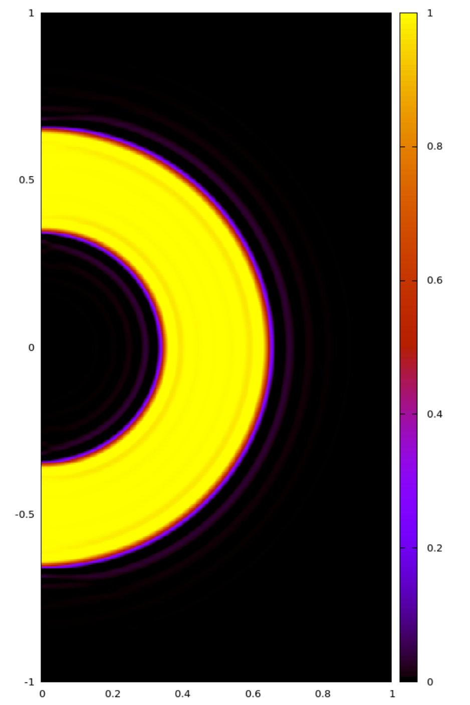 Figure 1
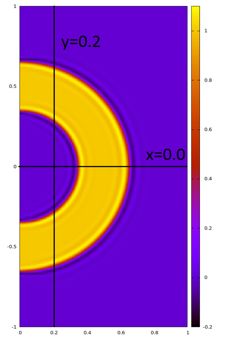 Figure 2
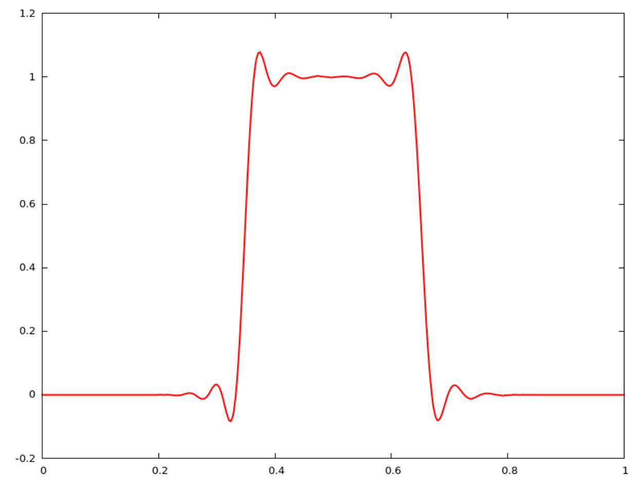 Figure 3
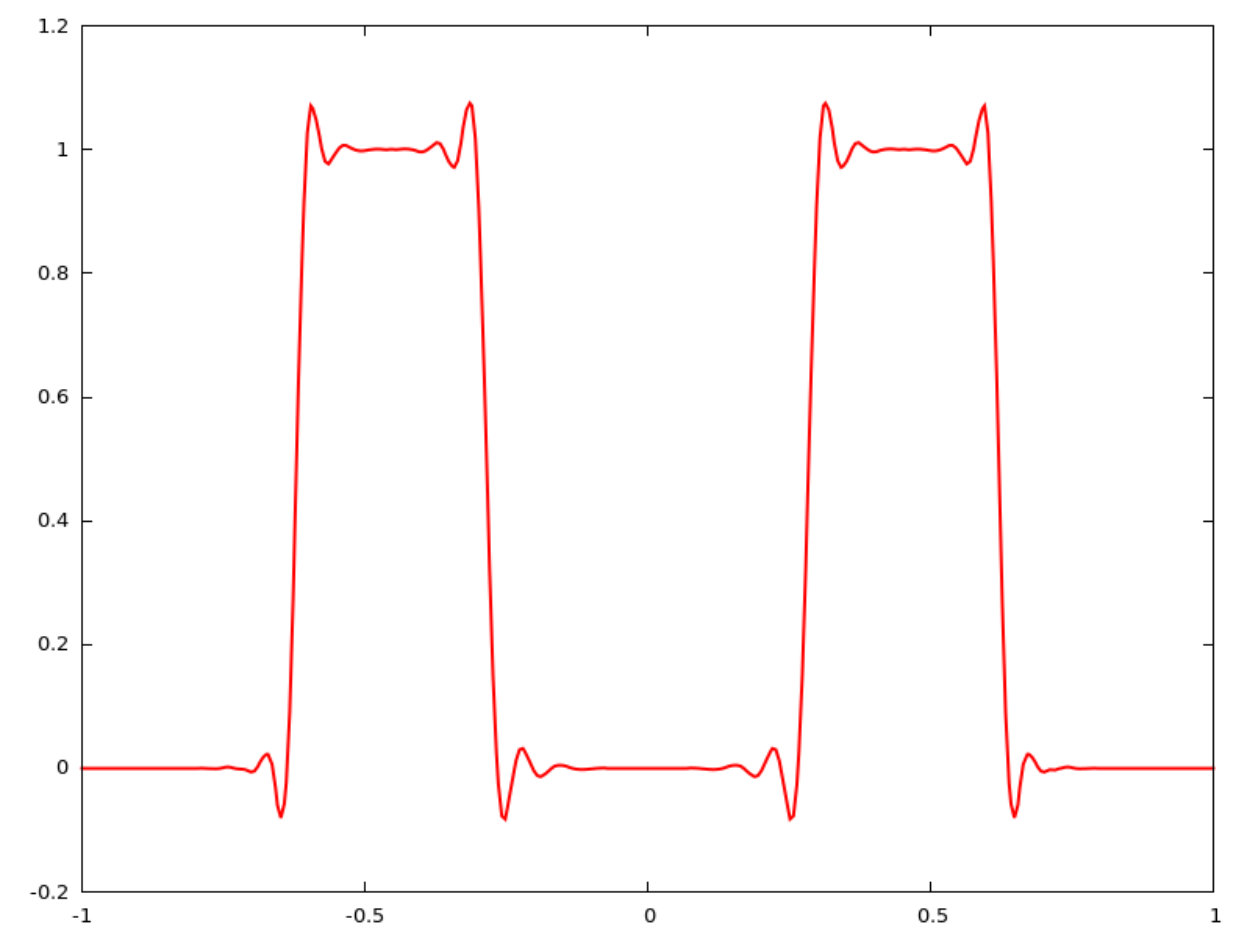 Figure 4
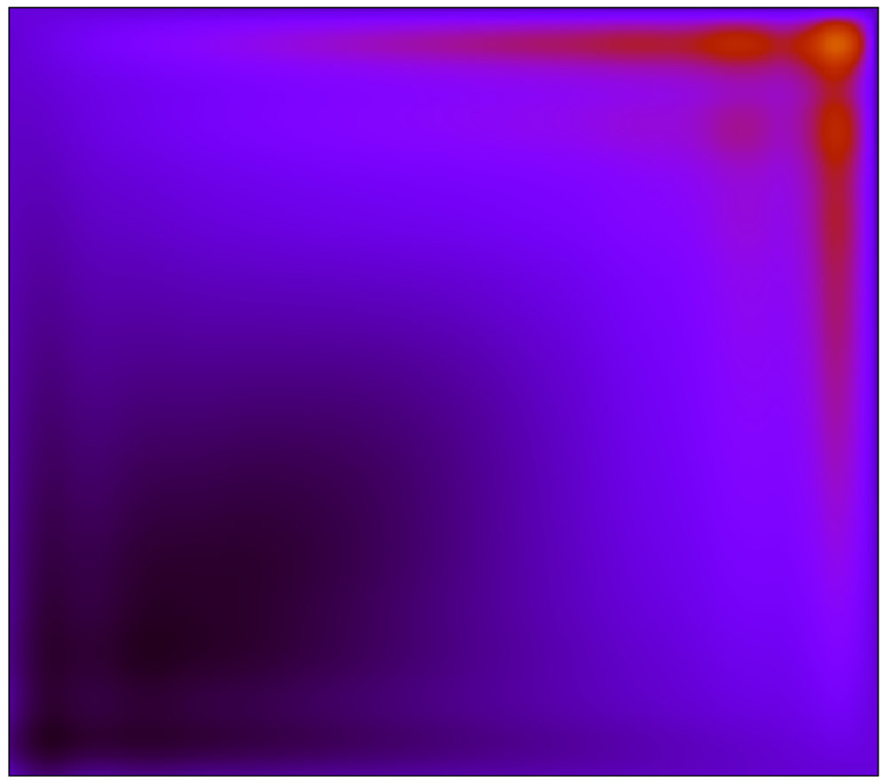 Figure 5
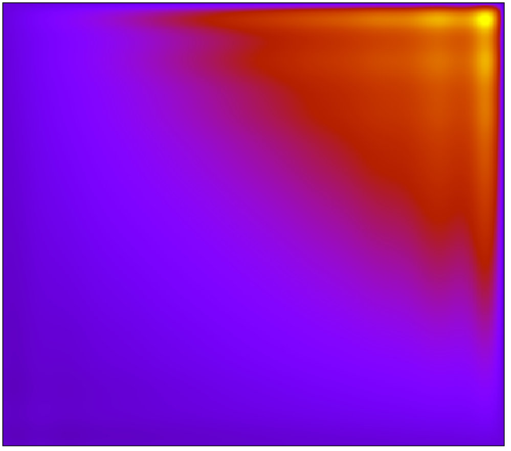 Figure 6
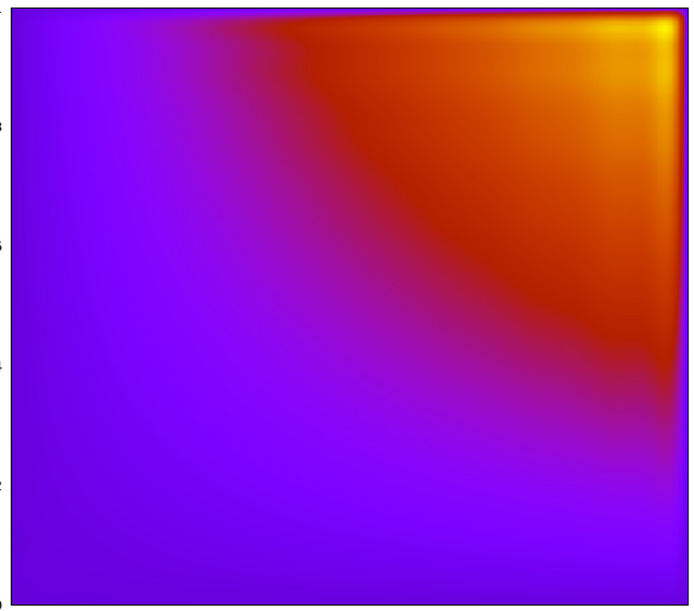 Figure 7
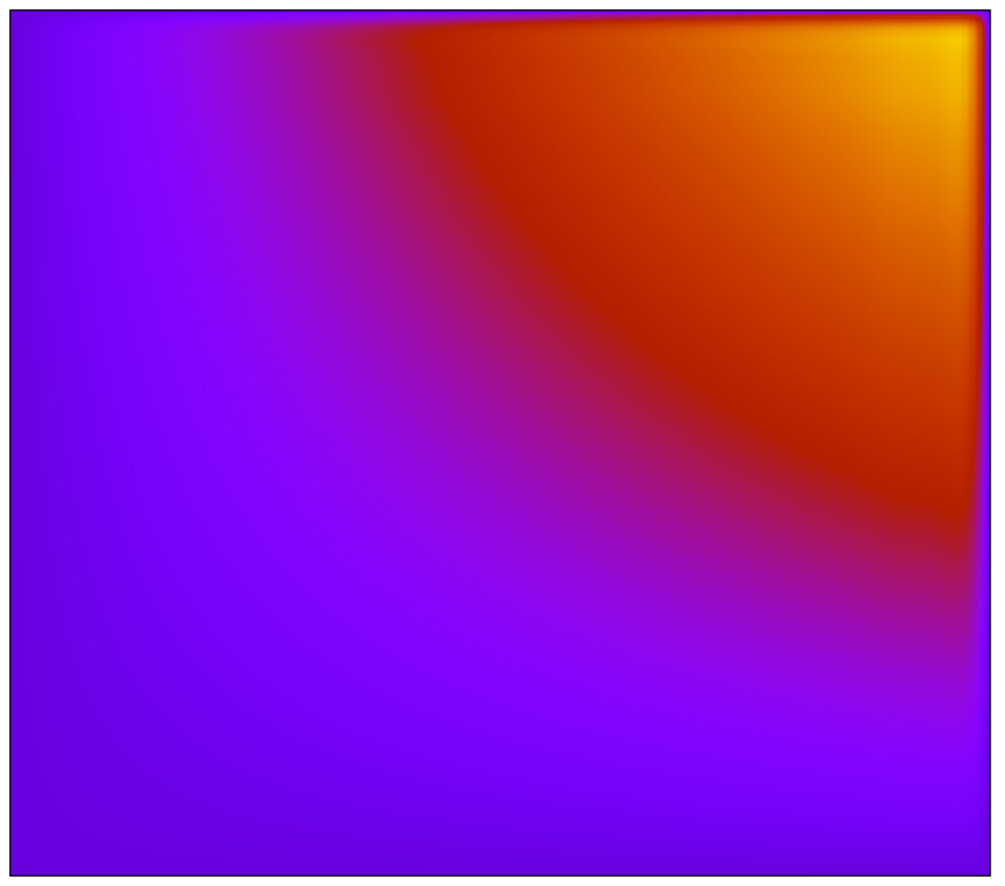 Figure 8
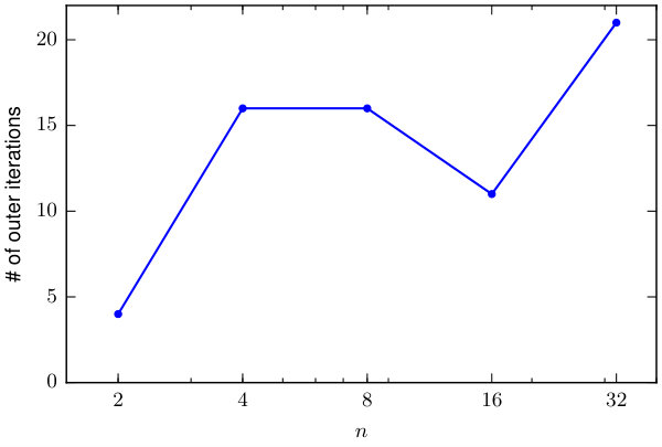 Figure 9
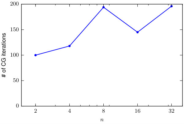 Figure 10
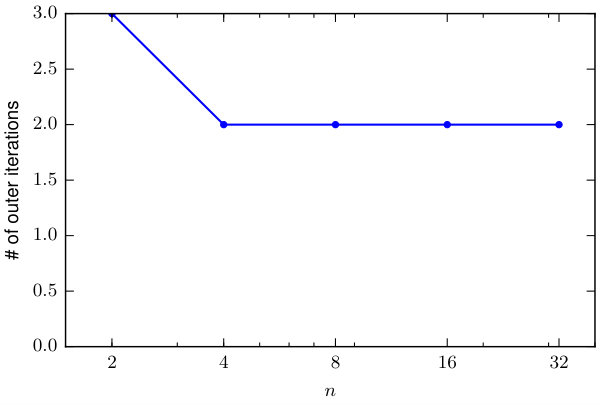 Figure 11
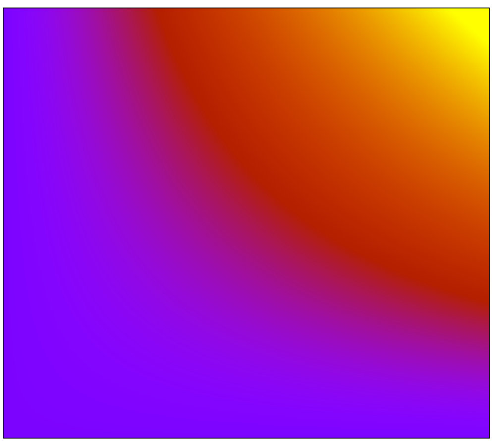 Figure 12
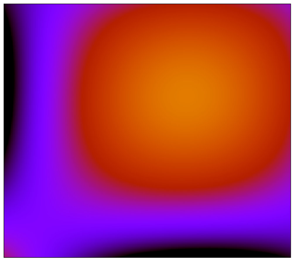 Figure 13
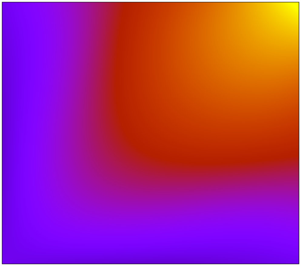 Figure 14
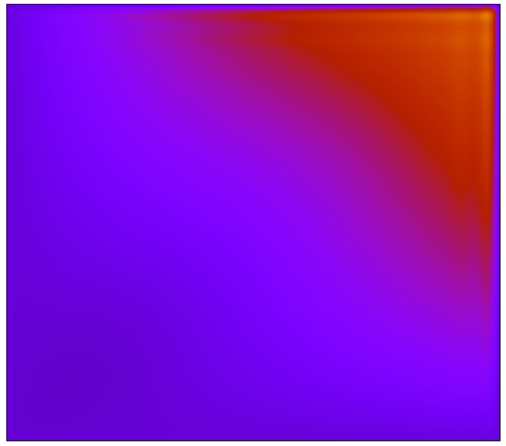 Figure 15
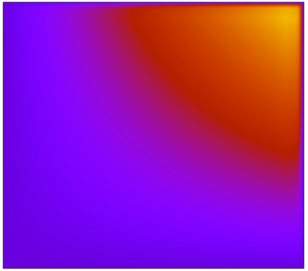 Figure 16
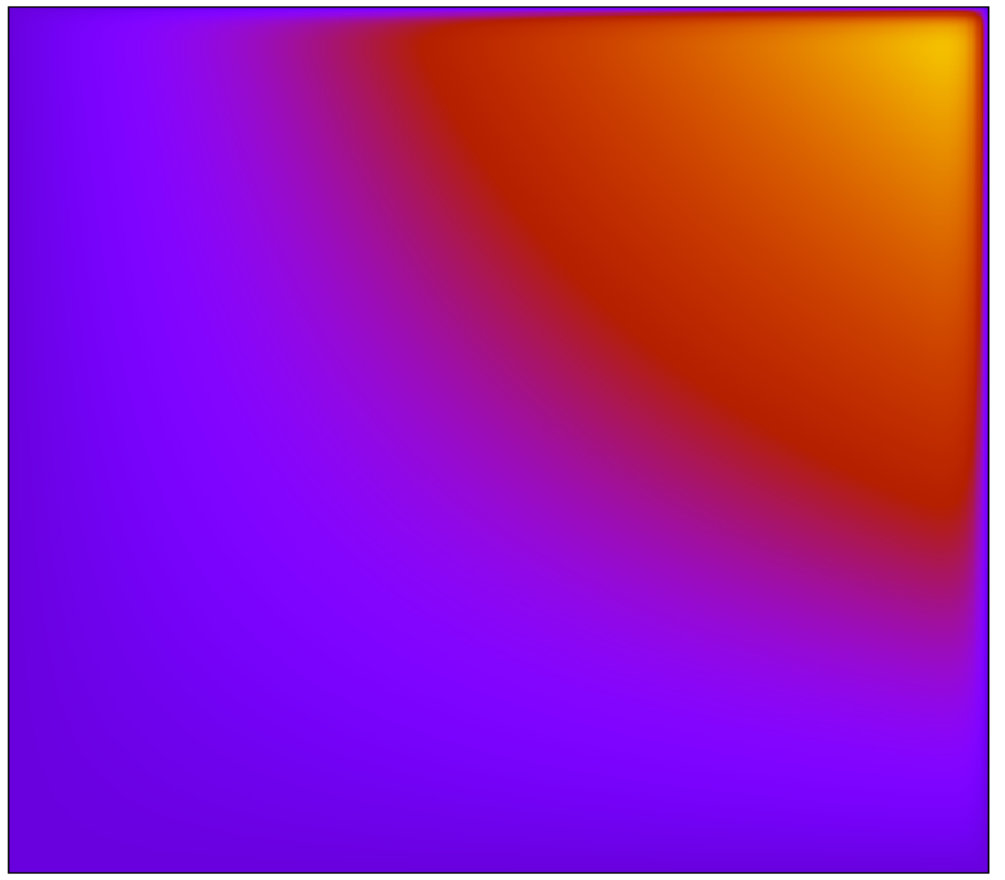 Figure 17
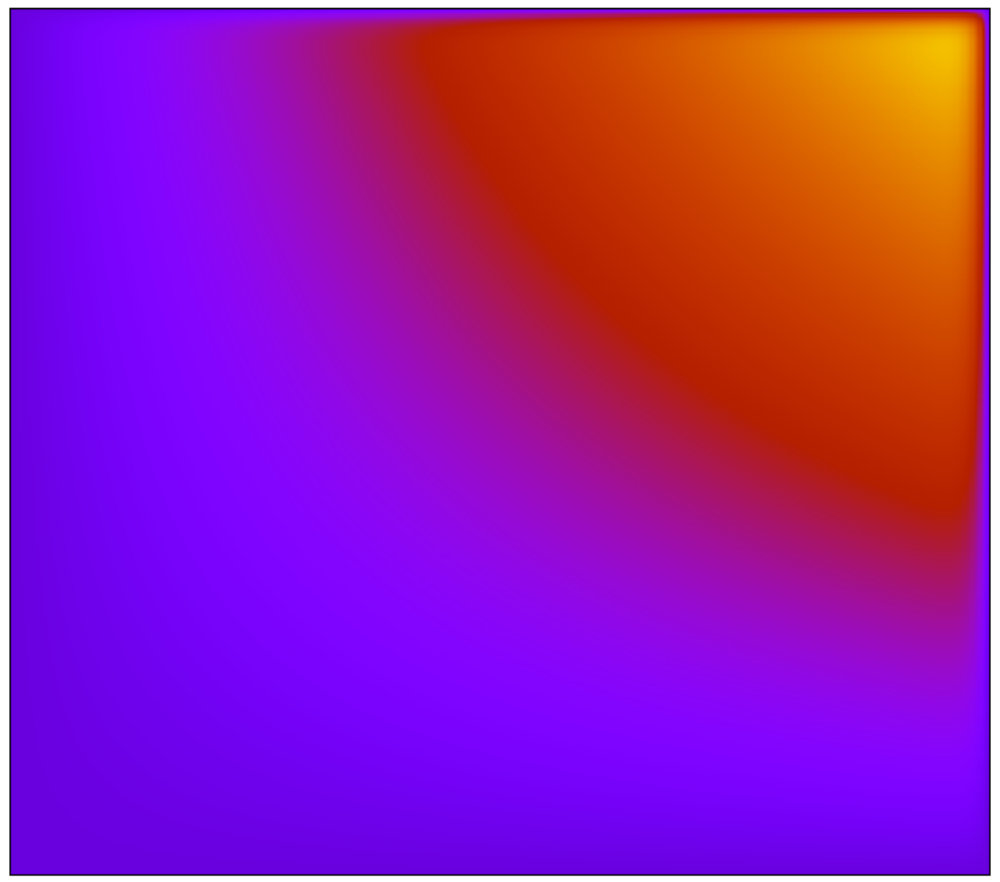 Figure 18
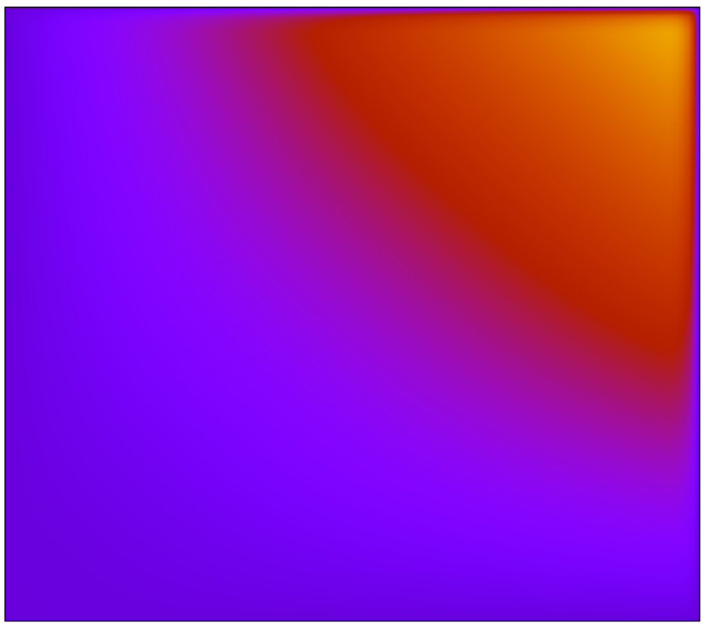 Figure 19
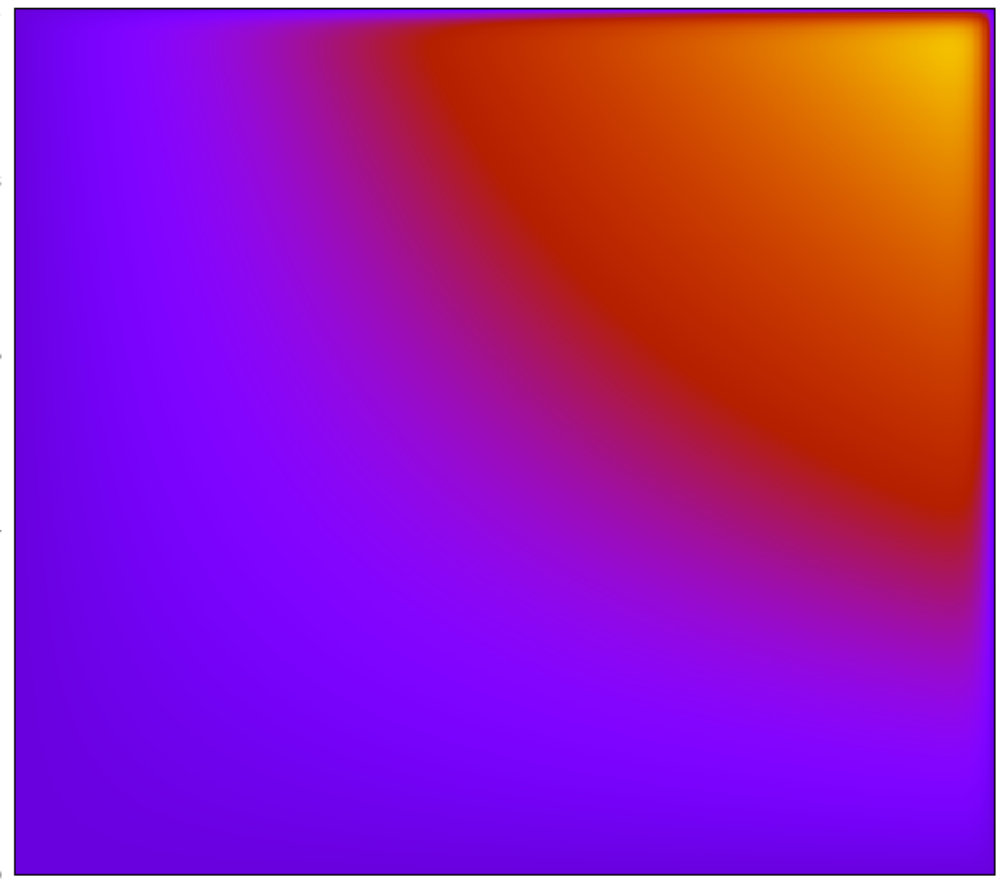 Figure 20
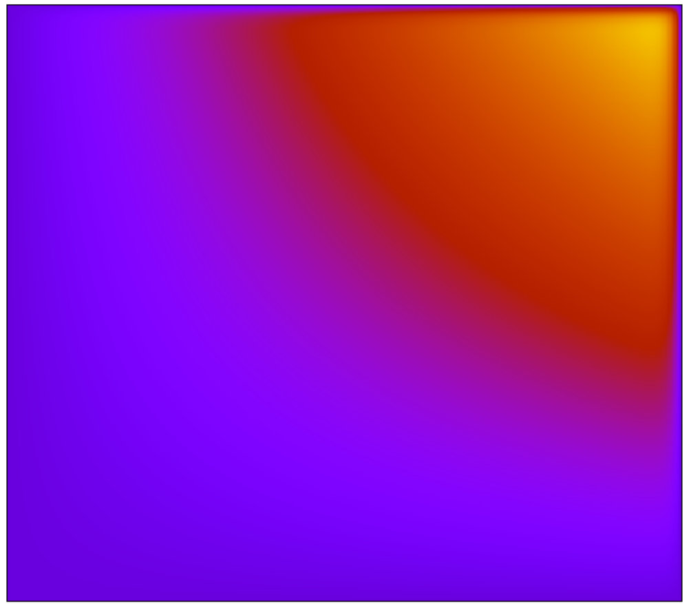 Figure 21
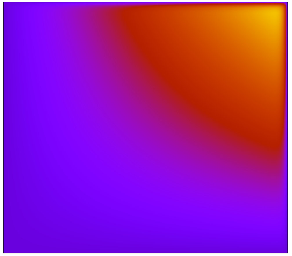 Figure 22
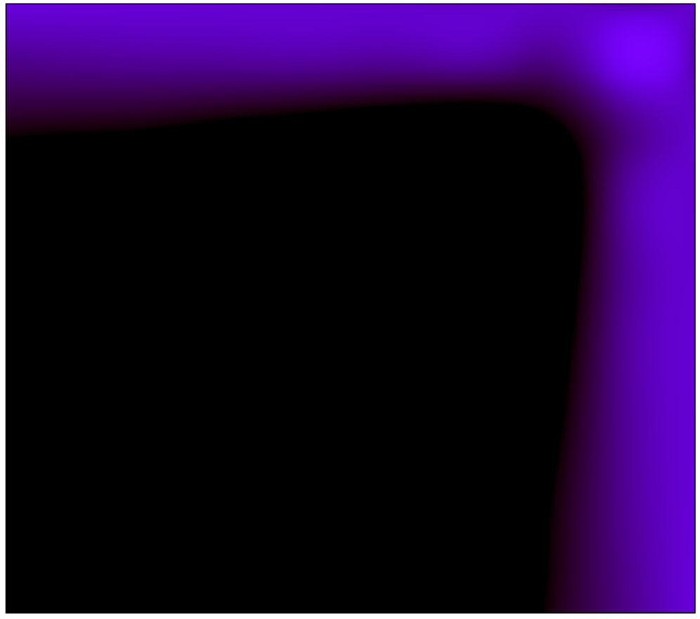 Figure 23
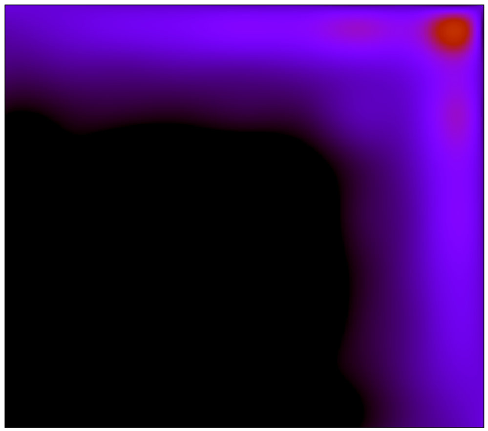 Figure 24
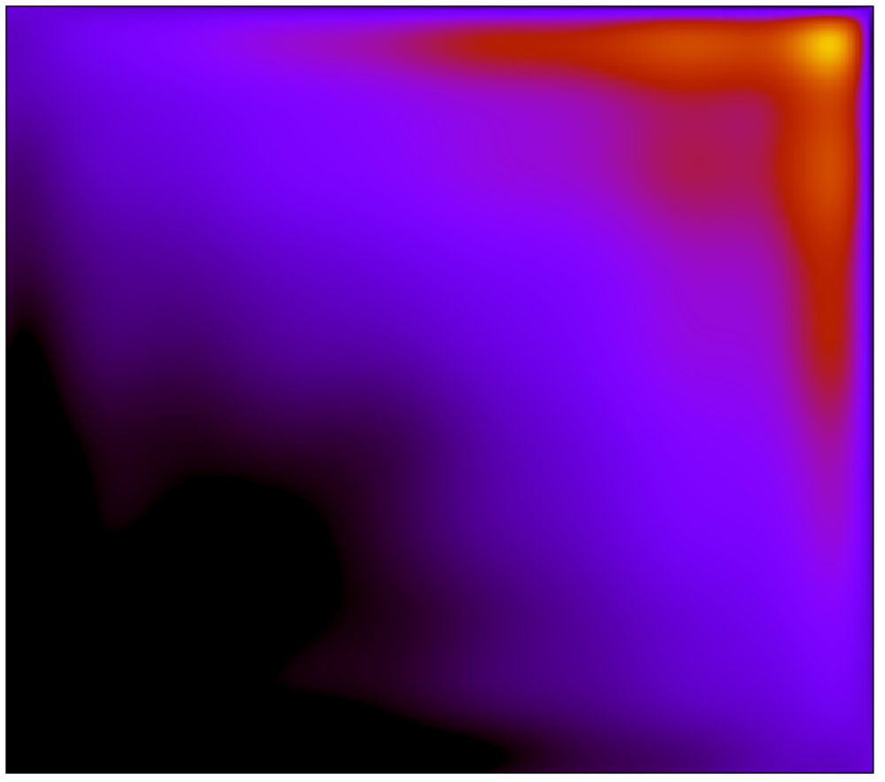 Figure 25
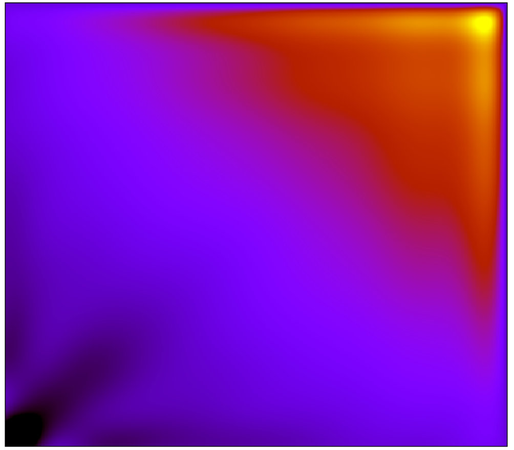 Figure 26
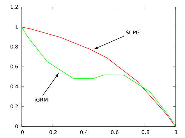 Figure 27
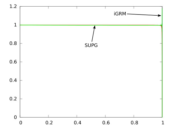 Figure 28
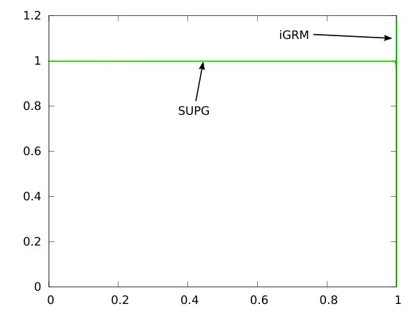 Figure 29
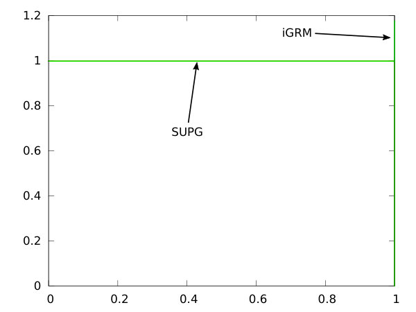 Figure 30
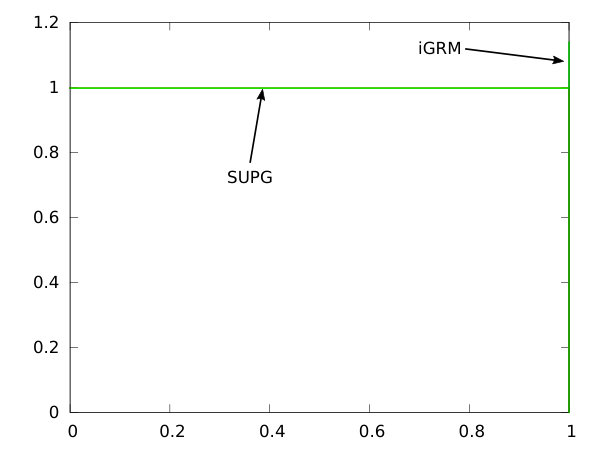 Figure 31
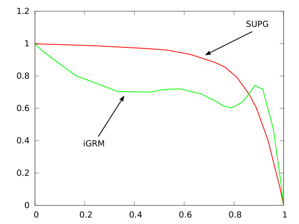 Figure 32
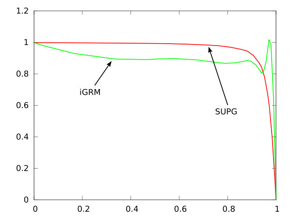 Figure 33
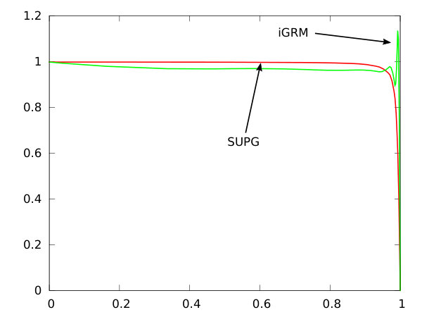 Figure 34
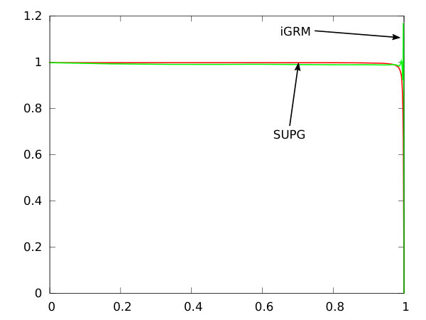 Figure 35
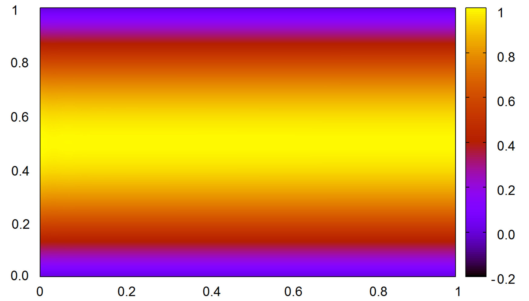 Figure 36
 Figure 37
 Figure 38
 Figure 39
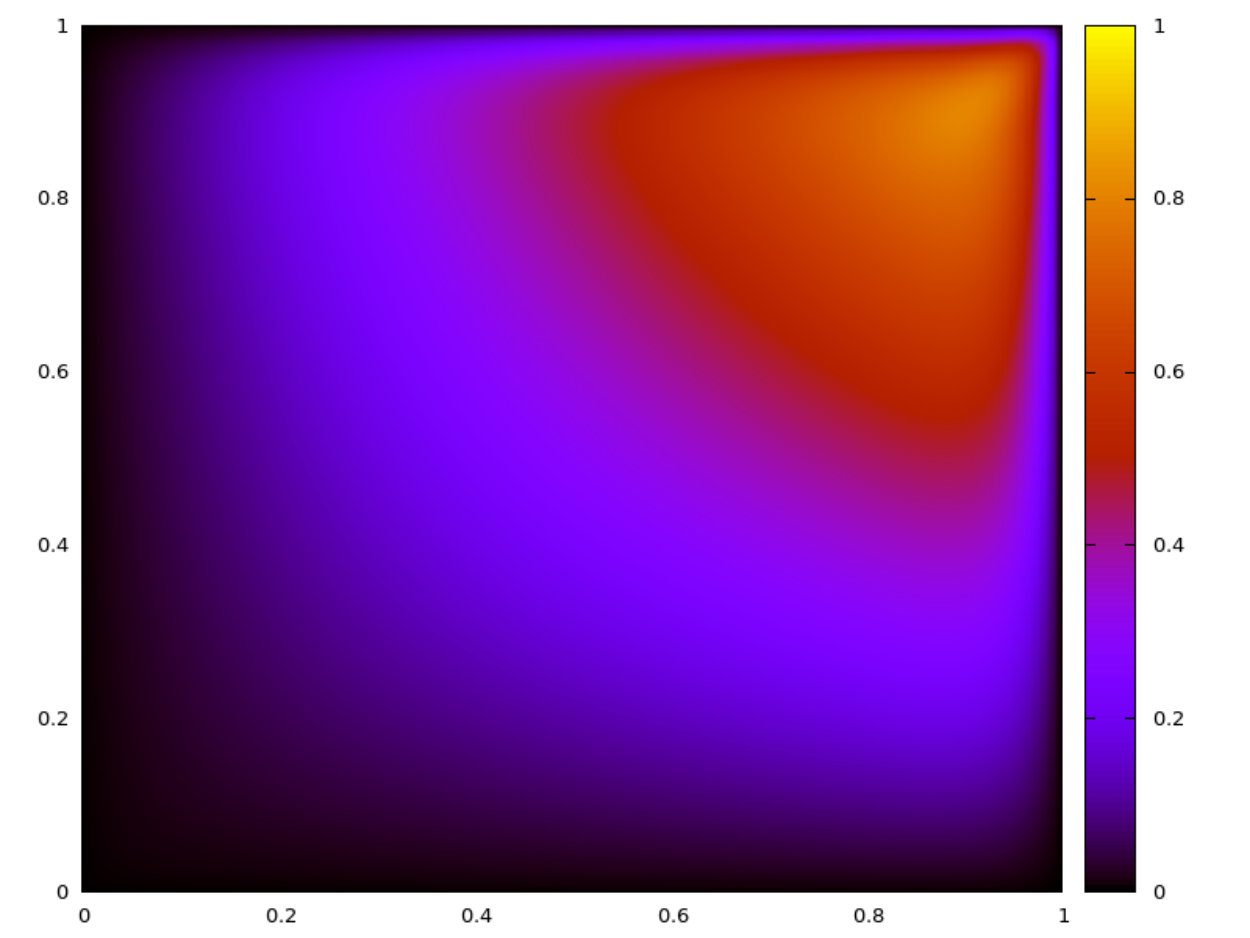 Figure 40
| n | trial (2,1) | trial (3,2) | trial (4,3) | trial (5,4) |
|---|---|---|---|---|
| test (2,0) | test (2,0) | test (2,0) | test (2,0) | |
| #DOF | 389 | 410 | 433 | 458 |
| L2 | 192.47 | 151.23 | 78.69 | 28.11 |
| H1 | 101.14 | 74.54 | 44.33 | 32.05 |
| #DOF | 1413 | 1450 | 1489 | 1530 |
| L2 | 80.01 | 16.64 | 3.29 | 1.48 |
| H1 | 59.56 | 29.83 | 18.04 | 10.40 |
| #DOF | 5381 | 5450 | 5521 | 5594 |
| L2 | 32.07 | 1.33 | 0.27 | 0.056 |
| H1 | 31.01 | 9.77 | 3.16 | 0.82 |
| #DOF | 20997 | 21130 | 21265 | 21402 |
| L2 | 7.66 | 0.07 | 0.01 | 0.003 |
| H1 | 9.86 | 1.67 | 0.26 | 0.068 |
| n | trial (2,1) | trial (3,2) | trial (4,3) | trial (5,4) |
|---|---|---|---|---|
| test (2,1) | test (3,2) | test (4,3) | test (5,4) | |
| #DOF | 100 | 121 | 144 | 169 |
| L2 | 40.36 | 38.74 | 38.72 | 38.82 |
| H1 | 73.30 | 80.16 | 82.86 | 83.72 |
| #DOF | 324 | 361 | 400 | 441 |
| L2 | 20.04 | 19.00 | 18.61 | 18.52 |
| H1 | 63.04 | 62.19 | 61.24 | 61.01 |
| #DOF | 1156 | 1225 | 1296 | 1369 |
| L2 | 6.51 | 5.07 | 4.20 | 3.66 |
| H1 | 36.57 | 26.88 | 21.16 | 17.35 |
| #DOF | 4356 | 4489 | 4624 | 4761 |
| L2 | 1.19 | 0.80 | 0.75 | 0.75 |
| H1 | 11.50 | 3.94 | 1.39 | 0.62 |
| iteration 1 [0 0.5 1] | iteration 3 [0 0.5 0.75 0.875 1] | iteration 5 [0 0.5 0.75 0.875 |
| 0.9375 0.96875 1] | ||
| iteration 7 [0 0.5 0.75 0.875 | iteration 9 [0 0.5 0.75 0.875 | iteration 11 [0 0.5 0.75 0.875 |
| 0.9375 0.96875 0.984375 1] | 0.9375 0.96875 … | 0.9375 0.96875 … |
| 0.998046875 1] | 0.998046875 0.9990234375 | |
| 0.9995117188 1] | ||
| iteration 13 [0 0.5 0.75 0.875 | iteration 15 [0 0.5 0.75 0.875 | iteration 17 [0 0.5 0.75 0.875 |
| 0.9375 0.96875 … | 0.9375 0.96875 … | 0.9375 0.96875 … |
| 0.9998779297 1] | 0.9998779297 0.9999389648 | 0.9998779297 0.9999389648 |
| 0.9999694824 1] | 0.9999694824 0.9999847412 | |
| 0.9999923706 1] |
| iteration 18 [0 0.5 0.75 | iteration 19 [0 0.5 0.75 | iteration 20 [0 0.5 0.75 |
| 0.875 0.9375 0.96875 … | 0.875 0.9375 0.96875 … | 0.875 0.9375 0.96875 … |
| 0.9999961853 1] | 0.9999980927 1] | 0.9999980927 0.9999990463 1] |
| iteration 21 [0 0.5 0.75 0.875 | iteration 22 [0 0.5 0.75 0.875 | iteration 23 [0 0.5 0.75 0.875 |
| 0.9375 0.96875 … | 0.9375 0.96875 … | 0.9375 0.96875 … |
| 0.9999990463 0.9999995232 1] | 0.9999990463 0.9999995232 | 0.9999990463 0.9999995232 |
| 0.9999997616 1] | 0.9999997616 0.9999998808 1] | |
| iteration 21 [0 0.5 0.75 0.875 | iteration 22 [0 0.5 0.75 0.875 | iteration 23 [0 0.5 0.75 0.875 |
| 0.9375 0.96875 … | 0.9375 0.96875 … | 0.9375 0.96875 … |
| 0.9999999404 1] | 0.9999999404 0.9999999702 1] | 0.9999999404 0.9999999702 |
| 0.9999999851 1] |
| SUPG (2,1) | iGRM (2,1) (3,1) | |||||
|---|---|---|---|---|---|---|
| iteration | #NRDOF | L2 | H1 | #NRDOF | L2 | H1 |
| 1 | 24 | 44.33 | 56.37 | 84 | 53.59 | 68.00 |
| 2 | 30 | 33.79 | 56.29 | 110 | 44.00 | 66.03 |
| 3 | 36 | 24.74 | 66.30 | 136 | 31.86 | 90.46 |
| 4 | 42 | 17.75 | 87.73 | 162 | 20.31 | 143.38 |
| 5 | 48 | 12.63 | 121.57 | 188 | 12.42 | 227.77 |
| 6 | 54 | 8.96 | 170.93 | 214 | 7.36 | 345.20 |
| 7 | 60 | 6.34 | 241.31 | 240 | 4.49 | 506.91 |
| 8 | 66 | 4.49 | 341.08 | 266 | 2.85 | 731.00 |
| 9 | 72 | 3.18 | 482.28 | 292 | 1.89 | 1044.11 |
| 10 | 78 | 2.26 | 681.99 | 318 | 1.31 | 1484.00 |
| 11 | 84 | 1.61 | 964.41 | 344 | 0.94 | 2103.96 |
| 12 | 90 | 0.70 | 1363.73 | 370 | 0.70 | 2979.06 |
| 13 | 96 | 0.84 | 1928.06 | 396 | 0.55 | 4026.87 |
| 14 | 102 | 0.63 | 1623.21 | 422 | 0.45 | 353.16 |
| 15 | 108 | 0.49 | 104.06 | 448 | 0.39 | 76.60 |
| 16 | 114 | 0.39 | 77.93 | 474 | 0.35 | 69.25 |
| 17 | 120 | 0.34 | 78.38 | 500 | 0.34 | 58.28 |
| 18 | 126 | 0.31 | 68.11 | 526 | 0.34 | 34.03 |
| 19 | 132 | 0.30 | 48.56 | 552 | 0.34 | 12.57 |
| 20 | 138 | 0.30 | 27.56 | 578 | 0.34 | 3.97 |
| 21 | 144 | 0.30 | 9.59 | 604 | 0.34 | 2.45 |
| 22 | 150 | 0.30 | 4.40 | 630 | 0.34 | 2.35 |
| 23 | 156 | 0.30 | 2.69 | 656 | 0.34 | 2.35 |
| 24 | 162 | 0.30 | 2.85 | 682 | 0.34 | 2.35 |
| 25 | 168 | 0.30 | 2.85 | 708 | 0.34 | 2.35 |
| iteration | # outer | # inner | L2 | H1 | time [ms] | |
|---|---|---|---|---|---|---|
| 1 | 0.1 | 12.76 | 225.88 | 37 | ||
| 1 | 0.01 | 10 | 32 | 24.95 | 166.275 | 12 |
| 1 | 0.001 | 4 | 18 | 49.86 | 73.11 | 6 |
| 1 | 0.0001 | 3 | 16 | 53.59 | 68.00 | 5 |
| 1 | 0.00001 | 2 | 12 | 58.90 | 66.36 | 4 |
| 1 | 0.000001 | 2 | 11 | 59.02 | 66.45 | 4 |
| 1 | 0.0000001 | 2 | 11 | 59.02 | 66.46 | 4 |
| 1 | 0.00000001 | 2 | 11 | 59.02 | 66.46 | 4 |
| 20 | 0.1 | 0.34 | 42.96 | 132 | ||
| 20 | 0.01 | 0.34 | 8.24 | 103 | ||
| 20 | 0.001 | 5 | 69 | 0.34 | 4.07 | 30 |
| 20 | 0.0001 | 2 | 51 | 0.34 | 3.97 | 21 |
| 20 | 0.00001 | 2 | 63 | 0.34 | 3.97 | 26 |
| 20 | 0.000001 | 2 | 65 | 0.34 | 3.97 | 23 |
| 20 | 0.0000001 | 2 | 81 | 0.59 | 4.05 | 31 |
| 20 | 0.00000001 | 2 | 85 | 4.73 | 8.91 | 34 |
Peer Reviews
No public reviews on file for this paper yet. If you reviewed it on a platform where reviews are public (OpenReview, ICLR, NeurIPS, ICML), you can paste yours below so the community can read it here.
Videos
No videos yet. Explain this paper in a talk, walkthrough, or lecture? Add one.
Isogeometric Residual Minimization Method (iGRM)
with Direction Splitting Preconditoner for Stationary Advection-Dominated Diffusion Problems
V.M.Calo, M. Łoś , Q.Deng, I. Muga, M. Paszyński
Department of Computer Science,
AGH University of Science and Technology, Krakow, Poland
e-mail: [email protected]
e-mail: [email protected]
Institute of Mathematics,
Pontifical Catholic Univeristy of Valparaíso, Chile
e-mail: [email protected]
Applied Geology, Faculty of Science and Engineering, Curtin University, Perth, WA, Australia,
e-mail: [email protected]
Mineral Resources, Commonwealth Scientific and Industrial Research Organisation (CSIRO),
Kensington, WA, Australia 6152
Abstract
In this paper, we introduce the isoGeometric Residual Minimization (iGRM) method. The method solves stationary advection-dominated diffusion problems. We stabilize the method via residual minimization. We discretize the problem using B-spline basis functions. We then seek to minimize the isogeometric residual over a spline space built on a tensor product mesh. We construct the solution over a smooth subspace of the residual. We can specify the solution subspace by reducing the polynomial order, by increasing the continuity, or by a combination of these. The Gramm matrix for the residual minimization method is approximated by a weighted norm, which we can express as Kronecker products, due to the tensor-product structure of the approximations. We use the Gramm matrix as a preconditional which can be applied in a computational cost proportional to the number of degrees of freedom in 2D and 3D. Building on these approximations, we construct an iterative algorithm. We test the residual minimization method on several numerical examples, and we compare it to the Discontinuous Petrov-Galerkin (DPG) and the Streamline Upwind Petrov-Galerkin (SUPG) stabilization methods. The iGRM method delivers similar quality solutions as the DPG method, it uses smaller grids, it does not require breaking of the spaces, but it is limited to tensor-product meshes. The computational cost of the iGRM is higher than for SUPG, but it does not require the determination of problem specific parameters.
keywords:
isogeometric analysis , residual minimization , iteration solvers , advection-diffusion simulations , linear computational cost , preconditioners
1 Introduction
We introduce the isoGeometric Residual Minimization (iGRM) method, which results in a stable discretization for advection-dominated diffusion problems. The method applies the residual minimization technique to stabilize the discrete solution. The minimum residual methods aim to find such that
[TABLE]
where and are Hilbert spaces, denotes the dual of , is a continuous bilinear (weak) form, is a discrete solution space, and is a given right-hand side. Several discretization techniques are particular incarnations of this wide-class of residual minimization methods. These include: the least-squares finite element method [19], the discontinuous Petrov-Galerkin method (DPG) with optimal test functions [20], the variational stabilization method [21], adaptive stabilized finite element method [39], or the automatic variationally stable finite element method [22]. This residual minimization technique exploits the tensor product structure of the discrete space to deliver Uzawa-like iteration schemes to solve the resulting global system. We approach the residual minimization as a saddle point (mixed) formulation, as described in [24].
The residual minimization method relies on the selection of the residual space and its inner product. In particular, we select a weighted norm as the inner product to obtain a Kronecker product structure of the Gramm matrix. This structure enables us to obtain a linear computational cost preconditioner for the Uzawa-like iterative solver. The resulting method converges well in the weighted norm.
For spatial discretization, we use IsoGeometric Analysis (IGA) [9]. IGA uses B-splines or NURBS [10] basis functions to construct a Galerkin finite element method (FEM). In particular, we use a tensor-product B-spline space to approximate the residual minimization method.
This structure enables for fast solution of the projection problem with isogeometric analysis [11, 12, 13]. A similar idea is applied to fast direction splitting solvers of explicit dynamics [14, 15, 16, 17, 18]. Splitting methods deliver fast factorizations as discussed, among many other sources, in [1, 2, 3, 4, 5, 6]. A modern version of this method solves different classes of problems [7, 8].
We exploit the Kronecker product structure of the approximated Gramm matrix to approximate the Schur complement, with iterative corrections in the outer loop. We approximate the inverse of the Schur complement system with a conjugate gradient solver (CG) [31] in the inner loop.
In this paper, we blend isogeometric analysis, residual minimization, and the alternating directions splitting solver. We solve the isogeometric Residual Minimization (iGRM) with a direction splitting preconditioner. We solve stationary advection-diffusion problems. We analyze four stationary computational problems, including a problem with the manufactured solution, the Eriksson-Johnson model problem, and a vortical wind problem. We use the Streamline Upwind Petrov-Galerkin (SUPG) and Discontinuous Petrov-Galerkin methods as references to compare the performance of our method.
The structure of the paper is the following. We start from the introduction of the iGRM method in Section 2. Next, in Section 3, we describe the general idea and the details of the iterative solver. In Section 4, we present the numerical results for the manufactured solution problem, Erikkson-Johnson model problem, and the vortical wind problem. We conclude with Section 5.
2 The Isogeometric Residual Minimization Method (iGRM)
To simplify the discussion, we focus on a two-dimensional model problem in space. Nevertheless, the extension of the formulation to three-dimensions is straightforward. We introduce a continuous bilinear (weak) form defined over solution and residual Hilbert spaces, and a given right-hand side, where denotes the dual of .
2.1 Residual minimization method for the global problem
For a general weak problem: Find such as
[TABLE]
we define the operator
[TABLE]
such that
[TABLE]
to reformulate the problem as
[TABLE]
We minimize the residual
[TABLE]
We define the Riesz representer as
[TABLE]
We then project the problem back to
[TABLE]
We use here the definition of the dual norm
[TABLE]
The definition of the dual norm implicitly depends on the norm. Thus, a vital ingredient of a residual minimization method is the selection of a norm on . The quality of the results strongly depends on the choice for the norm on . The minimum is attained at when the Gâteaux derivative is equal to [math] in all directions: we define the operator
[TABLE]
We define the Riesz representation of the residual . Thus, our problem reduces to
[TABLE]
The action of the inverse of the Riesz operator on the functional is equal to that element itself in . Therefore, we get
[TABLE]
From the definition of the error representation in terms of the residual, we have
[TABLE]
Thus, our problem reduces to the following semi-infinite problem: Find such that
[TABLE]
We discretize the residual space as to obtain the discrete problem: Find such as
[TABLE]
where is the inner product in inherited from , , .
Remark 1**.**
We define the discrete residual space to be sufficiently close to the continuous space to ensure stability. Indeed, we gain stability by enriching the residual space (while fixing the solution space ) until we reach the discrete inf-sup stability.
2.2 Minimal residual discretization for the global problem with
B-splines
We approximate the solution with a tensor product of one-dimensional B-splines. We choose a uniform order in all directions to simplify the discussion.
We denote the basis functions in the -direction for the discrete solution and residual spaces as and , respectively. Similarly, we denote the basis functions in the -direction for the discrete solution and residual spaces as and , respectively.
We approximate the residual space with a sufficiently larger discrete space than the solution space to guarantee discrete stability (cf. [39]). We achieve this by either increasing the polynomial order or decreasing the continuity of the residual space to define the solution space. As a result, we now can define the discrete solution and residual functions as:
[TABLE]
and the discrete solution and residual functions as
[TABLE]
3 Conjugate Gradients method for Schur complement
In this section, we derive an iterative solution algorithm for the residual minimization problem. We denote by a bounded open set of with Lipschitz continuous boundary , where . We assume that the domain has a tensor product structure. This structure allows us to approximate the Gramm matrix as a Kronecker product of one-dimensional matrices.
The resulting matrix system for the residual minimization method is
[TABLE]
where we minimize the isogeometric discretization residual of (14) in the energy norm (a weighted norm), where is defined as
[TABLE]
where we keep the weight as a solver parameter, and
[TABLE]
where , and denote 1D mass matrices and stiffness matrices, respectively, defined as
[TABLE]
We approximate the Gramm matrix in the residual minimization as a Kronecker product matrix , that is inexpensive to solve (it requires solutions of two one-dimensional problems with multiple right-hand sides, where the sizes of the problems and the number of right-hand-sides corresponds to the mesh dimensions in both directions) and only introduces an error of order {\color[rgb]{0,0,0}\definecolor[named]{pgfstrokecolor}{rgb}{0,0,0}\pgfsys@color@gray@stroke{0}\pgfsys@color@gray@fill{0}\eta^{2}}. From (18), we have
[TABLE]
where .
The definition of the matrix in (17) corresponds to applying an appropriate isogeometric weak form of the scalar field PDE.
3.1 Overview of the iterative algoritm
In this section, we describe the iterative algorithm. Given an initial guess , we compute the update as
[TABLE]
Thus
[TABLE]
This system of linear equations is expensive to factorize, so we use the approximate
[TABLE]
We propose the following iterative algorithm
3.2 Convergence of the iterative algorithm
Since the Algorithm 1 uses a preconditioned CG and both the CG and preconditioned CG are convergent (see, for example, [31]), we focus on the spectral analysis of (21) in Algorithm 1.
Applying the initialization , we obtain
[TABLE]
where is the update of .
We now have
[TABLE]
To simplify the spectral analysis and without loss of generality, we set . Thus, combining (22) and (23) gives
[TABLE]
Now, we analyze the spectrum of
[TABLE]
We apply a spectral decomposition [32] to the matrix with respect to and arrive at
[TABLE]
where is a diagonal matrix with entries to be the eigenvalues of the generalized eigenvalue problem
[TABLE]
and the columns of are the eigenvectors. We assume that all the eigenvalues are sorted in ascending order and are listed in and the -th column of is associated with the eigenvalue .
Using (26) and (25), we now calculate
[TABLE]
where
[TABLE]
We assume here that the mesh is uniform in both directions.
Thus, similarly, we have
[TABLE]
The middle term is a diagonal matrix. Thus, a typical eigenvalue of is
[TABLE]
where are indices of eigenvalues in each dimension. The spectral radius of is then
[TABLE]
where are the maximum eigenvalues in each dimension. Immediately, we have
[TABLE]
Thus, the eigenvalues of the amplifying block-matrix (the vector in terms of is from inner CG) in (24) are 1 and . Thus, they are bounded by 1, which implies that the eigenvalues of their powers are also bounded by 1. Hence, the iterative Algorithm 1 is convergent.
4 Numerical results for stationary problems
In this section, we focus on a model advection-diffusion problem defined as follows. For a unitary square domain , the advection vector and the diffusion coefficient , we seek the solution of the advection-diffusion equation
[TABLE]
with Dirichlet boundary conditions on the whole boundary of . We partition the boundary into the inflow and the outflow .
We introduce the discrete weak formulation
[TABLE]
[TABLE]
where is the vector normal to , and is the “normal” elemental distance (i.e., mesh size in the direction of the normal) (possibly changing with elements of the mesh),
[TABLE]
where the gray and red represent the penalty terms, and corresponds to the forcing term, while the brown terms result from the integration by parts [36].
In our model problem, we seek the solution in space . The inner product in is defined as weighted norm (18).
A popular stabilization technique is the Streamline-upwind Petrov-Galerkin (SUPG) method [26, 25]. This method modifies the weak form as follows
[TABLE]
where , and , where stands for the diffusion term, and for the convection term, and and are horizontal and vertical dimensions of an element . Thus, we have
[TABLE]
[TABLE]
[TABLE]
4.1 A manufactured solution problem
First, we select the advection vector , and and solve the advection-diffusion equation (34) with homogeneous Dirichlet boundary conditions. We utilize a manufactured solution enforced by the forcing term . This analytic expression of the solution limits the Péclet number to due to machine precision.
We use the weak form (35) and the inner product (18) into the iGRM setup (14) and use the preconditioned CG solver described in Section 3. In the weighted norm we introduce , where is the diameter of the element.
In the following problem, we study the - and -convergence of the iGRM method on uniform grids using different combinations of solution and residual spaces. We do not employ adaptive Shishkin grids here [23]. We increase the accuracy by increasing the order and continuity of solution spaces (-increase [9, 38]) simultaneously. Increasing solution space order and continuity improves the accuracy of the solution for this smooth problem. Similarly, refining the mesh also improves the accuracy of the solution.
Table 1 illustrates the and -convergence of the method. The rows represent -refinement of the solution test, from (order , continuity ) to (order , continuity p), and the columns represent -refinement, from mesh to mesh. We report the numbers of degrees of freedom and the error in and norms.
The black colors on the numerical results represent unwanted negative values of the solution. We can read from Table 1 that -refinement (increasing polynomial order of the solution with maximum continuity) is more attractive than -refinement since the solution improves using fewer degrees of freedom.
We also present in Table 2 the results for SUPG method for the corresponding meshes and approximation spaces. We conclude that we can achieve less than 1 percent error, as measured in and norms, for iGRM method for for trial (5,4) test (2,0) over mesh, and for SUPG method for for trial=test=(5,4) over mesh.
4.2 Erikkson-Johnson model problem
We focus now on the model Eriksson-Johnson problem with the modifications proposed by [24]. For the square domain and the advection vector , we seek the solution of the advection-diffusion equation (34). We introduce the Dirichlet boundary conditions
[TABLE]
[TABLE]
weakly on the boundary . The inflow Dirichlet boundary condition drives the problem and it develops a boundary layer of width at the outflow .
In the manufactured solution problem, we compare the SUPG and iGRM methods on a sequence of uniform grids. Later, we compare iGRM and SUPG methods on a sequence of adapted grids. We simulate the Erikkson-Johnson problem with the iGRM and SUPG methods with on a sequence of grids refined towards the boundary layer. We start from the uniform grid of elements, and we add the knot points to the last interval on the right in the direction. We refine the knot vector in the direction by breaking in half the rightmost element. We continue to refine in the perpendicular direction after we capture the boundary layer when the element size in one direction is below .
We illustrate the solutions obtained from the iGRM and SUPG methods in Figures 3-1. We report the convergence in and norms in Table 5.
We now compare iGRM vs the DPG method [24] using Lagrange (2,0) polynomials for solution and (3,0) polynomials for the residual. In our method, we use a (2,1) space for the solution with either a (3,1) or (3,2) space for the residual. Thus, our solution spaces have identical order and higher continuity, so they are smaller than those used in [24].
We compare the iGRM computations with the DPG results from Figure 5.3 in [24], which shows the errors. Both iGRM and DPG meshes are adapted. The DPG method [24] for delivers an norm error of order 0.02 for mesh size of the order 2000. The iGRM method for mesh dimension delivers norm error 0.02 on mesh size 1312 with a residual space of (3,1). Summing up, for , iGRM delivers similar quality solutions on smaller grids. We achieve this by using smooth functions with higher continuity approximations. Additionally, the iGRM implementation is simpler since it does not require breaking the spaces. Nevertheless, the present solution strategy for iGRM is limited to tensor-product meshes.
Comparing the iGRM with SUPG, we conclude that iGRM converges to similar quality solutions than the SUPG method. The computational cost is higher for iGRM, but the iGRM method does not require the determination of problem-specific parameters.
We also investigate the convergence and the execution times of the iterative solver. We show in Table 6 the dependence of the number of iterations of the inner and outer loops on the parameter from the definition of the inner product. We use the Erikkson-Johnson problem as a reference. We implement the iGRM code in the IGA-ADS software [17], which automatically uses all cores of the machine. We run the experiments on Intel i7 processor with 2.7GHz with 8 cores and 16 GB of RAM.
4.3 Vortical wind problem
We now solve a vortical flow with the advection-dominated diffusion equations over the rectangular domain , with zero right-hand side , the advection vector . This velocity field is modeling a rotating flow. We introduce , . The Dirichlet boundary conditions are
[TABLE]
We use the iGRM setup (14) with the preconditioned CG solver described in Section 4. We use mesh with solution (2,1) residual (2,0). We use a Péclet number . The numerical results are summarized in Figures 2-4.
There are some overshoots and undershoots in the cross-sections of the mesh. They can be removed by performing mesh refinements. They can be also removed by using penalty methods [42, 43].
Remark 2**.**
The number of iterations of the conjugate gradient solver grows with the problem size, as presented in Table 6. We will explore possible solutions to this issue in future work. The computational cost of the solver grows like where is the number of degrees of freedom, and is the number of iterations.
5 Conclusions
We introduce a stabilized isogeometric method that uses residual minimization in a dual norm. We design the method to achieve good solution properties. The method exploits the Kronecker product structure of the computational problem to deliver fast solutions. The solution space in our scheme uses maximum continuity B-splines. To accelerate the solution of the algebraic scheme, we introduce a fast solver for the Gramm matrix, but without a Schur complement preconditioner. We call our method isogeometric residual minimization (iGRM) with direction splitting preconditioner. We verify the accuracy of the solution on four stationary problems. In this method, the diffusion and advection coefficient functions can be arbitrary. Our future work will extend this method to other problems, such as the Stokes [27] and Maxwell problems [28, 29, 30], the development of the method for time-dependent problems [37], as well as the development of the parallel software dedicated to the simulations of different non-stationary problems with the iGRM method. We will seek to find a proper preconditioner for the CG problem as well as an alternative method to speed up the solution of the saddle-point problem that the residual minimization delivers, e.g., based on [40, 41].
Acknowledgments
The National Science Centre, Poland, partially supported this work, grant no. 2017/26/M/ ST1/ 00281. This publication was also made possible in part by the CSIRO Professorial Chair in Computational Geoscience at Curtin University and the Deep Earth Imaging Enterprise Future Science Platforms of the Commonwealth Scientific Industrial Research Organisation, CSIRO, of Australia. Additional support was provided by the European Union’s Horizon 2020 Research and Innovation Program of the Marie Skłodowska-Curie grant agreement No. 777778. At Curtin University, support was provided by The Institute for Geoscience Research (TIGeR) and by the Curtin Institute for Computation.
The reference list from the paper itself. Each links out to its DOI / PubMed record.
- 1[1] A. A. Samarskij, E. S. Nikolaev, Numerical Methods for Grid Equations: Volume II Iterative Methods, Birkhäuser, Basel, Boston, Berlin (2012)
- 2[2] A. Quarteroni, R. Sacco, F. Saleri, Numerical Mathematics (Texts in Applied Mathematics) 2nd Edition, Springer, Berling, Heidelberg, New, York (2006)
- 3[3] D.W. Peaceman, H.H. Rachford Jr., The numerical solution of parabolic and elliptic differential equations, Journal of Society of Industrial and Applied Mathematics 3 (1955) 28–41.
- 4[4] J. Douglas, H. Rachford, On the numerical solution of heat conduction problems in two and three space variables, Transactions of American Mathematical Society 82 (1956) 421–439.
- 5[5] E.L. Wachspress, G. Habetler, An alternating-direction-implicit iteration technique, Journal of Society of Industrial and Applied Mathematics 8 (1960) 403–423.
- 6[6] G. Birkhoff, R.S. Varga, D. Young, Alternating direction implicit methods, Advanced Computing 3 (1962) 189–273.
- 7[7] J. L. Guermond, P. Minev, A new class of fractional step techniques for the incompressible Navier-Stokes equations using direction splitting, Comptes Rendus Mathematique 348(9-10) (2010) 581–585.
- 8[8] J. L. Guermond, P. Minev, J. Shen, An overview of projection methods for incompressible flows, Computer Methods in Applied Mechanics and Engineering, 195 (2006) 6011–6054.