TL;DR
This paper introduces Deep Progressive Quantization (DPQ), a novel neural network-based approach for image retrieval that learns quantization codes sequentially, enabling efficient training for multiple code lengths and outperforming existing methods.
Contribution
The paper proposes a deep progressive quantization model that learns quantization codes sequentially, allowing simultaneous training for various code lengths and improving retrieval performance.
Findings
DPQ outperforms state-of-the-art image retrieval methods.
DPQ requires less computation time due to single training for multiple code lengths.
Ablation studies confirm the effectiveness of each component.
Abstract
Product Quantization (PQ) has long been a mainstream for generating an exponentially large codebook at very low memory/time cost. Despite its success, PQ is still tricky for the decomposition of high-dimensional vector space, and the retraining of model is usually unavoidable when the code length changes. In this work, we propose a deep progressive quantization (DPQ) model, as an alternative to PQ, for large scale image retrieval. DPQ learns the quantization codes sequentially and approximates the original feature space progressively. Therefore, we can train the quantization codes with different code lengths simultaneously. Specifically, we first utilize the label information for guiding the learning of visual features, and then apply several quantization blocks to progressively approach the visual features. Each quantization block is designed to be a layer of a convolutional neural…
Click any figure to enlarge with its caption.
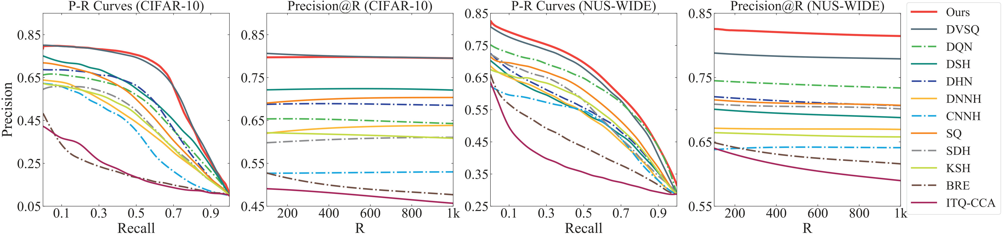 Figure 1
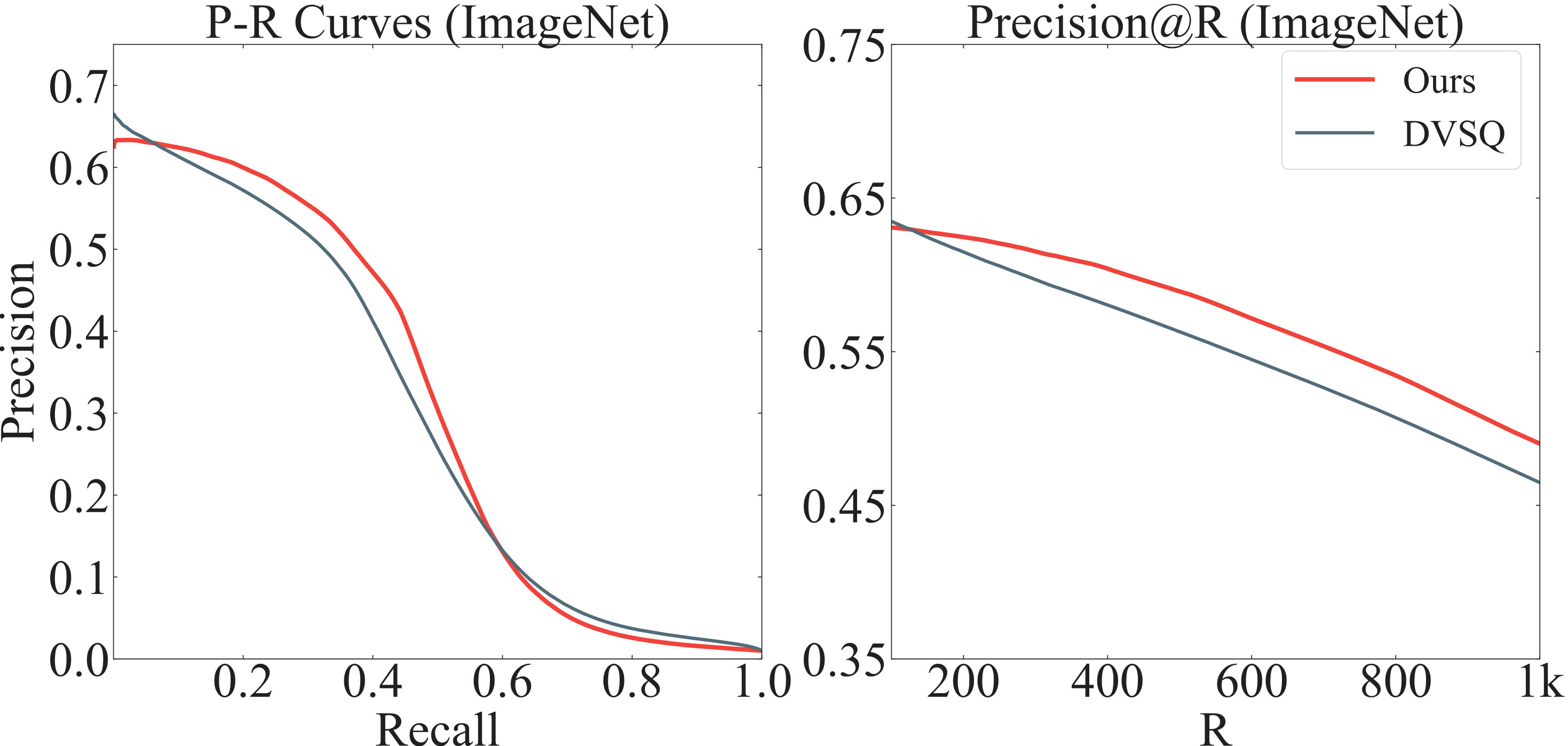 Figure 2
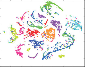 Figure 3
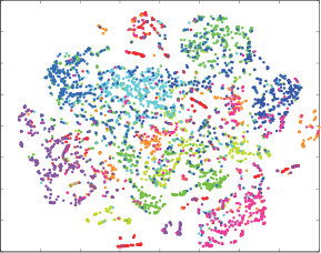 Figure 4
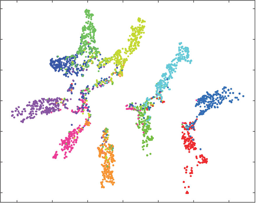 Figure 5
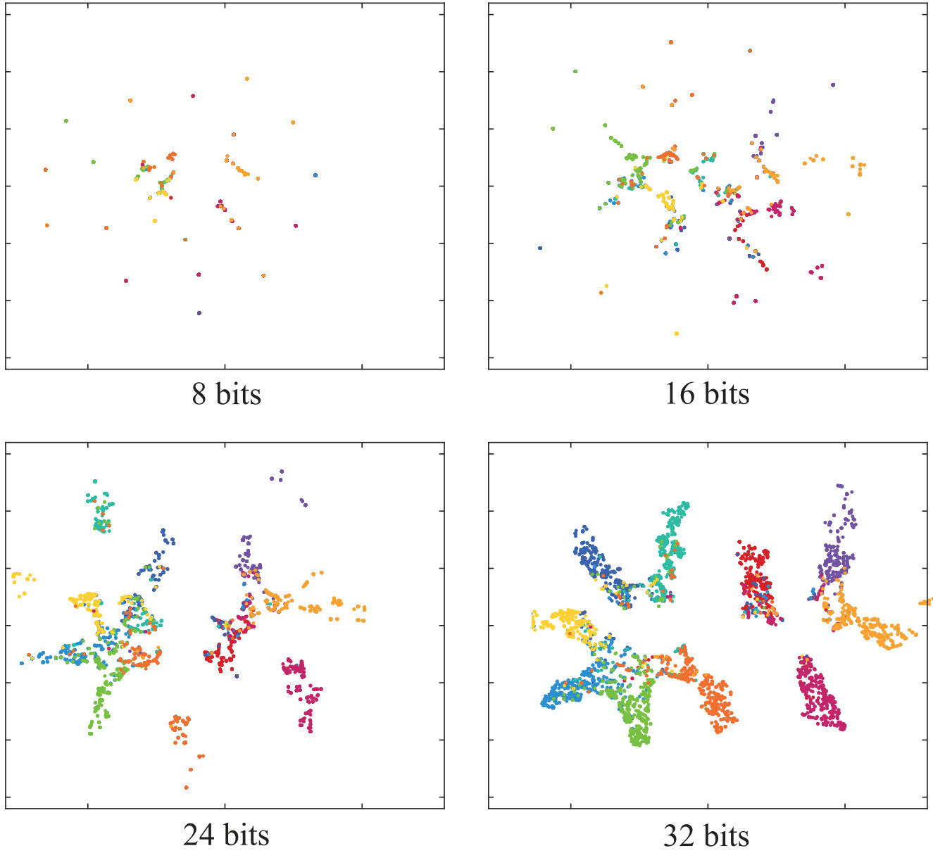 Figure 6
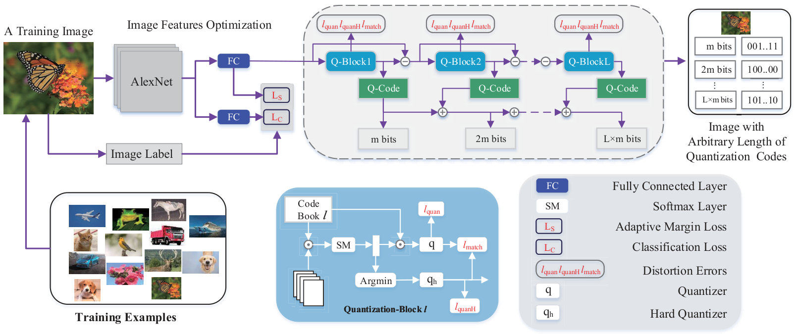 Figure 7
| Method | CIFAR-10 | NUS-WIDE | ImageNet | |||||||||
|---|---|---|---|---|---|---|---|---|---|---|---|---|
| 8 bits | 16 bits | 24 bits | 32 bits | 8 bits | 16 bits | 24 bits | 32 bits | 8 bits | 16 bits | 24 bits | 32 bits | |
| ITQ-CCA Gong et al. (2013) | 0.315 | 0.354 | 0.371 | 0.414 | 0.526 | 0.575 | 0.572 | 0.594 | 0.189 | 0.270 | 0.339 | 0.436 |
| BRE Kulis and Darrell (2009) | 0.306 | 0.370 | 0.428 | 0.438 | 0.550 | 0.607 | 0.605 | 0.608 | 0.251 | 0.363 | 0.404 | 0.453 |
| KSH Liu et al. (2012) | 0.489 | 0.524 | 0.534 | 0.558 | 0.618 | 0.651 | 0.672 | 0.682 | 0.228 | 0.398 | 0.499 | 0.547 |
| SDH Shen et al. (2015) | 0.356 | 0.461 | 0.496 | 0.520 | 0.645 | 0.688 | 0.704 | 0.711 | 0.385 | 0.516 | 0.570 | 0.605 |
| SQ Martinez et al. (2014) | 0.567 | 0.583 | 0.602 | 0.615 | 0.653 | 0.691 | 0.698 | 0.716 | 0.465 | 0.536 | 0.592 | 0.611 |
| CNNH Xia et al. (2014) | 0.461 | 0.476 | 0.465 | 0.472 | 0.586 | 0.609 | 0.628 | 0.635 | 0.317 | 0.402 | 0.453 | 0.476 |
| DNNH Lai et al. (2015) | 0.525 | 0.559 | 0.566 | 0.558 | 0.638 | 0.652 | 0.667 | 0.687 | 0.347 | 0.416 | 0.497 | 0.525 |
| DHN Zhu et al. (2016) | 0.512 | 0.568 | 0.594 | 0.603 | 0.668 | 0.702 | 0.713 | 0.716 | 0.358 | 0.426 | 0.531 | 0.556 |
| DSH Liu et al. (2016) | 0.592 | 0.625 | 0.651 | 0.659 | 0.653 | 0.688 | 0.695 | 0.699 | 0.332 | 0.398 | 0.487 | 0.537 |
| DQN Cao et al. (2016) | 0.527 | 0.551 | 0.558 | 0.564 | 0.721 | 0.735 | 0.747 | 0.752 | 0.488 | 0.552 | 0.598 | 0.625 |
| DVSQ Cao et al. (2017) | 0.715 | 0.727 | 0.730 | 0.733 | 0.780 | 0.790 | 0.792 | 0.797 | 0.500 | 0.502 | 0.505 | 0.518 |
| DPQ | 0.814 | 0.833 | 0.834 | 0.831 | 0.786 | 0.821 | 0.832 | 0.834 | 0.521 | 0.602 | 0.613 | 0.623 |
| Method | CIFAR-10 | NUS-WIDE | ImageNet | |||||||||
|---|---|---|---|---|---|---|---|---|---|---|---|---|
| 8 bits | 16 bits | 24 bits | 32 bits | 8 bits | 16 bits | 24 bits | 32 bits | 8 bits | 16 bits | 24 bits | 32 bits | |
| 0.172 | 0.188 | 0.184 | 0.205 | 0.472 | 0.620 | 0.684 | 0.713 | 0.248 | 0.265 | 0.277 | 0.283 | |
| 0.741 | 0.750 | 0.755 | 0.764 | 0.780 | 0.815 | 0.823 | 0.823 | 0.514 | 0.534 | 0.540 | 0.543 | |
| 0.614 | 0.644 | 0.654 | 0.671 | 0.475 | 0.580 | 0.616 | 0.661 | 0.328 | 0.393 | 0.408 | 0.418 | |
| Two-Step | 0.732 | 0.755 | 0.758 | 0.760 | 0.505 | 0.626 | 0.656 | 0.700 | 0.345 | 0.399 | 0.419 | 0.412 |
| No-Soft | 0.556 | 0.575 | 0.598 | 0.621 | 0.542 | 0.684 | 0.701 | 0.692 | 0.302 | 0.332 | 0.320 | 0.328 |
| DPQ | 0.814 | 0.833 | 0.834 | 0.831 | 0.786 | 0.821 | 0.832 | 0.834 | 0.521 | 0.602 | 0.613 | 0.623 |
Peer Reviews
No public reviews on file for this paper yet. If you reviewed it on a platform where reviews are public (OpenReview, ICLR, NeurIPS, ICML), you can paste yours below so the community can read it here.
Code & Models
Videos
No videos yet. Explain this paper in a talk, walkthrough, or lecture? Add one.
Beyond Product Quantization: Deep Progressive Quantization for Image Retrieval
Lianli Gao1
Xiaosu Zhu1
Jingkuan Song1
Zhou Zhao2&Heng Tao Shen1111Contact Author
1Center for Future Media, University of Electronic Science and Technology of China
2Zhejiang University
[email protected], [email protected], [email protected], [email protected], [email protected]
Abstract
Product Quantization (PQ) has long been a mainstream for generating an exponentially large codebook at very low memory/time cost. Despite its success, PQ is still tricky for the decomposition of high-dimensional vector space, and the retraining of model is usually unavoidable when the code length changes. In this work, we propose a deep progressive quantization (DPQ) model, as an alternative to PQ, for large scale image retrieval. DPQ learns the quantization codes sequentially and approximates the original feature space progressively. Therefore, we can train the quantization codes with different code lengths simultaneously. Specifically, we first utilize the label information for guiding the learning of visual features, and then apply several quantization blocks to progressively approach the visual features. Each quantization block is designed to be a layer of a convolutional neural network, and the whole framework can be trained in an end-to-end manner. Experimental results on the benchmark datasets show that our model significantly outperforms the state-of-the-art for image retrieval. Our model is trained once for different code lengths and therefore requires less computation time. Additional ablation study demonstrates the effect of each component of our proposed model. Our code is released at https://github.com/cfm-uestc/DPQ.
1 Introduction
With the rapidly increasing amount of images, similarity search in large-scale image datasets has been an active research topic in many domains, including computer vision and information retrieval Wang et al. (2018). However, exact nearest-neighbor (NN) search is often intractable because of the size of dataset and the curse of dimensionality for images. Instead, approximate nearest-neighbor (ANN) search is more practical and can achieve orders of magnitude in speed-up compared to exact NN search Shakhnarovich et al. (2008); Song et al. (2018b, a, c); Lew et al. (2006).
Recently, hashing methods Wang et al. (2018); Gionis et al. (1999); Liu et al. (2012); Kulis and Darrell (2009); Shen et al. (2015); Liu et al. (2016); Zhu et al. (2016); Xia et al. (2014); Lai et al. (2015) are popular for scalable image retrieval due to their compact binary representation and efficient Hamming distance calculation. Such approaches embed data points to compact binary codes by hash functions, while the similarity between vectors are preserved by Hamming distance.
On the other hand, quantization-based methods aim at minimizing the quantization error, and have been shown to achieve superior accuracy Cao et al. (2017); Zhang et al. (2015) over hashing methods, with sacrifice of efficiency. For input data which contains samples of dimensions, Vector Quantization Gersho and Gray (2012) tries to create a codebook which contains codewords , and assigns each data to its nearest codeword by a quantizer . In information theory, the function is called an encoder, and is called a decoder Gersho and Gray (2012). The goal of quantization is to minimize the distortion between raw data and quantized data:
[TABLE]
After encoding, a -dimensional data becomes , which can be represented as a compact binary code of length . Product Quantization Jegou et al. (2011) and Optimized Product Quantization Ge et al. (2013) first divide the feature space to subspaces (OPQ also performs a rotation on the data) and perform previous minimization on each subspace. Obviously, the codebooks increase from to . Composite Quantization Zhang et al. (2015) also learns codebooks, but its codewords have the same dimension as the original features. Similar to CQ, Stacked Quantization Martinez et al. (2014) also uses the sum of multiple codewords to approximate the raw data. But Stacked Quantization uses residual of the quantized results and proposes a hierarchical structure so that the minimization can be performed on each codebook. By integrating deep learning to quantization methods, Cao et al. proposed Deep Quantization Network Cao et al. (2016). It is the first deep learning structure that learns feature by pairwise cosine distance. Then, Cao et al. proposed Deep Visual-Semantic Quantization Cao et al. (2017) which projects the feature space to semantic space. Inspired by NetVLAD Arandjelovic et al. (2016), Benjamin et al. proposed Deep Product Quantization Klein and Wolf (2017) that enabled differentiable quantization.
To generate an exponentially large codebook at very low memory/time cost, a product quantizer is still the first option. Despite its success, PQ and its variants have several issues. First, to generate binary codes with different code lengths, a retraining is usually unavoidable. Second, it is still tricky for the decomposition of high-dimensional vector space. Different decomposition strategies may result in huge performance differences. To address these issues, we propose a deep progressive quantization (DPQ) model, as an alternative to PQ, for large scale image retrieval. The contributions of DPQ can be summarized as: 1) DPQ is a general framework which can learn codes with different lengths simultaneously, by approximating the original feature space progressively. Different components of DPQ are replaceable and we instantiate it with a few specific designs of label utilization, input and quantization blocks; 2) Each component in the framework is designed to be differentiable, and thus the whole framework can be trained in an end-to-end manner; and 3) Extensive experiments on the benchmark dataset show that DPQ significantly outperforms the state-of-the-art for image retrieval. Additional ablation study demonstrates the effect of each component of our model.
2 Proposed Method
Given images I and a query q, the NN search problem aims to find the item from I such that its distance to the query is minimum. We study the ANN search problem and we propose a coding approach called Deep Progressive Quantization (DPQ) for fast image retrieval.
The idea is to approximate a vector x by the composition of several () elements , each of which is selected from a dictionary with elements, e.g., is the -th element in dictionary , and to represent a vector by a short code composed of the indices of selected elements, resulting in a binary codes of length with each element coded by bits.
We illustrate our proposed DPQ architecture by the scheme in Fig. 2. It consists of two major components: (1) a supervised feature extraction component in a multi-task fashion and (2) a Deep Progressive Quantization component to convert the features to binary codes. In the remainder of this section, we first describe each of them and then illustrate the optimization and search process.
2.1 Feature Extraction using Multi-task Learning
For feature extraction, we use AlexNet Krizhevsky et al. (2012), and we use the output of layer to extract 4096-d features. To fully utilize the supervision information, we introduce two losses based on labels. The first one is a traditional classification loss, which is defined as:
[TABLE]
where x is the input feature, is the label and is the predicted label. When our images have multi-labels, we modify this loss by multi-label sigmoid cross-entropy:
[TABLE]
The second one is an adaptive margin loss. We first embed each label into a 300-d semantic vector using word-embedding Cao et al. (2017). By applying a fully connected layer on the 4096-d features, we can predict the semantic embedding of each data. Following DVSQ Cao et al. (2017), to embed the projects with the semantic label, an adaptive margin loss is defined as:
[TABLE]
These two branches can be described as two different tasks.
2.2 Deep Progressive Quantization
The structure of DPQ is shown in Fig. 2. We denote as the features of an input image. It goes through quantization layers (Q-Block), and each Q-Block outputs -bit quantization codes and quantized value . The quantization process can be formulated as:
[TABLE]
where is the input of the -th quantization layer, and it is quantized to by the -th quantizer .
The target of DPQ is to progressively approximate x by , and objective function can be formulated as:
[TABLE]
The final objective function can be formulated as a weighted sum of quantization losses:
[TABLE]
An important property of this quantization algorithm is that it can generate hash codes with different code lengths simultaneously. In the -th Q-Block, the sum of the quantized value can approximate the original feature x, as shown in Eq. 10. Note that this is a general form for Deep Progressive Quantization. To instantiate DPQ, we need to specify the design of each quantizer and its input .
A straightforward candidate for the Q-Block is K-means algorithm. Given -dimensional points X, the K-means algorithm partitions the database into clusters, each of which associates one codeword . Let be the corresponding codebook. K-means first randomly initializes a C, and then each data point is quantized to:
[TABLE]
Then the codebook is learned by minimizing the within cluster distortion, i.e.,
[TABLE]
This optimization can be done by Lloyd algorithm. However, if we directly use K-means as our Q-Block, it is not an end-to-end model, because is non-differentiable to .
To integrate the traditional quantization method into the deep architecture, we have to design a differentiable quantization function. Inspired by NetVLAD Arandjelovic et al. (2016), we observe that Eq. 13 is equivalent to:
[TABLE]
When , is quantized to its closest cluster center . In implementation, choosing a large can approximate well. Therefore, we design our quantization function as:
[TABLE]
where indicates the distance between a vector x and a cluster center . Importantly, the proposed quantization function is continuously differentiable, which can be readily embedded to any neural networks. can be any distance function. In practice, we find cosine similarity is better than Euclidean distance, and we define it as:
[TABLE]
where denotes the inner product between two vectors.
We then focus on the input of Q-Block. Following the composition in Martinez et al. (2014) and based on Eq. 9, can be interpreted as a quantizer which approximates the input. But the other quantizers, i.e., , can be interpreted as quantizers to approximate the residual of the previous - quantizers. It is not required that . The solution is to let:
[TABLE]
can be interpreted as a quantizer to approximate the input.
After we determine the quantization functions (Eq. 16) and their inputs (Eq. 18), we can calculate the quantization loss based on Eq. 9, Eq. 10 and Eq. 12. However, the quantization functions (Eq. 16) is not a hard assignment, i.e., is a linear combination of all codewords in codebook. While during the retrieval, each vector is quantized to its closest codeword, named hard assignment, defined as:
[TABLE]
Therefore, we further define the quantization losses based on the hard assignment as:
[TABLE]
[TABLE]
where is the hard quantization value of x in the -th layer. We further constrain that the learned should be similar to the hard assignment , formulated as:
[TABLE]
Therefore, the overall distortion loss function is:
[TABLE]
2.3 Optimization
We train our network by optimizing loss functions . The pipeline of the whole training can be described as follows: Firstly, we collect a batch of training images as inputs of CNN and extract their features . We then use Q-Block to obtain its quantized features , and associated binary code :
[TABLE]
where and are the parameters of CNN and Q-Block.
Now, we can use the outputs to calculate total loss function:
[TABLE]
Note that the loss function has parameters and to be learned, we use mini-batch gradient descent to update parameters and minimize the loss:
[TABLE]
where is the learning rate. We train our network until the maximum iteration is reached.
2.4 Retrieval Procedure
After the model is learned, we will obtain a codebook . Next, we need to encode the database and perform the search. Given a data point in the database, the -th Q-Block quantizes the input to:
[TABLE]
And therefore, is quantized by and represented by :
[TABLE]
where operation is to convert an index in the range of to a binary code with the code length of =. Therefore, we can simultaneously obtain binary codes with different lengths.
The Asymmetry Quantization Distance (AQD) of a query q to database point is approximated by , which can be reformulated as:
[TABLE]
We can see that the first and third term can be precomputed and stored, while the second term is constant. Therefore, the AQD can be efficiently calculated.
3 Experiments
We evaluate our DPQ on the task of image retrieval. Specifically, we first evaluate the effectiveness of DPQ against the state-of-the-art methods on three datasets, and then conduct ablation study to explore the effect of important components.
3.1 Setup
We conduct the experiments on three public benchmark datasets: CIFAR-10, NUS-WIDE and ImageNet.
CIFAR-10 Krizhevsky and Hinton (2009) is a public dataset labeled in 10 classes. It consists of 50,000 images for training and 10,000 images for validation. We follow Cao et al. (2016, 2017) to combine all images together. Randomly select 500 images per class as the training set, and 100 images per class as the query set. The remaining images are used as database.
NUS-WIDE Chua et al. (2009) consists of 81 concepts, and each image is annotated with one or more concepts. We follow Cao et al. (2016, 2017) to use the subset of the 21 most frequent concepts (195,834 images). We randomly sample 5,000 images as the query set, and use the remaining images as database. Furthermore, we randomly select 10,000 images from the database as the training set.
ImageNet Deng et al. (2009) contains 1.2M images labeled with 1,000 classes. We follow Cao et al. (2017) to randomly choose 100 classes. We use all images of these classes in the training set and validation set as the database and queries respectively. We randomly select 100 images for each class in the database for training.
We compare our method with state-of-the-art supervised hashing and quantization methods, including 5 shallow-based methods (KSH Liu et al. (2012), SDH Shen et al. (2015), BRE Kulis and Darrell (2009), ITQ-CCA Gong et al. (2013) and SQ Martinez et al. (2014)) and 6 deep-based methods (DSH Liu et al. (2016), DHN Zhu et al. (2016), DNNH Lai et al. (2015), CNNH Xia et al. (2014), DQN Cao et al. (2016) and DVSQ Cao et al. (2017)). For shallow-based methods, we use of pre-trained AlexNet as features. We evaluate all methods with 8, 16, 24 and 32 bits.
To evaluate retrieval effectiveness on these datasets, we follow Cao et al. (2016, 2017); Lai et al. (2015) to use three evaluation metrics: mean Average Precision (mAP), Precision-Recall curves, and Precision@R (number of returned samples) curves. We follow the settings in Cao et al. (2016, 2017) to measure mAP@54000 on CIFAR-10, mAP@5000 on NUS-WIDE and mAP@5000 on ImageNet. Following Zhu et al. (2016); Liu et al. (2016); Cao et al. (2016, 2017), the evaluation is based on Asymmetric Quantization Distance (AQD). We use 300-d features as the input of the Q-Block. In order to compare with other methods using the same bit-length, we construct the codebook with , ==, so that each codebook can provide a piece of 8-bit binary code. We set epoch to 64 and batch to 16. We use the Adam optimizer with default value. We tune the learning rate from to . As for in loss function Eq. 26, we empirically set them as . Our implementation is based on Tensorflow.
3.2 Comparison With the State-of-the-Art Methods
The mAP of compared methods are based on DVSQ Cao et al. (2017), and the results are shown in Tab. 1. It can be observed that: 1) Our method (DPQ) significantly outperforms the other deep and non-deep hashing methods in all datasets. In CIFAR-10, the improvement of DPQ over the other methods is more significant, compared with that in NUS-WIDE and ImageNet datasets. Specifically, it outperforms the best counterpart (DVSQ) by 9.9%, 10.6%, 10.4% and 9.8% for 8, 16, 24 and 32-bits hash codes. DPQ improves the state-of-the-art by 0.6%, 3.1%, 4.0% and 3.7% in NUS-WIDE dataset, and 2.1%, 6.6%, 2.1%, 1.2% in ImageNet dataset. 2) With the increase of code length, the performance of most indexing methods is improved accordingly. For our DPQ, the mAP increased by 2.0%, 4.8% and 10.2% for CIFAR-10, NUS-WIDE and ImageNet dataset respectively. The improvement for CIFAR-10 dataset is relatively small. One possible reason is that CIFAR-10 contains simple images, and short codes are good enough to conduct accurate retrieval. 3) Deep-based quantization methods perform better than shallow-based methods in general. This indicates that jointly learning procedure can usually obtain better features. On the other hand, the performances of two deep hashing methods (CNNH Xia et al. (2014) and DNNH Lai et al. (2015)) are unsatisfactory. A possible reason is that the deep hashing methods use only a few fully connected layers to extract the features, which is not very powerful.
The precision-recall curves and precision@R curves for CIFAR-10 and NUS-WIDE datasets are shown in Fig. 3, and the results for ImageNet dataset are shown in Fig. 4. In general, curves for different methods are consistent with their performances of mAP.
3.3 Ablation Study
In this subsection, we conduct a series of ablation studies on all three datasets to see the effect of each component. Specifically, we compare our method with the following changes: 1) : which removes and from our model. The quantization is directly conducted on from pre-trained AlexNet; 2) : which remove the loss; 3) , which removes the loss; 4) Two-Step: which learns features and conducts quantization separately; 5) No-Soft: which removes and from Eq. 23, and optimize hard assignments. The results are shown in Tab. 2.
From Tab. 2, it can be observed that the best performance is achieved by using all the components of our model DPQ. Compared with which is an unsupervised model, our DPQ improves the mAP by 64.2%, 64.5%, 65.0%, 62.6% for CIFAR-10 dataset, 31.4%, 20.1%, 14.8%, 12.1% for NUS-WIDE dataset and 27.3%, 33.7%, 33.6%, 34.0% for ImageNet dataset. This indicates that the supervised information is very important for learning good representation. is a strong competitor, and its performance is very close to DPQ in NUS-WIDE dataset. However, for CIFAR-10 and ImageNet dataset, it is outperformed by DPQ with a large margin. This indicates that is very helpful to guide the learning of features. On the other hand, , which also utilizes the supervision information by , is not as good as . This implies that is superior to for retrieval task. Unsurprisingly, DPQ outperforms Two-Step by large margin, especially in NUS-WIDE and ImageNet dataset. This indicates that in Two-Step method, suboptimal hash codes may be produced, since the quantization error is not statistically minimized and the feature representation is not optimally compatible with the quantization process. A joint learning of visual features and hash code can achieve better performance. Compared with No-Soft which only defines the loss function on the hard assignment, DPQ has significant performance gain. Soft-assignment plays the role of intermediate layer, and applying a loss function to soft-assignment is beneficial for hash codes learning.
3.4 Qualitatively Results
We randomly select 5,000 images from CIFAR-10 database and perform t-SNE visualization. Fig. 5 shows the results of DQN, DVSQ and DPQ. As a quantization method, the target is to cluster the data points with the same label, and separate the data points with different labels. Obviously, our DPQ performs the best compared with DQN and DVSQ. For both DQN and DVSQ, the data points with the same label may form several clusters which are far away. This may result in a low recall. On the other hand, the overlapping between different clusters in DQN and DVSQ is more serious than that of DPQ. This may cause a low retrieval precision of DQN and DVSQ, which is also reflected in Tab. 1.
4 Conclusion
In this work, we propose a deep progressive quantization (DPQ) model, as an alternative to PQ, for large scale image retrieval. DPQ learns the quantization code sequentially, and approximates the original feature space progressively. Therefore, we can train the quantization codes with different code lengths simultaneously. Experimental results on the benchmark dataset show that our model significantly outperforms the state-of-the-art for image retrieval.
Acknowledgements
This work is supported by the Fundamental Research Funds for the Central Universities (Grant No. ZYGX2014J063, No. ZYGX2016J085), the National Natural Science Foundation of China (Grant No. 61772116, No. 61872064, No. 61632007, No. 61602049).
The reference list from the paper itself. Each links out to its DOI / PubMed record.
- 1Arandjelovic et al. [2016] Relja Arandjelovic, Petr Gronat, Akihiko Torii, Tomas Pajdla, and Josef Sivic. Netvlad: Cnn architecture for weakly supervised place recognition. In CVPR , pages 5297–5307, 2016.
- 2Cao et al. [2016] Yue Cao, Mingsheng Long, Jianmin Wang, Han Zhu, and Qingfu Wen. Deep quantization network for efficient image retrieval. In AAAI , pages 3457–3463, 2016.
- 3Cao et al. [2017] Yue Cao, Mingsheng Long, Jianmin Wang, and Shichen Liu. Deep visual-semantic quantization for efficient image retrieval. In CVPR , volume 2, 2017.
- 4Chua et al. [2009] Tat-Seng Chua, Jinhui Tang, Richang Hong, Haojie Li, Zhiping Luo, and Yantao Zheng. Nus-wide: a real-world web image database from national university of singapore. In CIVR , page 48, 2009.
- 5Deng et al. [2009] Jia Deng, Wei Dong, Richard Socher, Li-Jia Li, Kai Li, and Li Fei-Fei. Imagenet: A large-scale hierarchical image database. In CVPR , pages 248–255, 2009.
- 6Ge et al. [2013] Tiezheng Ge, Kaiming He, Qifa Ke, and Jian Sun. Optimized product quantization for approximate nearest neighbor search. In CVPR , pages 2946–2953, 2013.
- 7Gersho and Gray [2012] Allen Gersho and Robert M Gray. Vector quantization and signal compression , volume 159. Springer Science & Business Media, 2012.
- 8Gionis et al. [1999] Aristides Gionis, Piotr Indyk, Rajeev Motwani, et al. Similarity search in high dimensions via hashing. In VLDB , volume 99, pages 518–529, 1999.
