On training deep networks for satellite image super-resolution
Michal Kawulok, Szymon Piechaczek, Krzysztof Hrynczenko and, Pawel Benecki, Daniel Kostrzewa, Jakub Nalepa

TL;DR
This paper investigates how the method of generating low-resolution training data affects the performance of deep learning models for satellite image super-resolution, highlighting the importance of data preparation for real-world applications.
Contribution
It reveals that training data characteristics significantly impact super-resolution accuracy and suggests that improved data preparation routines are crucial for practical deployment.
Findings
Training data generation method greatly influences SRR performance.
Common bicubic downsampling may not be optimal for satellite images.
Better data preparation can enhance real-world applicability of SRR.
Abstract
The capabilities of super-resolution reconstruction (SRR)---techniques for enhancing image spatial resolution---have been recently improved significantly by the use of deep convolutional neural networks. Commonly, such networks are learned using huge training sets composed of original images alongside their low-resolution counterparts, obtained with bicubic downsampling. In this paper, we investigate how the SRR performance is influenced by the way such low-resolution training data are obtained, which has not been explored up to date. Our extensive experimental study indicates that the training data characteristics have a large impact on the reconstruction accuracy, and the widely-adopted approach is not the most effective for dealing with satellite images. Overall, we argue that developing better training data preparation routines may be pivotal in making SRR suitable for real-world…
Click any figure to enlarge with its caption.
 Figure 1
 Figure 2
 Figure 3
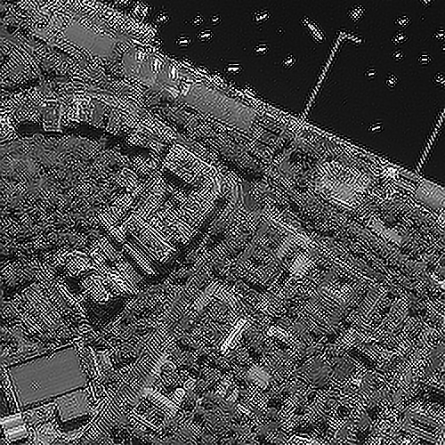 Figure 4
 Figure 5
 Figure 6
 Figure 7
 Figure 8
 Figure 9
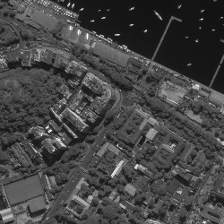 Figure 10
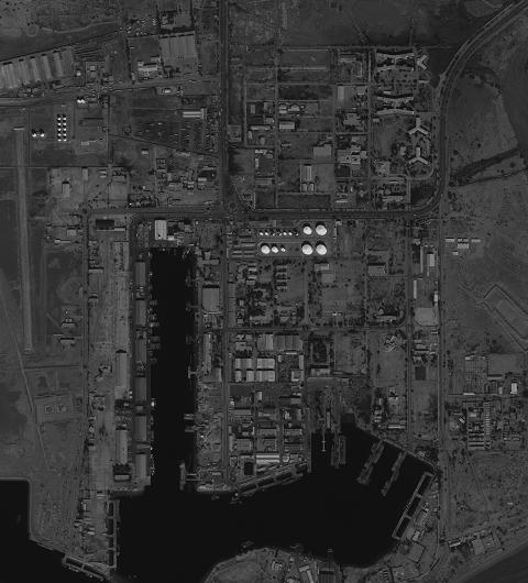 Figure 11
 Figure 12
 Figure 13
 Figure 14
 Figure 15
 Figure 16
 Figure 17
 Figure 18
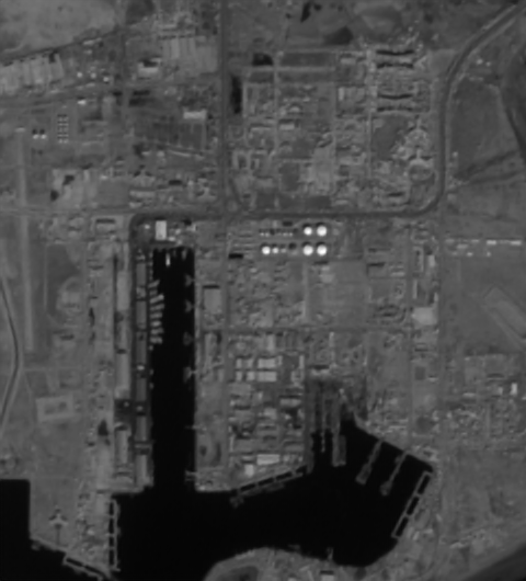 Figure 19
 Figure 20
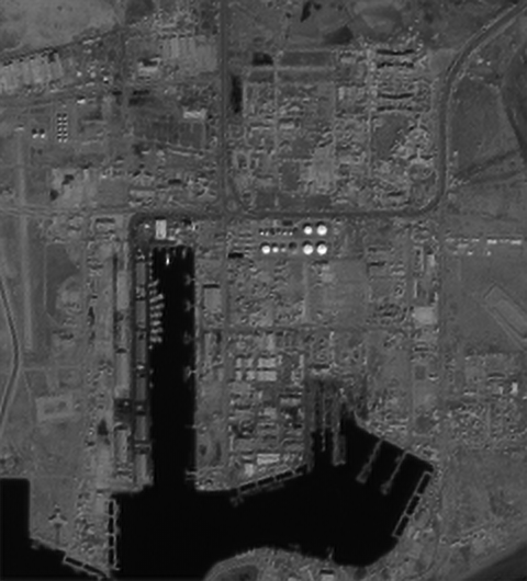 Figure 21
 Figure 22
 Figure 23
 Figure 24
 Figure 25
 Figure 26
 Figure 27
 Figure 28
 Figure 29
 Figure 30
 Figure 31
 Figure 32
 Figure 33
 Figure 34
 Figure 35
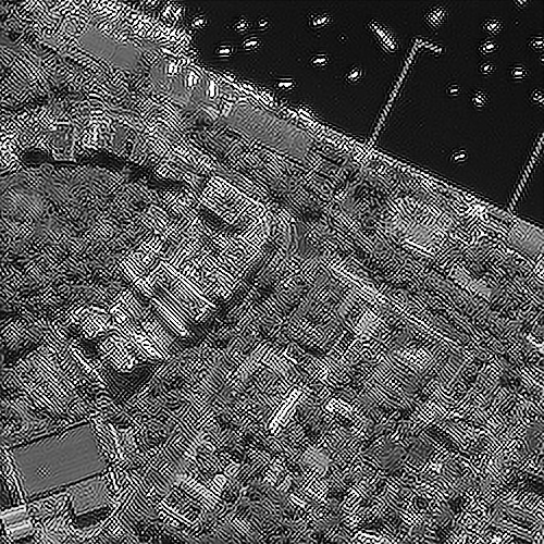 Figure 36
 Figure 37
 Figure 38
 Figure 39
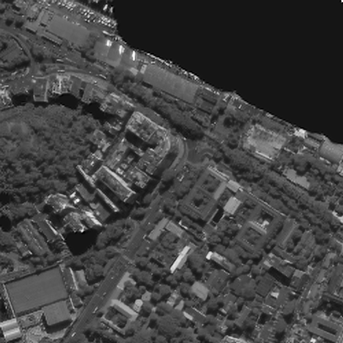 Figure 40
| Dataset | No. of patches in | No. of patches in | LR patch size | HR patch size |
| DIV2K | 12800 | 1600 | 112112 | 224224 |
| Sentinel | 4825 | 535 | 112112 | 224224 |
| Artificially-degraded (AD) satellite images | Real satellite (RS) images | ||||||||||||||||||||
| SRR method | FSRCNN [4] | SRResNet [7] | FSRCNN [4] | SRResNet [7] | |||||||||||||||||
| Downsampling of | PSNR | SSIM | UIQI | VIF | KFS | PSNR | SSIM | UIQI | VIF | KFS | PSNR | SSIM | UIQI | VIF | KFS | PSNR | SSIM | UIQI | VIF | KFS | |
| DIV2K | NN | 31.95 | 0.915 | 0.891 | 0.545 | 12.92 | 30.81 | 0.905 | 0.879 | 0.523 | 12.708 | 16.79 | 0.454 | 0.268 | 0.122 | 2.638 | 17.29 | 0.439 | 0.263 | 0.117 | 2.64 |
| Bilinear | 22.26 | 0.679 | 0.652 | 0.351 | 7.669 | 22.03 | 0.67 | 0.643 | 0.35 | 7.747 | 16.83 | 0.454 | 0.292 | 0.125 | 2.768 | 16.77 | 0.457 | 0.292 | 0.124 | 2.762 | |
| Bicubic | 26.61 | 0.819 | 0.792 | 0.435 | 10.209 | 26.84 | 0.82 | 0.794 | 0.44 | 10.375 | 16.44 | 0.433 | 0.262 | 0.109 | 2.61 | 16.97 | 0.465 | 0.287 | 0.124 | 2.705 | |
| Lanczos | 28 | 0.844 | 0.818 | 0.454 | 11.093 | 28.57 | 0.854 | 0.829 | 0.466 | 11.364 | 16.9 | 0.459 | 0.283 | 0.126 | 2.664 | 16.62 | 0.47 | 0.274 | 0.117 | 2.661 | |
| Lanczos-B | 11.02 | 0.175 | 0.168 | 0.118 | 3.591 | 10.98 | 0.167 | 0.162 | 0.11 | 3.514 | 15.32 | 0.313 | 0.21 | 0.098 | 2.817 | 15.45 | 0.336 | 0.218 | 0.099 | 2.819 | |
| Lanczos-N | 28.6 | 0.866 | 0.836 | 0.473 | 11.429 | 28.14 | 0.869 | 0.836 | 0.47 | 11.256 | 16.91 | 0.456 | 0.271 | 0.124 | 2.624 | 17.74 | 0.479 | 0.271 | 0.122 | 2.634 | |
| Lanczos-BN | 19.97 | 0.676 | 0.624 | 0.337 | 5.94 | 18.35 | 0.583 | 0.543 | 0.299 | 5.451 | 16.49 | 0.434 | 0.257 | 0.117 | 2.659 | 16.47 | 0.46 | 0.263 | 0.118 | 2.689 | |
| Mixed | 30.16 | 0.885 | 0.858 | 0.481 | 11.504 | 28.5 | 0.856 | 0.829 | 0.456 | 11.729 | 16.84 | 0.453 | 0.289 | 0.126 | 2.717 | 16.32 | 0.476 | 0.29 | 0.126 | 2.737 | |
| Sentinel-2 | NN | 31.64 | 0.91 | 0.88 | 0.531 | 12.794 | 31.59 | 0.908 | 0.875 | 0.527 | 12.43 | 16.88 | 0.438 | 0.242 | 0.11 | 2.553 | 16.08 | 0.441 | 0.254 | 0.11 | 2.591 |
| Bilinear | 23.01 | 0.701 | 0.676 | 0.358 | 7.467 | 23.01 | 0.669 | 0.632 | 0.308 | 6.378 | 17.12 | 0.491 | 0.292 | 0.124 | 2.772 | 16.9 | 0.507 | 0.279 | 0.109 | 2.682 | |
| Bicubic | 27.82 | 0.837 | 0.804 | 0.426 | 10.636 | 27.97 | 0.844 | 0.797 | 0.435 | 9.702 | 16.38 | 0.502 | 0.287 | 0.126 | 2.769 | 16.93 | 0.458 | 0.227 | 0.079 | 2.568 | |
| Lanczos | 28.41 | 0.85 | 0.823 | 0.459 | 11.04 | 26.18 | 0.833 | 0.807 | 0.445 | 11.04 | 16.93 | 0.49 | 0.285 | 0.126 | 2.686 | 15.52 | 0.482 | 0.254 | 0.105 | 2.593 | |
| Lanczos-B | 12.2 | 0.216 | 0.207 | 0.134 | 3.722 | 12.21 | 0.221 | 0.202 | 0.073 | 2.54 | 15.63 | 0.337 | 0.216 | 0.099 | 2.806 | 15.49 | 0.4 | 0.225 | 0.098 | 2.769 | |
| Lanczos-N | 28.67 | 0.865 | 0.839 | 0.474 | 11.348 | 28.68 | 0.868 | 0.842 | 0.48 | 11.557 | 16.88 | 0.487 | 0.275 | 0.127 | 2.652 | 17.35 | 0.528 | 0.265 | 0.122 | 2.664 | |
| Lanczos-BN | 20.7 | 0.702 | 0.663 | 0.342 | 6.014 | 18.79 | 0.6 | 0.553 | 0.281 | 5.203 | 16.53 | 0.455 | 0.269 | 0.12 | 2.718 | 17.02 | 0.515 | 0.261 | 0.114 | 2.71 | |
| Mixed | 28.23 | 0.847 | 0.817 | 0.431 | 10.576 | 20.83 | 0.843 | 0.805 | 0.45 | 9.555 | 16.99 | 0.461 | 0.291 | 0.126 | 2.778 | 13.47 | 0.46 | 0.237 | 0.084 | 2.563 | |
Peer Reviews
No public reviews on file for this paper yet. If you reviewed it on a platform where reviews are public (OpenReview, ICLR, NeurIPS, ICML), you can paste yours below so the community can read it here.
Videos
No videos yet. Explain this paper in a talk, walkthrough, or lecture? Add one.
On training deep networks for satellite image super-resolution
Abstract
The capabilities of super-resolution reconstruction (SRR)—techniques for enhancing image spatial resolution—have been recently improved significantly by the use of deep convolutional neural networks. Commonly, such networks are learned using huge training sets composed of original images alongside their low-resolution counterparts, obtained with bicubic downsampling. In this paper, we investigate how the SRR performance is influenced by the way such low-resolution training data are obtained, which has not been explored up to date. Our extensive experimental study indicates that the training data characteristics have a large impact on the reconstruction accuracy, and the widely-adopted approach is not the most effective for dealing with satellite images. Overall, we argue that developing better training data preparation routines may be pivotal in making SRR suitable for real-world applications.
**Index Terms— ** Super-resolution reconstruction, deep learning, convolutional neural networks, satellite imaging
1 Introduction
Super-resolution reconstruction (SRR) is aimed at generating a high-resolution (HR) image from a low-resolution (LR) observation (a single image or multiple images) [10]. SRR is a deeply explored research topic of considerable practical potential, as developing effective SRR techniques may allow for overcoming the spatial resolution limitations of the imaging sensors, which is a common problem in remote sensing.
1.1 Related work
Existing single-image SRR methods can be categorized into: (i) frequency-domain techniques [2], (ii) reconstruction-based methods which exploit prior knowledge on the object appearance [11], and (iii) algorithms that learn the mapping between LR and HR [12]. Recently, we have witnessed a breakthrough in the learning-based single-image SRR, attributed to the use of deep convolutional neural networks (CNNs). Deep learning SRR originates from sparse coding [12], aimed at creating a dictionary of LR patches, associated with their HR counterparts. The reconstruction consists in exploiting that dictionary for converting each LR patch from the input image into HR.
Super-resolution CNN (SRCNN) [3], followed by its faster version (FSRCNN) [4], was proposed for learning the LR-to-HR mapping from a number of LR–HR image pairs. Despite relatively simple architecture, SRCNN outperforms the state-of-the-art example-based methods. In [8], SRCNN was trained with Sentinel-2 images, which according to the authors improved its capacities of enhancing satellite data. Certain limitations of SRCNN were addressed with a very deep super-resolution network [6], trained relying on fast residual learning. The domain expertise was exploited in a sparse coding network [9], achieving high training speed and model compactness. Recently, generative adversarial networks are being actively explored for SRR [7]. They are composed of a generator (ResNet in [7]), trained to perform SRR, and a discriminator which tries to distinguish the ResNet reconstruction outcomes from real HR images.
1.2 Contribution
Deep CNNs for SRR are trained from a dataset of corresponding LR–HR patches. As deep networks commonly require huge amounts of training data, LR images are obtained by subjecting the original HR images to a degradation procedure based on an assumed imaging model. In most works [3, 7, 8], bicubic downsampling is applied to transform HR into LR, and in some cases [4], the training set () is additionally augmented with translation, rotation, and scaling. However, it has not been analyzed whether and how (including the degradation procedure) influences the reconstruction accuracy.
In this paper, our contribution consists in addressing the aforementioned research gap. We investigate the influence of , used for training a CNN, on the reconstruction performance. We trained two different CNNs (Section 2) with natural images from the DIV2K single-image SRR benchmark, and with Sentinel-2 images. The trained CNNs are tested in two settings: for reconstructing artificially-degraded satellite images (original images are treated as reference HR data), as well as in a real-world scenario—for original Sentinel-2 images, matched with SPOT and Digital Globe WorldView-4 images of the same region. The results of our extensive experiments (reported in Section 3) indicate that the degradation procedure used for creating plays a pivotal role here. Not only does it have a larger impact on the SRR performance than the domain of images exploited for training (natural vs. satellite), but it is also more important than the choice of the CNN architecture.
2 Deep learning for super-resolution
In this work, we exploit two CNNs of different complexity, namely: FSRCNN [4], which is a relatively shallow CNN, and a much deeper residual network (SRResNet [7]), to investigate their behavior in different training scenarios.
Figure 1 shows the architecture of FSRCNN [4]—the network is composed of five major parts aimed at: (i) feature extraction, realized by the first convolutional layer (denoted as Conv) with kernels of size , (ii) shrinking, performed using kernels () to reduce the number of features (from to ), (iii) non-linear mapping using multiple () convolutional layers with kernels (), (iv) expansion which inverses the shrinking and increases the dimensionality of the feature vectors from back to , and (v) deconvolution which produces the reconstructed HR image. FSRCNN can be trained faster than SRCNN and it offers real-time performance after training [3, 4].
The SRResNet [7] architecture (Fig. 2) benefits from the residual connections between the layers [5]. The residual blocks (RBs) are the groups of layers stacked together with the input of the block added to the output of the final layer contained in this block. In SRResNet, each block encompasses two convolutional layers, each followed by a batch normalization (BN) layer that neutralizes the internal co-variate shift. The upsampling blocks (UBs) allow for image enlargement by pixel shuffling (PS) layers that increase the resolution of the features. The number of both RBs and UBs is variable—by increasing the number of RBs, the network may model a better mapping, whereas by changing the number of UBs, we may tune its scaling factor. However, by adding more blocks, the architecture of the network becomes increasingly complex, which makes it harder to train.
3 Experimental study
We trained FSRCNN and SRResNet using natural images from the DIV2K dataset111Available at https://data.vision.ee.ethz.ch/cvl/DIV2K, and Sentinel-2 images. From these images, the patches were extracted randomly to create and validation set (), as specified in Table 1. LR images were obtained from HR ones using different downsampling techniques: nearest neighbor (NN), bilinear, bicubic, and Lanczos. We also created a mixed set—the downsampling technique was randomly selected for each image. For Lanczos, we additionally applied Gaussian blur with (Lanczos-B), Gaussian noise with (Lanczos-N), and both blur and noise with (Lanczos-BN). Examples of patches in are shown in Fig. 3. We used Python with Keras to implement the CNNs. The experiments were run on an Intel i9 4 GHz computer with 64 GB RAM, and two RTX 2080 8 GB GPUs. We used ADAM optimizer with learning rate of . The optimization stops, if after 50 epochs the accuracy over does not increase.
After training, the nets were tested using two kinds of test sets (): (i) artificially-degraded (AD) images—10 HR images of size pixels, bicubically downsampled to pixels, and (ii) real satellite (RS) images acquired at different resolution—we used three Sentinel-2 scenes as LR, two of which are matched with SPOT images and one is matched with Digital Globe WorldView-4 image. We evaluate the reconstruction accuracy relying on peak signal-to-noise ratio (PSNR), structural similarity index (SSIM), visual information fidelity (VIF), universal image quality index (UIQI), and keypoint features similarity (KFS) [1]. For all these metrics, higher values indicate higher similarity between the reconstruction outcome and the reference image.
In Table 2, we show the reconstruction accuracy obtained with FSRCNN and SRResNet trained using different ’s. We highlight PSNR and SSIM scores (in gray) for AD after training with bicubically downsampled , as this is the scenario most often reported in the literature. From these scores, SRResNet is slightly better than FSRCNN, and using satellite data for training appears to be beneficial. However, from all the scores, it is clear that the degradation procedure is more significant than both the type of images in and the network architecture. Actually, the nets trained with ’s based on NN perform in the best way, which can also be assessed qualitatively from Fig. 4. If is blurred (Lanczos-B), then the image sharpening is too strong, resulting in many high-frequency artifacts. A surprising outcome can be observed for SRResNet (Bicubic, Sentinel)—the details in the sea area are lost after reconstruction, but the land area is reliably restored.
For RS images, it is not clear from the reported metrics (Table 2), which is the best. The values are much lower than for AD, as the HR images used for reference are acquired using a different sensor, so even if an image is well reconstructed, it is substantially different from HR. From Fig. 5, it can be seen that NN downsampling (best for AD) results in a blurry outcome. Interestingly, Lanczos-B (very poor for AD), delivers better results in this case (and it is consistently picked by the KFS metric—the similarity to HR in the domain of the detected keypoints is the highest here). Similarly to AD, severe artifacts in the sea area can be observed for SRResNet trained with some ’s (Mixed and NN, for Sentinel). In our opinion, visually most plausible results are obtained using bilinear downsampling (for both Sentinel and DIV2K), which is also reflected with the highest UIQI scores in Table 2.
4 Conclusions
In this paper, we reported our experimental study on preparing the data to train deep CNNs for satellite image SRR. The results indicate that the degradation procedure used to generate the training data has a tremendous impact on the SRR performance, which is usually neglected in the literature. Furthermore, it is worth noting that much deeper architecture of SRResNet does not seem to outperform a relatively simple FSRCNN, when appropriate is used.
Currently, we are exploring how to combine different degradation procedures, including data augmentation techniques, to create training sets which better reflect the actual imaging conditions. We expect that this will allow deep CNNs to increase their performance for real satellite images.
The reference list from the paper itself. Each links out to its DOI / PubMed record.
- 1[1] P. Benecki, M. Kawulok, D. Kostrzewa, and L. Skonieczny, “Evaluating super-resolution reconstruction of satellite images,” Acta Astronautica , vol. 153, pp. 15–25, 2018.
- 2[2] H. Demirel and G. Anbarjafari, “Discrete wavelet transform-based satellite image resolution enhancement,” IEEE TGRS , vol. 49, no. 6, pp. 1997–2004, 2011.
- 3[3] C. Dong, C. C. Loy, K. He, and X. Tang, “Image super-resolution using deep convolutional networks,” IEEE TPAMI , vol. 38, no. 2, pp. 295–307, 2016.
- 4[4] C. Dong, C. C. Loy, and X. Tang, “Accelerating the super-resolution convolutional neural network,” in Proc. ECCV . Springer, 2016, pp. 391–407.
- 5[5] K. He, X. Zhang, S. Ren, and J. Sun, “Deep residual learning for image recognition,” in Proc. IEEE CVPR , 2016, pp. 770–778.
- 6[6] J. Kim, J. Kwon Lee, and K. Mu Lee, “Accurate image super-resolution using very deep convolutional networks,” in Proc. IEEE CVPR , 2016, pp. 1646–1654.
- 7[7] C. Ledig, L. Theis, F. Huszár et al. , “Photo-realistic single image super-resolution using a generative adversarial network.” in Proc. CVPR , vol. 2, no. 3, 2017, p. 4.
- 8[8] L. Liebel and M. Körner, “Single-image super resolution for multispectral remote sensing data using CN Ns,” in Proc. ISPRSC , 2016, pp. 883–890.