Comparison between Variational Monte Carlo and Shell Model Calculations of Neutrinoless Double Beta Decay Matrix Elements in Light Nuclei
X.B. Wang, A.C. Hayes, J. Carlson, G.X. Dong, E. Mereghetti, S., Pastore, R.B. Wiringa
TL;DR
This paper compares variational Monte Carlo and shell model methods for calculating neutrinoless double beta decay matrix elements in light nuclei, highlighting the importance of both long-range and short-range correlations for accuracy.
Contribution
It provides a detailed benchmark comparison between VMC and shell model calculations, assessing uncertainties and the effects of model choices in light nuclei.
Findings
VMC matrix elements show small variational uncertainties.
Shell model results depend on model space and correlation treatments.
Accurate decay matrix elements require proper inclusion of correlations.
Abstract
Benchmark comparisons between many-body methods are performed to assess the ingredients necessary for an accurate calculation of neutrinoless double beta decay matrix elements. Shell model and variational Monte Carlo (VMC) calculations are carried out for and nuclei. Different variational wavefunctions are used to evaluate the uncertainties in the {\it ab initio} calculations, finding fairly small differences between the VMC double beta decay matrix elements. For shell model calculations, the role of model space truncation, radial wavefunction choices, and short-range correlation are investigated and all found to be important. Based on the detailed comparisons between the VMC and shell model approaches, we conclude that accurate descriptions of neutrinoless double beta decay matrix elements require a proper treatment of both long-range and short-range correlations.
Click any figure to enlarge with its caption.
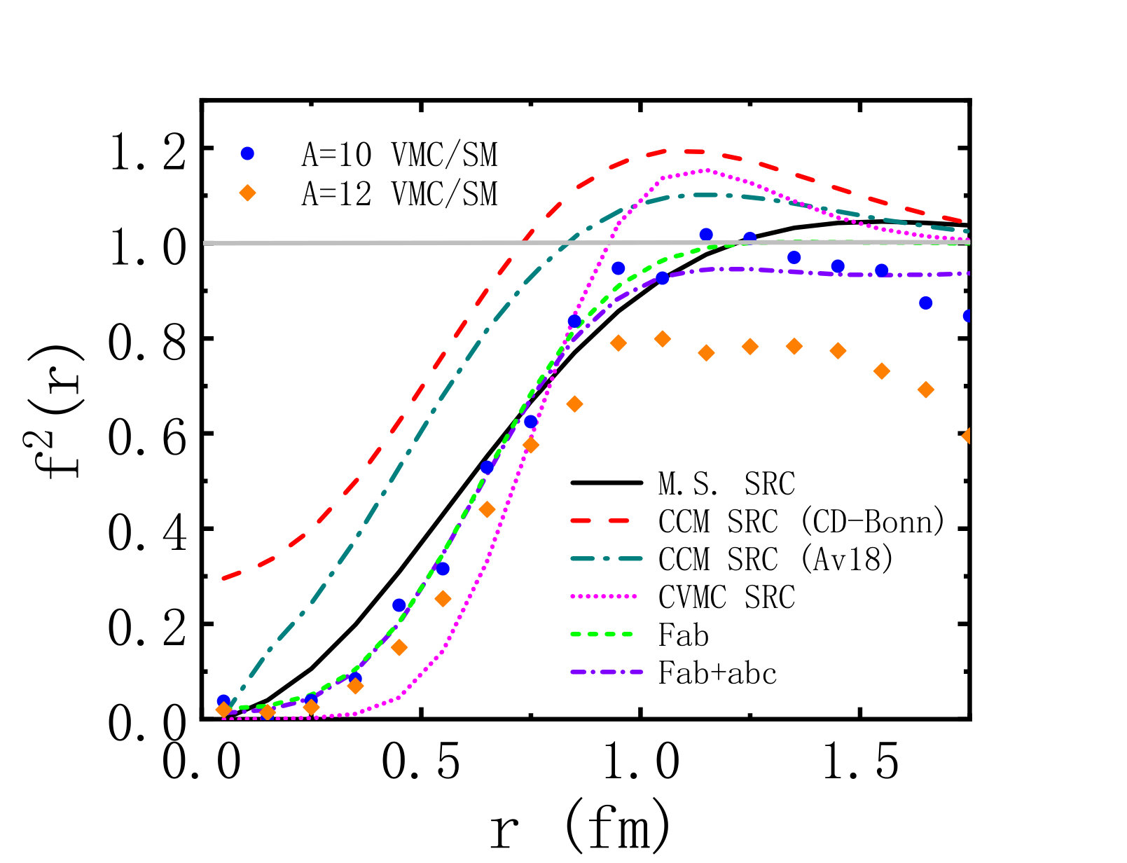 Figure 1
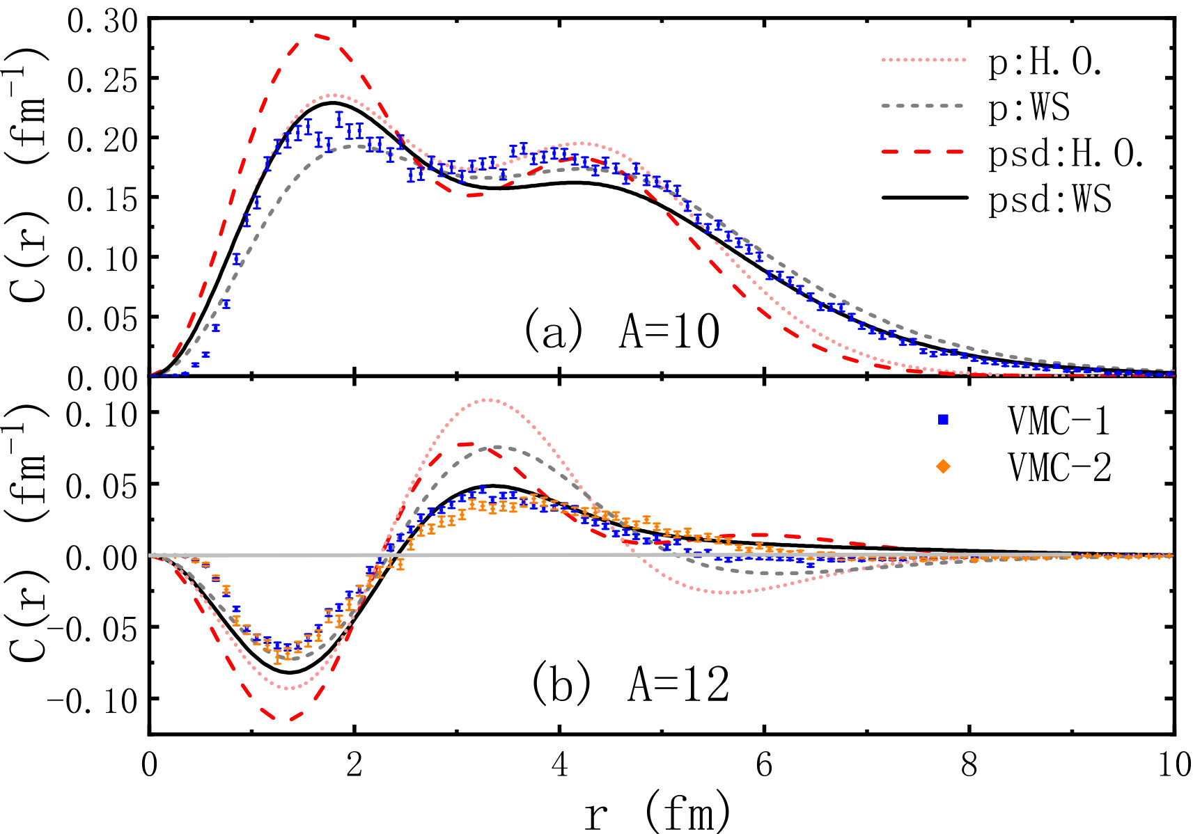 Figure 2
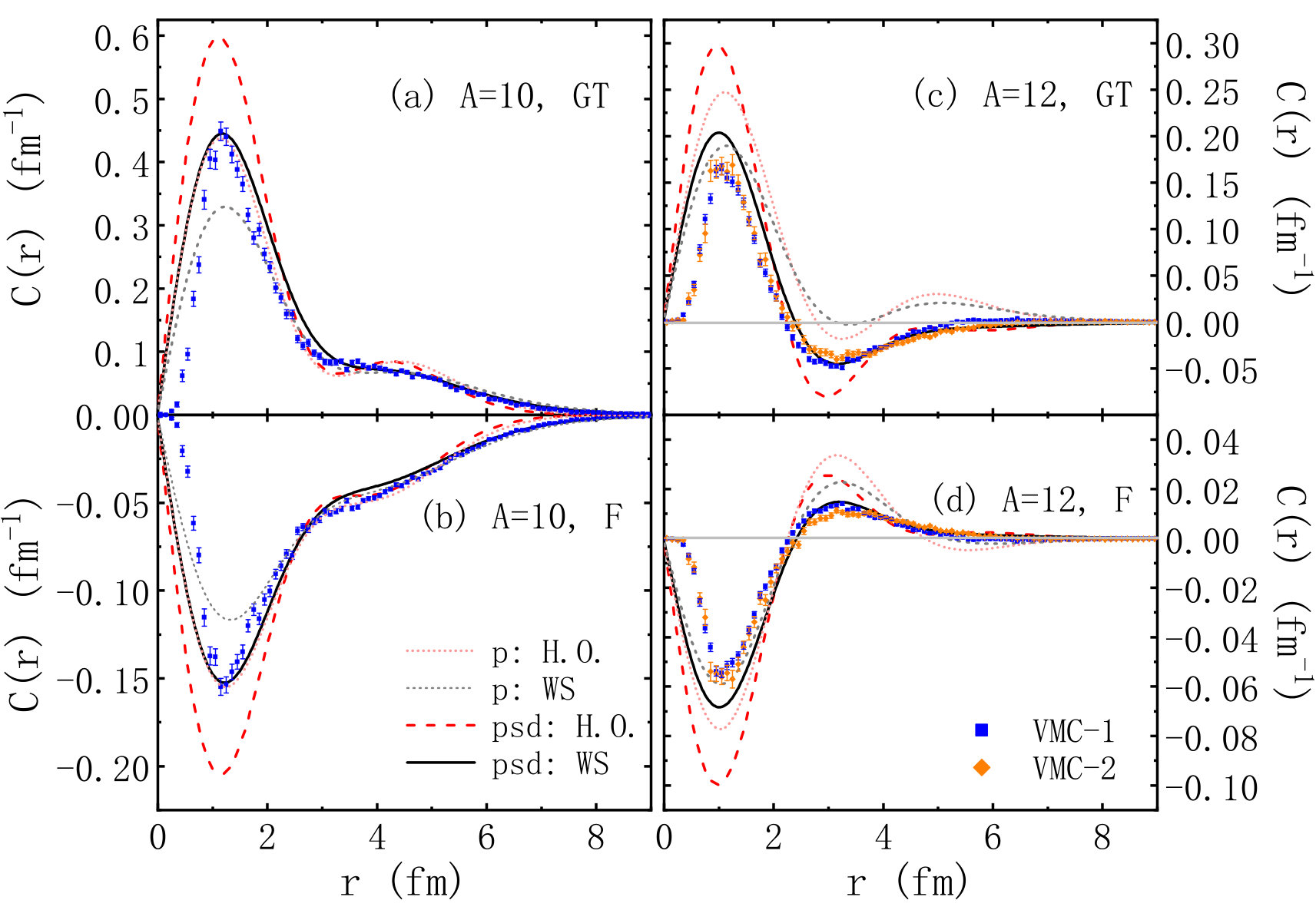 Figure 3
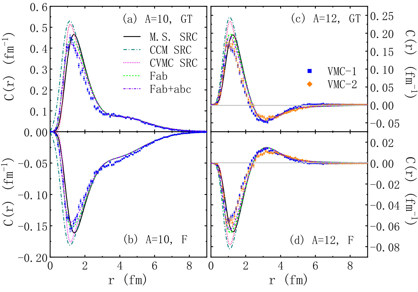 Figure 4
| 10Be()C() | 12Be()C() | |||
| F | GT | F | GT | |
| VMC-1 | -1.001(40) | 2.273(91) | -0.100(4) | 0.257(10) |
| VMC-2 | — | — | -0.113(5) | 0.274(11) |
| SM(w/o SRC, ) | -1.127 | 2.616 | -0.183 | 1.228 |
| SM(w/o SRC, ) | -0.980 | 2.269 | -0.147 | 1.023 |
| SM(w/o SRC, ) | -1.274 | 3.228 | -0.271 | 0.431 |
| SM(w/o SRC, ) | -1.100 | 2.783 | -0.198 | 0.570 |
| SM(M.S. SRC, ) | -0.967 | 2.381 | -0.122 | 0.342 |
| SM(CCM SRC, ) | -1.069 | 2.683 | -0.175 | 0.499 |
| SM(CVMC SRC, ) | -0.992 | 2.457 | -0.141 | 0.398 |
| SM(Fab, ) | -0.988 | 2.449 | -0.138 | 0.388 |
| SM(Fab+abc, ) | -0.957 | 2.362 | -0.128 | 0.361 |
Peer Reviews
No public reviews on file for this paper yet. If you reviewed it on a platform where reviews are public (OpenReview, ICLR, NeurIPS, ICML), you can paste yours below so the community can read it here.
Videos
No videos yet. Explain this paper in a talk, walkthrough, or lecture? Add one.
Comparison between Variational Monte Carlo and Shell Model Calculations of Neutrinoless Double Beta Decay Matrix Elements in Light Nuclei
X.B. Wanga, A.C. Hayesb, J. Carlsonb, G.X. Donga, E. Mereghettib, S. Pastorec and R.B. Wiringad
aSchool of Science, Huzhou University, Huzhou 313000, ChinabTheoretical Division, Los Alamos National Laboratory, Los Alamos, NM 87545, USA cDepartment of Physics, Washington University in St. Louis, MO 63130, USAdPhysics Division, Argonne National Laboratory, Argonne, IL 60439, USA
Abstract
Benchmark comparisons between many-body methods are performed to assess the ingredients necessary for an accurate calculation of neutrinoless double beta decay matrix elements. Shell model and variational Monte Carlo (VMC) calculations are carried out for and nuclei. Different variational wavefunctions are used to evaluate the uncertainties in the ab initio calculations, finding fairly small differences between the VMC double beta decay matrix elements. For shell model calculations, the role of model space truncation, radial wavefunction choices, and short-range correlation are investigated and all found to be important. Based on the detailed comparisons between the VMC and shell model approaches, we conclude that accurate descriptions of neutrinoless double beta decay matrix elements require a proper treatment of both long-range and short-range correlations.
I Introduction
Neutrinoless double beta decay () is a process in which two neutrons in a nucleus decay into two protons, with the emission of two electrons and no neutrinos, thus violating lepton number () by two units. The observation of would imply that neutrinos are Majorana particles Schechter and Valle (1982), shed light on the mechanism of neutrino mass generation, and give insight into leptogenesis scenarios for the generation of the matter-antimatter asymmetry in the universe Davidson et al. (2008). For these reasons, is the subject of intense experimental research programs Gando et al. (2013); Agostini et al. (2013); Albert et al. (2014); Andringa et al. (2016); Gando et al. (2016); Elliott et al. (2017); Agostini et al. (2017); Aalseth et al. (2018); Albert et al. (2018); Alduino et al. (2018); Agostini et al. (2018); Azzolini et al. (2018). Current experimental limits are already very stringent, constraining the half-lives of 76Ge, 130Te and 136Xe to be larger than yr Agostini et al. (2018), yr Azzolini et al. (2018) and yr Gando et al. (2016), respectively. The next-generation ton-scale experiments will improve these limits by one or two orders of magnitude.
rates depend not only on nuclear properties, but also on unknown fundamental lepton number violating (LNV) parameters, such as the Majorana masses of light neutrinos. Extracting the values of these parameters from experiments requires the evaluation of nuclear matrix elements (NMEs) of transition operators. Isotopes of experimental interest for 0 searches, e.g. 48Ca, 76Ge, 82Se, 124Sn, 128Te, 130Te and 136Xe, are medium and heavy open-shell nuclei with very complex nuclear structure. In addition, for these nuclei, one is forced by current computational limitations to utilize approximate methods to solve the nuclear many-body problem, and to work in a truncated model spaces where correlations and many-body terms in both the nuclear interactions and currents may be insufficient or neglected. Consequently, different theoretical models can give systematically different results. For example, the nuclear matrix elements of 48Ca have been calculated using the shell model Menendez et al. (2009); Sen’kov and Horoi (2013); Kwiatkowski et al. (2014); Iwata et al. (2016), energy density functionals López Vaquero et al. (2013), the quasiparticle random-phase approximation (QRPA) Šimkovic et al. (2013), and the interacting boson model (IBM) Barea et al. (2015), leading to results that differ by a factor of two or three. Similar variations are observed for other candidates Engel and Menéndez (2017).
Recently, a set of ab initio variational Monte Carlo (VMC) calculations of 0 decay matrix elements in nuclei has been reported by some of the present authors Pastore et al. (2018a). Within the ab initio VMC framework, the many-body problem is solved for nuclei up to , with a nuclear Hamiltonian consisting of two- and three-body interactions, namely the Argonne- (AV18) and Illinois- (IL7), respectively, and associated electroweak many-body currents. While the 0 transitions studied in Ref. Pastore et al. (2018a) are not directly relevant from an experimental point of view because the masses studied are too low, they provide a useful reference for more approximated nuclear methods. The ab initio framework used in the VMC approach accurately explains, qualitatively and quantitatively, the observed electroweak properties of light nuclei Carlson et al. (2015); Carlson and Schiavilla (1998); Bacca and Pastore (2014) over a broad range of momentum transfers, so that VMC results provide an important benchmark to test other many-body methods that can be extended to the heavy nuclei of experimental interest.
The goal of the present work is to benchmark shell model calculations of the relevant NMEs in light nuclei to the aforementioned VMC results. We wish to examine the model dependence and uncertainties involved in shell model approaches and to identify the degree of sophistication that needs to be included in such a calculational approach to . In general, shell model calculations involve a number of choices, including the size of the model space, the effective nucleon-nucleon interaction, the radial wave functions, and the short-range correlation (SRC) functions used. In the current work, we concentrate on nuclei of mass 10 and 12, and we examine the role played by these different nuclear structure inputs in determining the predicted NMEs.
The paper is organized as follows. In Section II, we present the two-body transition operators that mediate 0, and the shell model framework that is used to evaluate matrix elements of these operators. In Section III, we describe two sets of shell model calculations, and present a detailed analysis of uncertainties arising from different choices of the basis, radial functions, and SRC functions. Finally, in Section IV we discuss our results and present our conclusions.
II Neutrinoless double beta decay matrix elements
II.1 operators
We consider transitions induced by a Majorana mass term for light, left-handed neutrinos
[TABLE]
where , are the masses of the neutrino mass eigenstates, and are elements of the Pontecorvo-Maki-Nakagawa-Sato (PMNS) matrix. denotes the charge conjugation matrix. The operator in Eq. (1) arises from the Weinberg operator Weinberg (1979) after electroweak symmetry breaking, and the invariance of the Standard Model implies that , where is the Higgs vacuum expectation value and is the high-energy scale at which LNV arises. Eq. (1) is the first term in an expansion in , and, in general, will receive contributions from operators of dimension higher than five Pas et al. (2001, 1999); Prezeau et al. (2003); Lehman (2014); Graesser (2017); Cirigliano et al. (2017, 2018a). We limit ourselves to study nuclear matrix elements of the transition operator induced by , since its structure is rich enough to capture several features of non-standard mechanisms.
The transition operator, or “neutrino potential”, induced by has been derived in several papers Haxton and Stephenson (1984); Doi et al. (1985); Bilenky and Giunti (2015). In general, several operators contribute, with , and labeling the various components of the Fermi(F), Gamow-Teller(GT) and tensor(T) matrix elements of the vector (), axial-axial(AA), axial-pseudoscalar (AP), pseudoscalar-pseudoscalar (PP), and magnetic-magnetic (MM) operators. The leading operators are,
[TABLE]
where fm is the nuclear radius. The form of the neutrino potentials in coordinate space is given in Ref. Pastore et al. (2018a), where the corresponding potential in momentum space is also listed. The functions in Eq. (II.1) have different radial dependencies. In particular, and , which give the largest contributions to the NMEs, have a Coulombic dependence, up to corrections from the axial and vector form factors. The and components are induced by the induced pseudoscalar form factor, which is dominated by the pion pole, and thus have pion range. The components are generated by neutrinos coupling to the weak magnetic form factor, and have short-range. Finally, it was pointed out in Ref. Cirigliano et al. (2018b) that, in chiral effective field theory (EFT), the transition operator should be supplemented by a leading-order short-range component, in addition to , with unknown coefficient.
II.2 Variational Monte Carlo Method
In this work, VMC calculations used the same wave functions as constructed in Ref. Pastore et al. (2018a). Here, we summarize the calculations scheme adopted in that reference.
The evaluation of the matrix elements defined in Eq. (II.1) is carried out using VMC computational algorithms Carlson et al. (2015). The VMC wave function —where and are the spin-parity and isospin of the state—is constructed from products of two- and three-body correlation operators acting on an antisymmetric single-particle state of the appropriate quantum numbers. The correlation operators are designed to reflect the influence of the two- and three-body nuclear interactions at short distances, while appropriate boundary conditions are imposed at long range Wiringa (1991); Pudliner et al. (1997).
The has embedded variational parameters that are adjusted to minimize the expectation value
[TABLE]
which is evaluated by Metropolis Monte Carlo integration Metropolis et al. (1953). In the equation above, is the exact lowest eigenvalue of the nuclear Hamiltonian for the specified quantum numbers. The many-body Hamiltonian is given by
[TABLE]
where is the non-relativistic kinetic energy of nucleon and and are, respectively, the Argonne (AV18) Wiringa et al. (1995) two-body potential and the Illinois-7 (IL7) Pieper (2008) three-nucleon interaction. The AV18+IL7 model reproduces the experimental binding energies, charge radii, electroweak transitions and responses of – systems in numerically exact calculations based on Green’s function Monte Carlo (GFMC) methods Carlson and Schiavilla (1998); Bacca and Pastore (2014); Carlson et al. (2015); Pastore et al. (2018b).
A good variational wave function, that serves as the starting point of GFMC calculations, can be constructed with
[TABLE]
The Jastrow wave function is fully antisymmetric, translationally invariant, has the quantum numbers of the state of interest, and includes a product over pairs of a central correlation function that is small at short distances, peaks around 1 fm, and decays exponentially at long range Pieper and Wiringa (2001). The and are the two- and three-body correlation operators, and is a symmetrization operator. The two-body correlation operators Pieper and Wiringa (2001); Carlson et al. (2015) can be schematically written as
[TABLE]
where
[TABLE]
are the main static operators that appear in the two-nucleon potential and the are functions of the interparticle distance generated by the solution of a set of coupled differential equations containing the bare two-nucleon potential with asymptotically-confined boundary conditions Carlson et al. (2015).
The results presented below for nuclei use the VMC wave functions that serve as starting trial functions for the GFMC calculations in Ref. Carlson et al. (2015). For systems, we use both shell-model-like wave functions (denoted in the figures by “VMC-1”) and clusterized wave functions (denoted by “VMC-2”) which were originally used in the calculations reported in Ref. Nollett et al. (2001). The difference in these two types of variational wave functions is described below.
For nuclei, the Jastrow wave function of Eq. (5) is written as a sum over different -space symmetry combinations (where denotes the spatial symmetry Young diagram), each of which is an antisymmetric sum over partitions of nucleons into four s-shell nucleons and p-shell nucleons. For the shell-model-like wave function, each partition has a product over all pairs of a set of three central correlation functions, , where indicates both nucleons are in the s-shell, indicates both are in the p-shell, and that one is in each shell. Each of the has a different radial dependence with variational parameters to be optimized, but all p-shell particles are treated equally. Thus for a 12-body nucleus, there is a product of 6 , 32 , and 28 functions. In addition, the parametrization of the are allowed to be different for different components. For the 12C ground state we use 1S0[444] and 3P0[4431] spatial symmetry combinations, with coefficients determined in a energy diagonalization. For 12Be we use 1S0[4422] and 3P0[4332] combinations.
For the cluster-type wave functions, we allow for the formation of clusters in the p-shell by further partitioning the nucleons into subgroups and having multiple types of and . For the 12C 1S0[444] ground state there are two correlation functions, used according to whether both nucleons are in the same or different [4] clusters; effectively this builds a triple-alpha structure which is a major part of the 12C ground state. For the 12Be 1S0[4422] ground state there are three subgroups in the p-shell, effectively one alpha-like [4] cluster and two dineutron-like [2] clusters, with three and two correlation functions. These cluster-type wave functions are more sophisticated in construction, but the increase in the number of variational parameters to optimize is a burden, and only these highest spatial symmetry states have been used so far.
At present, the shell-model-like VMC-1 wave function for 12C with two spatial symmetry components gives a slightly better energy, while getting a charge radius closer to experiment than the cluster-like VMC-2 wave function with one spatial symmetry. The VMC-1 and VMC-2 wave functions for 12Be give comparable charge radii close to experiment, but the VMC-2 allows the neutron distribution to be more diffuse with a slightly better energy.
In what follows, we calculate matrix elements defined in Eq. (II.1), and their associated transition distributions in -space, , and -space, defined as
[TABLE]
where is the transition density associated with the transition operator .
II.3 NMEs within the shell model framework
Within the shell model, the matrix elements of the operators between many-body wave functions and can be calculated as a sum of products of two-body transition densities (TBTDs) between many-body states and antisymmetrized two-body matrix elements TBMEs between two-particle states, as
[TABLE]
Here the labels stands for the set of spherical quantum numbers describing the single nucleons making up the two-particle wave functions, and TBTD are matrix elements between the many-body wave functions given by,
[TABLE]
where is a two-particle creation operator of rank , as
[TABLE]
and .
III Calculations and discussions
We focus on the NMEs for the 10BeC and 12BeC transitions. The transition is between isobaric analog states, a situation that is never realized in experiments, but is nonetheless very useful for comparisons between models. In particular, as discussed below, the radial contributions to the A=10 matrix elements involve no nodes, in contrast to the A=12 case. As in Eq. (II.2), the radial contribution to the matrix elements is defined as , where .
Our shell model calculations are carried out using the code Oxbash Brown et al. . The PSDMWK shell model Hamiltonian Warburton and Brown (1992); Warburton et al. (1992) is used for the p- plus sd-shell () model space, with up to excitations. Lawson’s prescription is adopted for treating center of mass (C.M.) excitations Gloeckner and Lawson (1974). The same NMEs are also calculated by VMC, for which the Argonne two-nucleon potential plus Illinois-7 three-nucleon interaction are used. As discussed in Sec. II, two different sets of variational wave functions are used in the VMC calculations, namely the shell-model-like (VMC-1) and cluster-model-like (VMC-2).
III.1 The wave function normalization
We begin our study with a comparison of the wave function normalization densities
[TABLE]
displayed in Fig. 1. For the shell model calculations, we show the results for the shell and the more extended model space. In addition, we show shell model results using different choices of radial wave functions. The SRC functions are not included at this stage in the shell model wave functions.
Harmonic oscillator (H.O.) radial wave functions are commonly used in shell model calculations because H.O. basis have the advantage of a simple well-defined method of separating into center-of-mass and relative coordinates via Talmi-Brody-Moshinsky brackets Talmi (1952); Moshinsky (1959). However, H.O. wave functions exhibit the wrong asymptotic behavior at large interparticle distance, , which affects the calculation of NMEs. Thus, we examine the effect of using more realistic Woods-Saxon (WS) radial wave functions. In the case of WS wave functions, we take the -shell neutron and proton asymptotic wave function behavior to be determined by the corresponding experimental separation energies, while the unbound -shell particles are assumed to be bound by MeV. For the calculations of two-body matrix elements, we expand the WS wave functions into a H.O. basis, and then apply the Talmi-Moshinsky method.
As seen in both panels of Fig. 1, the extended shell model space results in a higher first (and lower second) peak in . Enlarging the model space introduces more correlations, making the nuclei more bound, and the wave functions more concentrated at short distances. The more realistic WS wave functions provide a better description at large . We note that the normalization of is unity for the A=10 isobaric analog transition, and zero for A=12 transition. The position of the nodes in the function has an important effect on the predictions for the NMEs.
As seen in panel (b) of Fig. 1, the first node appears at about 2 fm in both the shell model and VMC calculations. However, the smaller -shell model space has an extra node at around 5 fm, in contrast to the predictions of the larger model spaces. Neither VMC calculations predict this second node. Thus, we conclude that the size of the model space used is crucial for shell model estimates of NMEs.
III.2 The radial distribution of NMEs
We next consider the matrix elements of and , which have a simple Coulombic dependence and give the largest contributions to the NMEs. Detailed comparisons between the shell model and VMC calculations are shown in Fig. 2. Apart from the differences in magnitude and sign, the distribution for and have similar shapes. Because of the Coulombic dependence, the first peak of the distributions is much larger than the second peak, and the functions die off rapidly at large distance . As with the normalization functions, the shell model distributions from the larger model spaces show higher peaks than those from the smaller -shell model spaces, when the same radial wave functions are used. In general, the predicted shape of the functions is poor in the case of the small pure -shell calculations, and we again conclude that small shell model spaces are unlikely to provide accurate predictions. When a larger model space is used in combination with the more realistic WS wave functions, the shell model predictions are in reasonable agreement with the VMC results, except at very small fm.
III.3 The short-range correlation functions
Short-range correlations (SRC) arising from the repulsive hard core of the nucleon-nucleon interaction are absent from the radial wave functions used in shell model calculations. A standard approximate method for correcting this is to introduce a Jastrow-like correlation function, , of the form,
[TABLE]
The parameters have been determined using different assumptions. The Miller-Spencer (M.S.) SRC, modeled in 1976 Miller and Spencer (1976), is widely used in the literature. Newer sets of SRC have been obtained from correlated two-body wave function derived by the coupled-cluster method (CCM) Simkovic et al. (2009). More recently, through the study of paired density distributions in 16O and 40Ca by Cluster Variational Monte Carlo (CVMC) Pieper et al. (1992); Lonardoni et al. (2017), isospin dependent correlation functions have been suggested Cruz-Torres et al. (2018). Yet another set of correlation functions was obtained in Ref. Akmal and Pandharipande (1997) from nuclear matter variational calculations, and we also study the effects of using these functions. In Figs. 3 and 4, two-body correlation functions from Ref. Akmal and Pandharipande (1997) with and without three-body and higher order correlations are labeled with “Fab+abc” and “Fab”, respectively.
In Fig. 3, we show a comparison between the different Jastrow correlation functions which we used in calculating the shell model NMEs. This allows us to assess the sensitivity of our shell model results with respect to variations in the SRCs. The points in Fig. 3 denote the ratio of the normalization density , defined in Eq. (12), computed in the VMC and in the shell-model for A=10 and 12. This ratio might be regarded as a rough estimate of short-range dynamics present in VMC versus shell model calculations.
As seen in the figure, most of short-range correlations overshoot unit at intermediate distance, and exhibit a correlation “hole” at short distance. Such overshoot is needed to preserve the wave function normalizations, as has been studied in Ref. Engel et al. (2011). The Miller-Spencer SRC function peaks at about 1.5 fm, while more modern functions, CCM SRC and CVMC SRC, peak at 1.0 fm. The CVMC SRC exhibits a more pronounced peak and hole relative to the CCM SRC (A). As discussed in the next section, the difference in NME predictions obtained using the different SRC functions reflects a general uncertainty in the shell model calculations.
III.4 Results
In Fig. 4, shell model matrix elements using the different SRC functions are shown. In these calculations, shells with WS wave functions are used. As expected, the degree of suppression at small of the function is dependent on the SRC used. The resulting NMEs are given in Table. 1. The VMC calculations with the two different type of wave functions give very similar results. However, within a shell model framework, several important ingredients must be included for realistic predictions. These include the size of the model space, the choice of radial wave functions and the inclusion of realistic SRC functions.
For =10, the extension of shell model space results in larger (in absolute value) NMEs. For =12, the extension of the model space results in smaller matrix elements, because of the cancellations from contributions above and below the node in . The use of more realistic radial wave functions, WS versus HO, also reduces the predicted NMEs. The inclusion of a SRC function is important to further reduce the shell model predictions and to obtain realistic functions . In Ref. Kortelainen et al. (2007), it was reported that for 48Ca and 76Ge, a 30 to 40 reduction of NMEs arose from the inclusion of the M.S. SRC. In the present study of light nuclei, the M.S. SRC reduces the NMEs by about 20 . Among more modern SRC functions, respecting the preservation of wave-function normalization Engel et al. (2011), SRC fitted from CVMC also gives similar reduction of NMEs.
IV summary and conclusion
In the current study, we compare NMEs predictions in light nuclei from shell model calculations with VMC calculations. In all cases the bare operators are used. The VMC calculations agree well with numerically exact GMFC calculations, reproducing nuclear radii and electroweak distributions. In this sense, the VMC calculations act as a benchmark for comparison to other models.
We study two very different double beta-decay transitions, 10BeC and 12BeC. The most significant difference between these two transitions is that nuclear structure causes the radial contributions to the matrix elements in A=10 to be nodeless, whereas the same distributions for A=12 involve nodes and hence cancellations in the matrix elements.
We examine the role of various model-dependent choices that go into shell model calculations of matrix elements, including the the size of the model space, radial wave functions, and the SRC functions. The largest impact on the shell model predictions comes from the many-body correlations that are introduced by increasing the size of the model space. In both A=10 and A=12, the transition densities determining the matrix elements of from the larger shell model calculation come significantly closer to the predictions of the VMC calculations than do the predictions from the smaller shell model spaces.
The change in the absolute magnitude of the and matrix elements with increasing shell model space is different for A=10 and A=12. In both cases the magnitude of the peaks in the distribution increase. In the case of the nodeless A=10 function, this translates into an overall increase in the absolute magnitude of the matrix elements. In contrast, the change in the magnitude of the peaks, coupled with the shift in the position of the node, causes the A=12 cancellations from contributions above and below the node of C(r) to reduce (increase) the absolute magnitude of the () matrix element by a factor of 2 (1.4).
The use of more realistic WS radial wave functions, that take the separation energies of the transferred neutrons and protons into account, reduce the magnitudes of the NMEs because of the reduced overlap between the neutron and proton wave functions. By using the WS wave functions and increased model space, the long-range behavior of distribution is found to be in excellent agreement with the VMC predictions.
The SRC functions affect the contributions to the matrix elements at short distance (less than 1.5 fm). We have examined several different SRC functions. In general, the introduction of SRCs moves the shell model predictions closer to the VMC calculations, reducing the NMEs. The magnitude of this reduction is dependent on the SRC function used.
While the present calculations in light nuclei cannot be used to make definitive statements about the validity of shell model calculations in medium and heavy nuclei, they do suggest some trends. First, the use of H.O. radial wave functions will likely lead to an overestimate of matrix elements. Second, and perhaps more importantly, limited size model space calculations could affect the magnitude of the predicted matrix elements, particularly for calculations constrained to a single shell. Third, the inclusion of a SRC function is needed. The best choice for this function requires further study.
Acknowledgements.
We thank V. Cirigliano and W. Dekens for helpful discussions. X.B. Wang and G.X. Dong thank the support by National Natural Science Foundation of China under Grant Nos. U1732138, 11605054, 11505056, and 11847315, and especially thank the hospitality and financial support of Los Alamos National Laboratory. This research is also supported by the U.S. Department of Energy, Office of Science, Office of Nuclear Physics, under contracts DE-AC02-06CH11357 (R.B.W.), and DE-AC52-06NA25396 and the Los Alamos LDRD program. The work R.B.Wiringa has been supported by the Nuclear Computational Low-Energy Initiative (NUCLEI) SciDAC project. Computational resources have been provided by Los Alamos Open Supercomputing, and Argonne’s Laboratory Computing Resource Center.
The reference list from the paper itself. Each links out to its DOI / PubMed record.
- 1Schechter and Valle (1982) J. Schechter and J. W. F. Valle, Phys. Rev. D 25 , 2951 (1982) , [,289(1981)]. · doi ↗
- 2Davidson et al. (2008) S. Davidson, E. Nardi, and Y. Nir, Phys. Rept. 466 , 105 (2008) , ar Xiv:0802.2962 [hep-ph] . · doi ↗
- 3Gando et al. (2013) A. Gando et al. (Kam LAND-Zen), Phys. Rev. Lett. 110 , 062502 (2013) , ar Xiv:1211.3863 [hep-ex] . · doi ↗
- 4Agostini et al. (2013) M. Agostini et al. (GERDA), Phys. Rev. Lett. 111 , 122503 (2013) , ar Xiv:1307.4720 [nucl-ex] . · doi ↗
- 5Albert et al. (2014) J. B. Albert et al. (EXO-200), Nature 510 , 229 (2014) , ar Xiv:1402.6956 [nucl-ex] . · doi ↗
- 6Andringa et al. (2016) S. Andringa et al. (SNO+), Adv. High Energy Phys. 2016 , 6194250 (2016) , ar Xiv:1508.05759 [physics.ins-det] . · doi ↗
- 7Gando et al. (2016) A. Gando et al. (Kam LAND-Zen), Phys. Rev. Lett. 117 , 082503 (2016) , [Addendum: Phys. Rev. Lett.117,no.10,109903(2016)], ar Xiv:1605.02889 [hep-ex] . · doi ↗
- 8Elliott et al. (2017) S. R. Elliott et al. , Proceedings, 27th International Conference on Neutrino Physics and Astrophysics (Neutrino 2016): London, United Kingdom, July 4-9, 2016 , J. Phys. Conf. Ser. 888 , 012035 (2017) , ar Xiv:1610.01210 [nucl-ex] . · doi ↗