Quasinormal modes of three-dimensional rotating Ho\v{r}ava AdS black hole and the approach to thermal equilibrium
Ram\'on B\'ecar, P. A. Gonz\'alez, Eleftherios Papantonopoulos and, Yerko V\'asquez

TL;DR
This paper calculates the quasinormal modes of a scalar field in a rotating three-dimensional Hořava AdS black hole, revealing stability and insights into the system's thermalization process under Lorentz invariance breaking.
Contribution
It provides the first analysis of quasinormal modes in a rotating Hořava AdS black hole, exploring the effects of Lorentz invariance violation on stability and thermalization.
Findings
Scalar field propagation is stable in this background.
Different solutions reach thermal equilibrium at different times.
Lorentz invariance breaking influences QNM characteristics.
Abstract
We compute the quasinormal modes (QNMs) of a massive scalar field in the background of a rotating three-dimensional Ho\v{r}ava AdS black hole, and we analyze the effect of the breaking of the Lorentz invariance on the QNMs. Imposing on the horizon that there are only ingoing waves and at infinity the Dirichlet boundary conditions and the Neumann boundary condition, we calculate the oscillatory and the decay modes of the QNMs. We find that the propagation of the scalar field is stable in this background and employing the holographic principle we find the different times of the perturbed system to reach thermal equilibrium for the various branches of solutions.
Click any figure to enlarge with its caption.
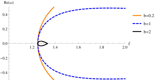 Figure 1
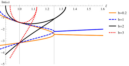 Figure 2
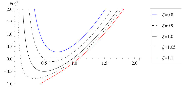 Figure 3
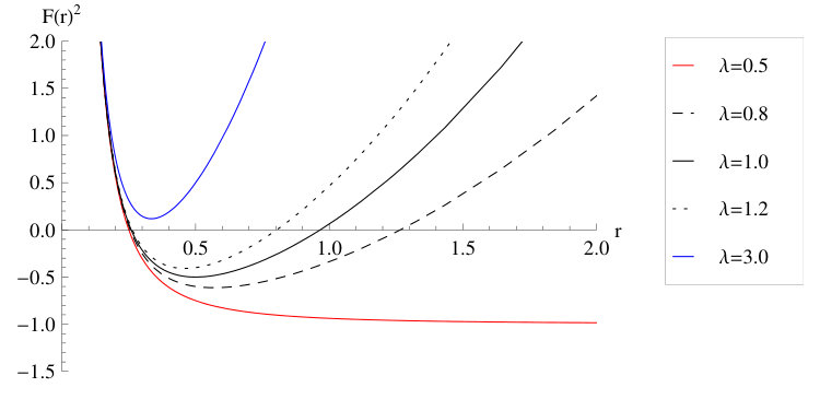 Figure 4
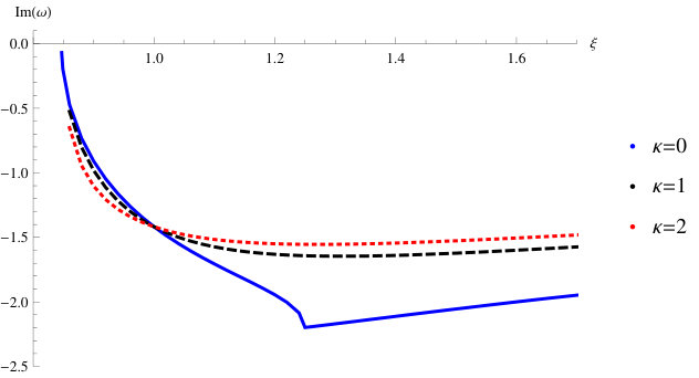 Figure 5
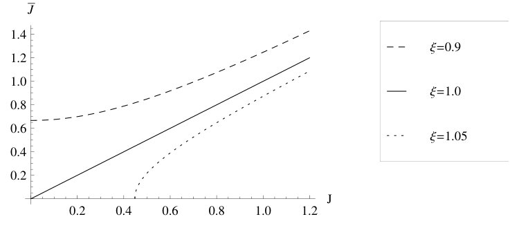 Figure 6
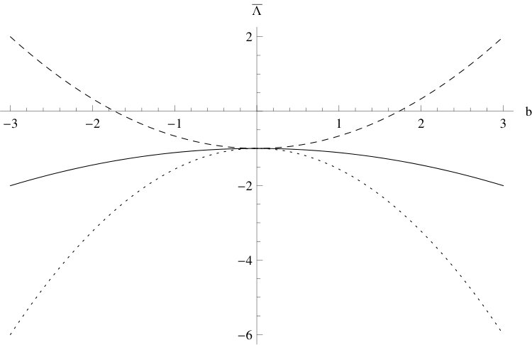 Figure 7
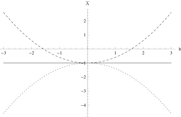 Figure 8
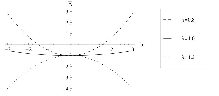 Figure 9
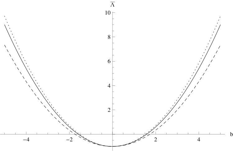 Figure 10
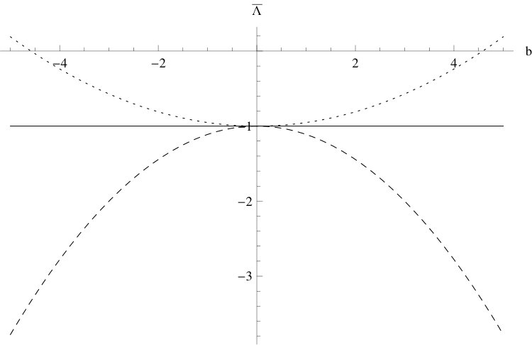 Figure 11
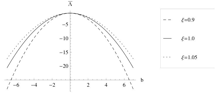 Figure 12
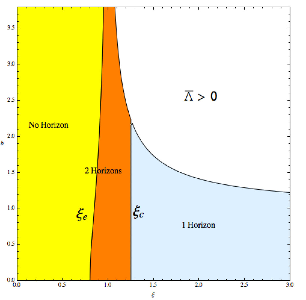 Figure 13
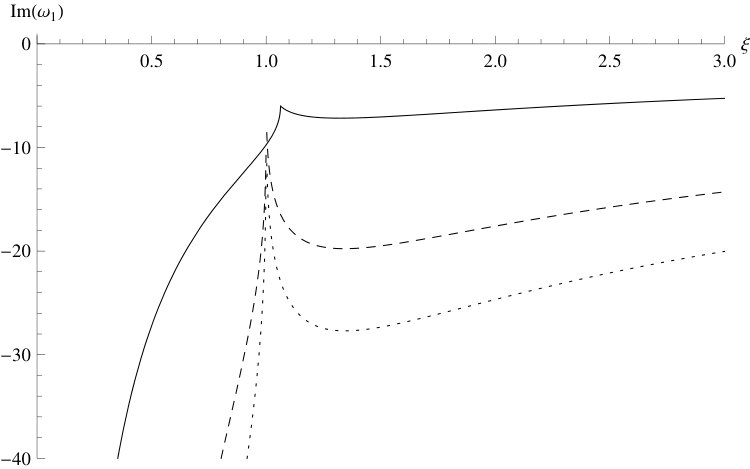 Figure 14
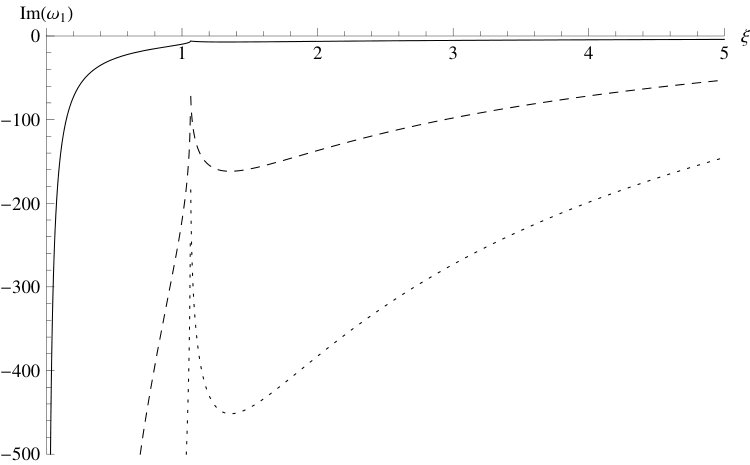 Figure 15
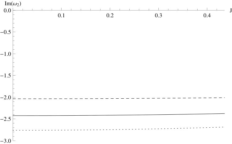 Figure 16
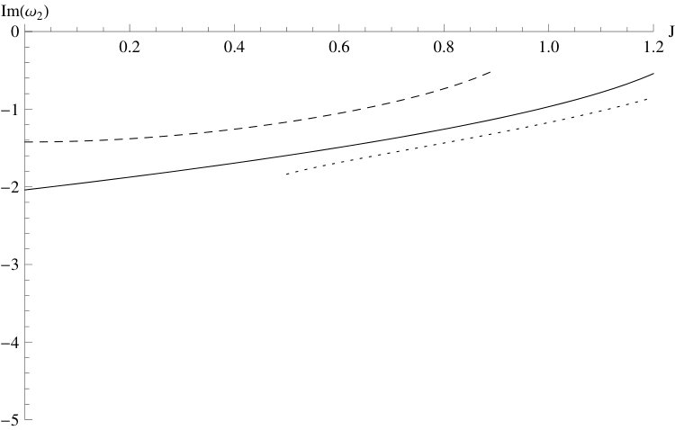 Figure 17
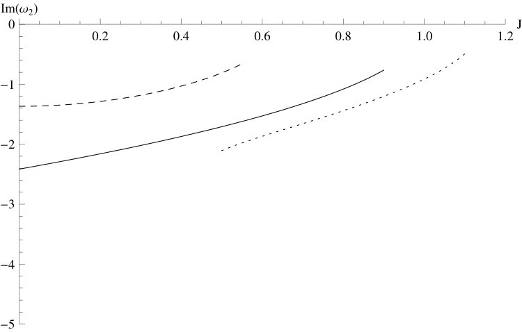 Figure 18
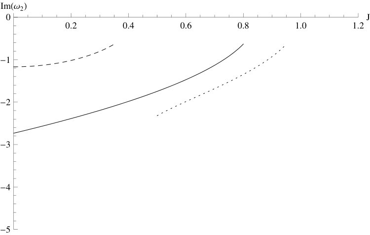 Figure 19
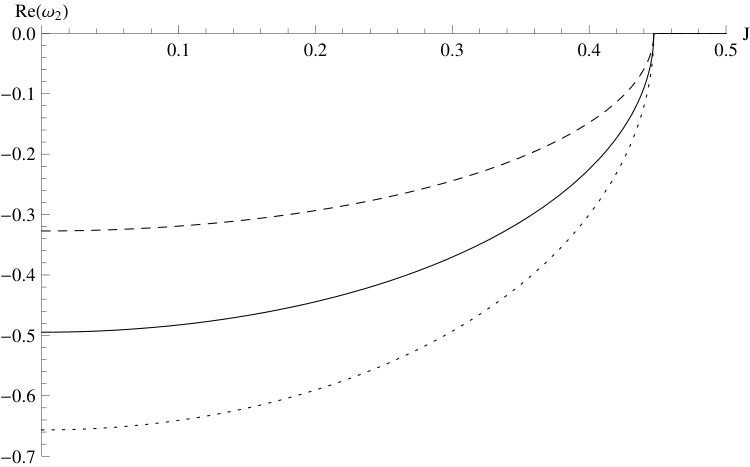 Figure 20
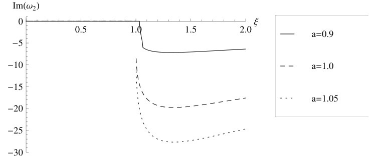 Figure 21
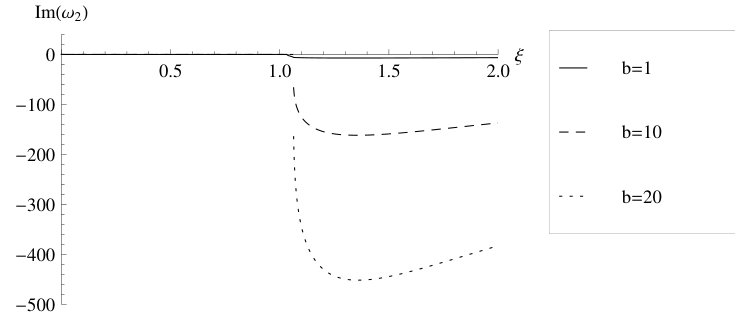 Figure 22
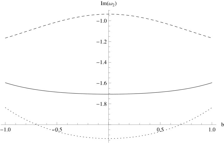 Figure 23
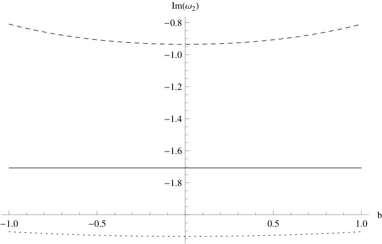 Figure 24
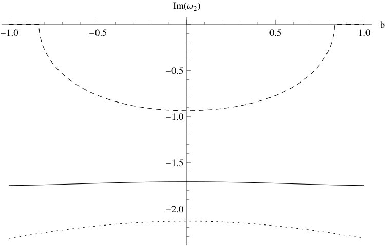 Figure 25
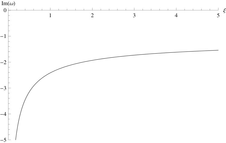 Figure 26
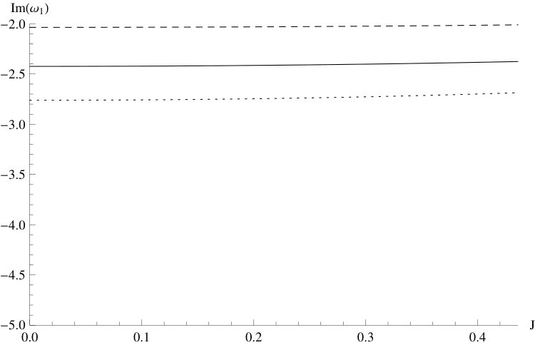 Figure 27
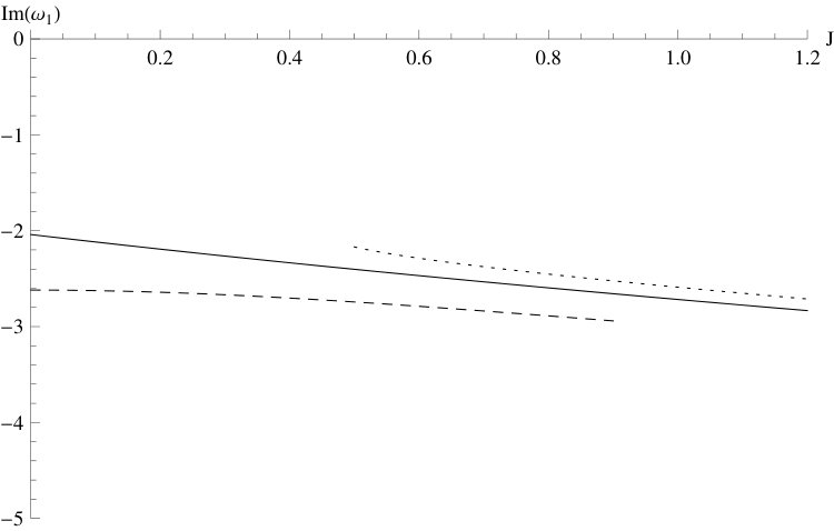 Figure 28
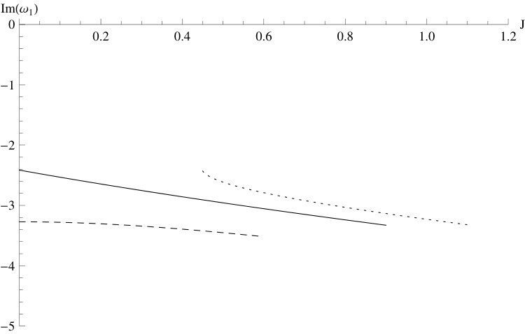 Figure 29
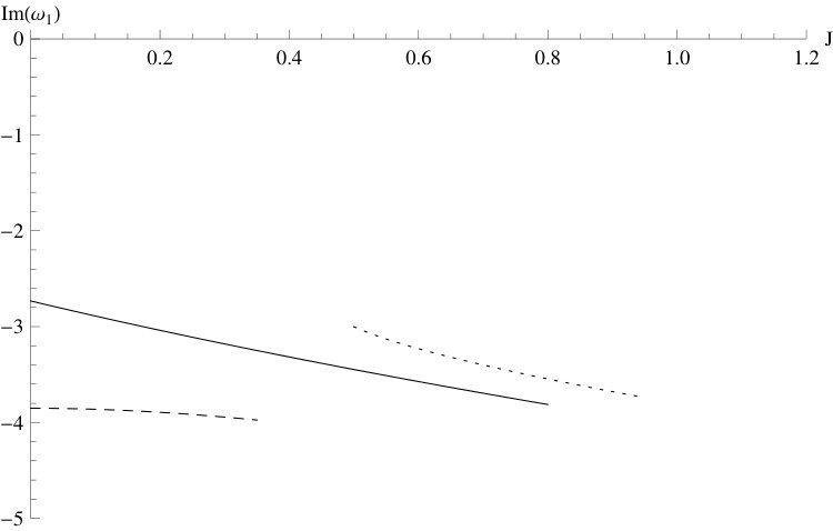 Figure 30
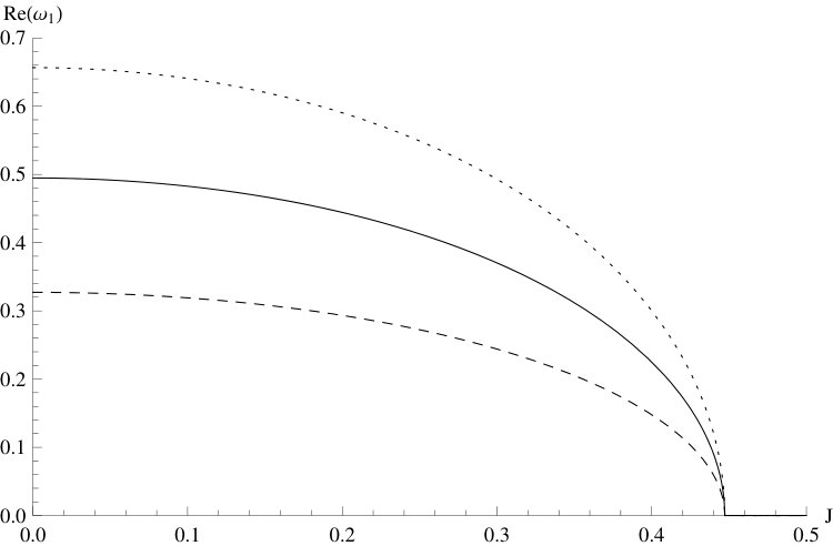 Figure 31
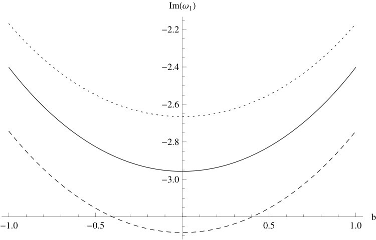 Figure 32
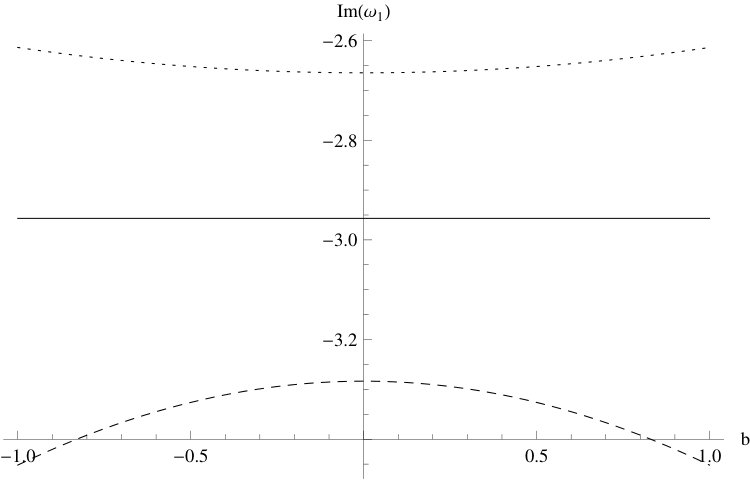 Figure 33
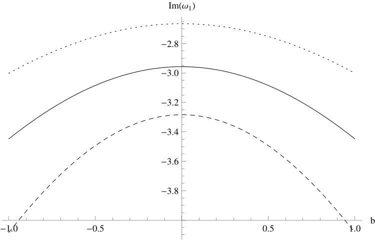 Figure 34
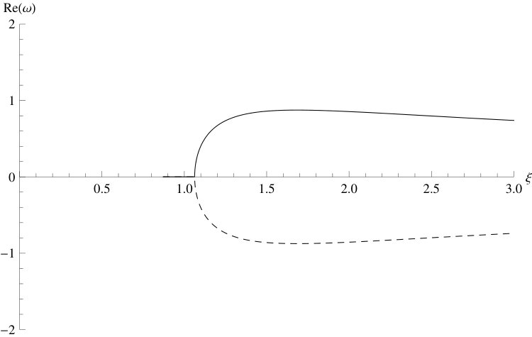 Figure 35
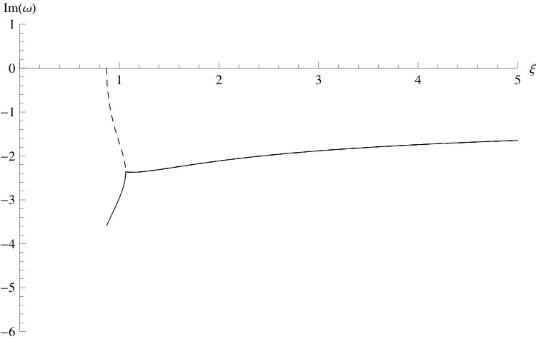 Figure 36
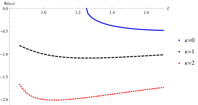 Figure 37
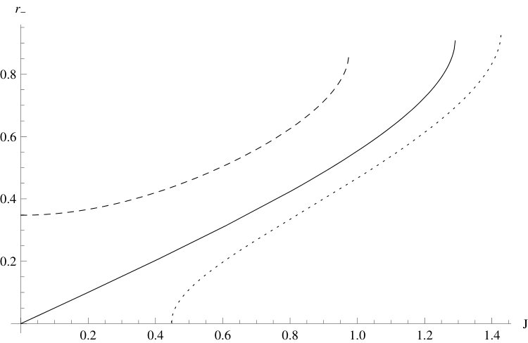 Figure 38
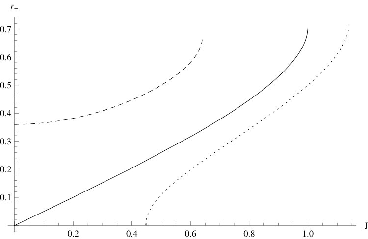 Figure 39
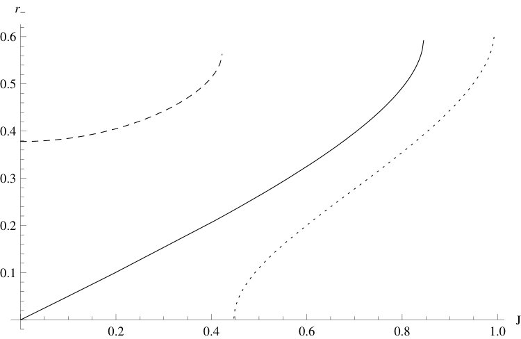 Figure 40
Peer Reviews
No public reviews on file for this paper yet. If you reviewed it on a platform where reviews are public (OpenReview, ICLR, NeurIPS, ICML), you can paste yours below so the community can read it here.
Videos
No videos yet. Explain this paper in a talk, walkthrough, or lecture? Add one.
Quasinormal modes of three-dimensional rotating
Hořava AdS black hole and the approach to thermal equilibrium
Ramón Bécar
Departamento de Ciencias Matemáticas y Físicas, Universidad Católica de Temuco, Montt 56, Casilla 15-D, Temuco, Chile
P. A. González
Facultad de Ingeniería y Ciencias, Universidad Diego Portales, Avenida Ejército Libertador 441, Casilla 298-V, Santiago, Chile.
Eleftherios Papantonopoulos
Department of Physics, National Technical University of Athens, Zografou Campus GR 157 73, Athens, Greece.
Yerko Vásquez
Departamento de Física y Astronomía, Facultad de Ciencias, Universidad de La Serena,
Avenida Cisternas 1200, La Serena, Chile.
Abstract
We compute the quasinormal modes (QNMs) of a massive scalar field in the background of a rotating three-dimensional Hořava AdS black hole, and we analyze the effect of the breaking of the Lorentz invariance on the QNMs. Imposing on the horizon that there are only ingoing waves and at infinity the Dirichlet boundary conditions and the Neumann boundary condition, we calculate the oscillatory and the decay modes of the QNMs. We find that the propagation of the scalar field is stable in this background and employing the holographic principle we find the different times of the perturbed system to reach thermal equilibrium for the various branches of solutions.
I Introduction
If a dynamical system is perturbed, it will return to equilibrium, and this process is completely determined by the poles of the retarded correlation function of the perturbation. In gravity theories, black holes are thermodynamical systems and perturbations of them at equilibrium are described by the quasi-normal modes (QNMs) Regge:1957td ; Zerilli:1971wd ; Zerilli:1970se ; Kokkotas:1999bd ; Nollert:1999ji ; Berti:2009kk ; Konoplya:2011qq . The QNMs are determined by solving the wave equation of an incident wave with the right boundary conditions. Then the solution of the wave equation determines the complex frequencies, the real part of which gives the rate of oscillations of the wave while their complex part gives the required decay time for the system to reach thermal equilibrium.
The QNMs and quasi-normal frequencies (QNFs) have been the subjects of study for a long time and have recently acquired great interest due to the detection of gravitational waves Abbott:2016blz . Despite the detected signal being consistent with the Einstein gravity TheLIGOScientific:2016src , there are great uncertainties in mass and angular momenta of the ringing black hole, which leaves open possibilities for alternative theories of gravity Konoplya:2016pmh like gravity Starobinsky:1980te ; DeFelice:2010aj ; Nojiri:2005jg and Galileon gravity theories Nicolis:2008in ; Deffayet:2009wt ; Kolyvaris:2011fk . Also, the QNMs and the QNFs were extensively studied in connection with the stability of black holes in Einstein gravity Wang:2000gsa ; Wang:2004bv and in modified gravity theories Konoplya:2018qov ; Abdalla:2018ggo ; Abdalla:2019irr .
The gauge/gravity duality which results from the AdS/CFT correspondence Maldacena:1997re ; Aharony:1999ti stimulated the interest in calculating the QNMs and QNFs of black holes in AdS spacetime. It was shown in Birmingham:2001pj that this holographic principle leads to the existence of a correspondence between the QNMs in AdS black holes and linear response theory in scale invariant finite temperature field theory. This correspondence of the decay of perturbations in the dual conformal field theory and the QNMs in the gravity bulk was first discussed in Horowitz:1999jd . Considering the -dimensional AdS black hole BTZ , it was shown analytically Birmingham:2001pj that there is an agreement between its QNFs and the location of the poles of the retarded correlation function describing the linear response on the conformal field theory side.
In this work we will consider a matter distribution in the background of three-dimensional rotating Hořava AdS black holes Sotiriou:2014gna , parameterized by a scalar field. We will perturb the scalar field assuming that there is no back reaction on the metric. This will result in the calculation of the QNMs, which are characterized by a spectrum that is independent of the initial conditions of the perturbation and depends only on the black hole and probe field parameters, and on the fundamental constants of the system (for a review see Siopsis:2008xz ). Exact solutions for QNMs of black holes in three spacetime dimensions have been obtained in exactQNM .
The motivation for considering the Hořava gravity theory is twofold. Considering a condensed matter dynamical system, it was argued in Nicolis:2015sra that this condensed matter system breaks Lorentz invariance spontaneously and its excitations, the superfluid’s phonons, have to non-linearly realize the spontaneously broken Lorentz boosts forcing their interactions to have a very constrained structure. Then, to holographically describe such a system on the boundary, we need to have a Lorentz braking gravity theory in the bulk. The other motivation is, by calculating the QNMs, to see what is the effect of Lorentz breaking symmetry on the relaxation time of the dynamical system to reach thermal equilibrium on the boundary Papantonopoulos:2011zz .
In this context, the QNMs for four-dimensional non-reduced Einstein-aether theory was studied, and it was found in Konoplya:2006rv that the oscillation and damping rate of QNMs are larger than those of Schwarszschild black holes of the Einstein theory, for an effective potential that is known only numerically. More recently, the QNMs for two kinds of aether black holes were analyzed, and it was shown that quasinormal ringing of the first kind of aether black hole is similar to that of another Lorentz violation model-the QED-extension limit of standard model. Also, it was found in Ding:2017gfw that both the first and the second kind of aether black holes have larger damping rate and smaller real oscillation frequency of QNMs compared to Schwarzschild black hole.
The work is organized as follows. In Sec. II after giving a brief review of the BTZ black hole, we discuss the three-dimensional Hořava gravity and its connection with three-dimensional Einstein-aether theory. In Sec. III we find the QNMs analytically for massive scalar fields with circular symmetry and for a specify value of . Also, for massive scalar field we show that the Klein-Gordon equation can be written as the Heun’s equation, and we find the QNFs numerically by applying the pseudospectral method. Finally, our conclusions are in Sec. IV.
II Three-dimensional Rotating Hořava Black Holes
In this Section, after reviewing in brief the BTZ black hole, we discuss the Hořava gravity and its connection with three-dimensional Einstein-aether theory. The metric of the BTZ black hole is given by
[TABLE]
The angular coordinate has period , and the radii of the inner and outer horizons are denoted by and , respectively. The dual conformal field theory on the boundary is -dimensional, the conformal symmetry being generated by two copies of the Virasoro algebra acting separately on left- and right-moving sectors Birmingham:2001pj . Consequently, the conformal field theory splits into two independent sectors at thermal equilibrium with temperatures
[TABLE]
According to the AdS3/CFT2 correspondence, to each field of spin propagating in AdS3 there corresponds an operator in the dual conformal field theory characterised by conformal weights with Aharony:1999ti
[TABLE]
and is determined in terms of the mass of the scalar field,
[TABLE]
For a small perturbation, one expects that at late times the perturbed system will approach equilibrium exponentially with a characteristic time-scale. This time-scale is inversely proportional to the imaginary part of the poles, in momentum space, of the correlation function of the perturbation operator . For a conformal field theory at zero temperature, the 2-point correlation functions can be determined, up to a normalisation, from conformal invariance.
Then two sets of poles were found Birmingham:2001pj
[TABLE]
where takes the integer values . This set of poles characterises the decay of the perturbation on the CFT side, and coincides precisely with the quasi-normal frequencies of the BTZ black hole Birmingham:2001pj .
We now discuss the three-dimensional Hořava gravity, the action of which is given by Sotiriou:2011dr
[TABLE]
where is a coupling constant with dimensions of a length squared and the Lagrangian has the following form
[TABLE]
where , , and correspond to extrinsic, mean, and scalar curvature, respectively, and is a parameter related to the lapse function via , being the line element in the preferred foliation
[TABLE]
Also, is the determinant of the induced metric on the constant- hypersurfaces. corresponds to a set of all the terms with four spatial derivatives that are invariant under diffeomorphisms. For and , the action reduces to that of General Relativity. In the infrared limit of the theory the higher order terms (UV regime) can be neglected, and the theory is equivalent to a restricted version of Einstein-aether theory, through
[TABLE]
and
[TABLE]
where . Being the action of Einstein-aether:
[TABLE]
where is a coupling constant with dimensions of a length square, is the determinant of , is the cosmological constant, is the Ricci scalar,
[TABLE]
and
[TABLE]
Another important characteristic of this theory is that only in the sector , Horava gravity admits Asymptotically AdS solution Sotiriou:2014gna . Therefore, assuming stationary and circular symmetry, the theory will admit the BTZ analogue to the three-dimensional rotating Hořava black holes described by metric
[TABLE]
where
[TABLE]
with
[TABLE]
where and are constants that can be regarded as measures of aether misalignment, with as a measure of asymptotically misalignment, for , the aether does not align with the timelike Killing vector asymptotically. Note that when and , the solution becomes BTZ black holes, and for , the solution becomes BTZ black holes with a shifted cosmological constant, . Also, can be negative, when either or , . The sign of determine the asymptotic behavior (flat, dS, or AdS) of the metric Sotiriou:2014gna .
In Sotiriou:2014gna was argued that if , and the aether represents a well defined folation at large for any value of . Moreover, if , then is always negative for any . Also, if the coupling constants are such that , and , then ÃÑ will switch sign at some value of b.
In Fig. 1 we show the behavior of as a function of . When increases (left panel), we observe a region where there is no a horizon until for which the black hole becomes extremal, this value can be obtained from . Then there is a region where increases and decreases until becomes null when , and finally there is a region where there is only one horizon. Also, we can observe the same behavior when decreases (right panel). Also, in Figs. 2 and 3, we plot the behavior of as a function of , and its sign determines the asymptotic behavior (flat, dS, or AdS) of the metric. Note that for , the sign of is negative, as mentioned, if the coupling constants are such that , and , then will switch sign at some value of b.
The value of for which the black hole is extremal is given by
[TABLE]
the value of for which the black hole passes from having two horizons to having one horizon, an is given by
[TABLE]
and the value of for which the effective cosmological constant changes sign is given by . In Fig. (4) we plot the different regions defined by , , and for a choice of parameters.
In the case (), there is a curvature singularity due to the Ricci scalar
[TABLE]
is divergent at . This is in contrast to BTZ black holes where the Ricci and Kretschmann scalars are finite and smooth at . The locations of the inner and outer horizons , are given by
[TABLE]
Also, and can be written as and , respectively. The Hawking temperature is given by
[TABLE]
III QNMs
The quasi-normal modes of scalar perturbations for a minimally coupled massive scalar field to curvature on the background of three-dimensional Hořava AdS black holes are described by the solution of the Klein-Gordon equation
[TABLE]
where is the mass of the scalar field . Which can be written as
[TABLE]
The term is given by
[TABLE]
It is worth mentioning that the second term in the above expression vanishes for . Performing the change of variables along with the ansatz , Eq. (23) yields
[TABLE]
III.1 Massive scalar field with circular symmetry
For a massive scalar field with circular symmetry () Eq. (III) is
[TABLE]
which can be written as
[TABLE]
where
[TABLE]
Under the decomposition , Eq. (27) can be written as a hypergeometric equation for
[TABLE]
where the coefficients , , and are given by
[TABLE]
and the exponents and are
[TABLE]
The general solution of Eq. (29) takes the form
[TABLE]
which has three regular singular points at , , and . Here, is a hypergeometric function and , are constants. Then, without loss of generality, we choose the negative sign for , and the solution for the radial function is
[TABLE]
According to our change of variables at the vicinity of the horizon , , and at infinity , . In the vicinity of the horizon, and using the property , the function behaves as
[TABLE]
and the scalar field can be written in the following way
[TABLE]
in which the first term represents an ingoing wave and the second term an outgoing wave in the black hole. To compute the QNMs, we have to impose the boundary conditions on the horizon that there exist only ingoing waves. This fixes . So, the radial solution becomes
[TABLE]
In order to implement boundary conditions at infinity (), we shall apply in Eq. (36), the Kummer’s formula, for the hypergeometric function M. Abramowitz ,
[TABLE]
With this expression, the radial function results in
[TABLE]
Therefore, by imposing that the scalar field at infinity is null, for ( and ), then the term proportional to in Eq. (III.1) diverges. So, we obtain that the scalar field is null only upon the following additional restriction or . Then, the QNFs yields
[TABLE]
[TABLE]
respectively. Note that the imaginary part of the QNFs is negative, which ensures that the propagation of scalar fields is stable in this background.
Now, in order to observe the behavior of the QNFs (39) and (40), we plot in Fig. 5, the behavior of the real (left panel) and imaginary parts (right panel) of the fundamental QNFs as a function of . Note that, as mentioned, for , there is no horizon. So, for , we observe that for (continuous line) there is a range where is null and then takes positive values, when the coupling constant increases, while decreases when increases. So, according to the gauge/gravity duality, the relaxation time in order to reach the thermal equilibrium increases for the right sector. However, for (dashed line) and , is null and then takes negative values, while its imaginary part increases and then decreases when the coupling constant increases, showing that the relaxation time can decrease or increase depending on the value of . It is interesting to note that when decreases . If we consider the BTZ black hole, and , the real part is null and . In the following, we will analyze the two branches of QNFs for different values of . Fig. (6) is similar to Fig. (5), but in order to see the effect of on the behavior of the QNFs, we have plotted several curves corresponding to different values of parameter . For the QNFs coincide and correspond to the QNFs of the BTZ black hole. On the other hand, for , both purely imaginary branches converge to the same value. For values of near 1, decreases when increases, decreasing faster for large values of , while increases when increases, increasing faster for small values of , which implies that the relaxation time of the right sector increases and the relaxation time of the left sector decreases. On the other hand, we observe that for near with , only one branch exists, and decreases for small values of while it increases for large values of . Notice that for the effective cosmological constant becomes positive before reaching the value .
III.1.1
Now, in order to observe the behavior of the QNFs (39) and (40), in the range , that is, where are positive, first we plot versus in Fig. 7, for different values of the parameters and , in order to see for which values of the parameter the horizons are positive. Then, for this range, we plot the imaginary part of the QNFs in Fig. 8, and we observe that for , increases when the parameter (or equivalently , see Fig. 9) increases, see left panel of Fig. 8, so the relaxation time decreases. However, for , the behavior is the opposite. decreases when the parameter increases, see right panel of Fig. 8, so the relaxation time increases. Note that in this range is null. Also, the sectors and of the conformal field theory are well defined. Furthermore, decreases and increases, when the coupling constant increases; so, the relaxation time increases and decreases, respectively.
In Fig. 10 we plot the fundamental QNFs as a function of . We observe that for the BTZ black hole, the central panel with , the imaginary part of the fundamental QNF is constant; however, for a asymptotical misalignment of the aether with the timelike Killing vector, , the fundamental QNFs depend on . increases when decreases. For the behavior is the opposite since it decreases when decreases.
III.1.2
As mentioned, for there is only one horizon. and become imaginary. This occurs for , and consequently there is a gap in , see Fig. 7, left panel, and for which is negative, see Fig. 9, which occurs when . In Fig. 11, we plot the fundamental QNFs for the range of values of in which it is positive, and there is only one horizon. So, we observe that the fundamental QNFs acquire a real part, with , decreases when increases, and , and it is negative. In this case, the two branches have converge to one branch and when the coupling constant increases decreases, see Fig. 5.
III.1.3
Finally, for , that is , the two sectors converge, this occurs for , that is . In this case the QNFs are given by
[TABLE]
where . In Fig. 12 we show the behavior of the fundamental QNFs as a function of . We observe that decreases when increases whereas is null. So, according to the gauge/gravity duality, the relaxation time in order to reach the thermal equilibrium increases.
Finally, we plot in Fig. 13 for different values of the constants and . We observe that for the range , increases when the constants or increase, so the relaxation time decreases.
Neumann boundary conditions. The frequencies found above for the scalar perturbation have been obtained by imposing the vanishing Dirichlet boundary condition at infinity. It is known that the Dirichlet boundary condition does not lead to any quasinormal modes for . However, it is also possible to find a second set of QNFs, for negative mass squared, if we consider that the flux of the scalar field vanishes at infinity or vanishing Neumann boundary condition at infinity, which allows us to describe tachyons. Furthermore, it was shown that for negative mass squared there are two sets of dual operators and , where the second set of QNFs matches exactly the dual operators with Birmingham:2001pj . So, by using the condition that the flux, which is given by
[TABLE]
vanishes at asymptotic infinity, we obtain for and , that the flux vanishes if or , which leads to
[TABLE]
[TABLE]
respectively.
III.2 Massive scalar field
For massive scalar field, the Klein-Gordon equation can be rewritten as
[TABLE]
where
[TABLE]
and
[TABLE]
Under the decomposition , with
[TABLE]
Eq.(45) can be written as
[TABLE]
where
[TABLE]
[TABLE]
that corresponds to Heun’s differential equation. The condition , ensures regularity of the point at , and corresponds to the accessory parameter. Heun’s equation has four regular singular points: , and with exponents , , , and . Now, in order to obtain the QNFs, we proceed to perform a numerical analysis by using the pseudospectral Chebyshev method Boyd , which has been applied to compute the QNFs in other geometries, for instance see Gonzalez:2017shu ; Gonzalez:2018xrq ; Finazzo:2016psx . In Fig. 14 we plot the numerical results obtained for the real and imaginary parts of the fundamental QNF of the branch as a function of for different values of . We observe that for , the absolute value of the imaginary part decreases as increases; however, for , the behavior is the opposite; the absolute value of the imaginary part increases as increases. Note that, for the cases analyzed, the QNFs have a negative imaginary part, which ensures that the propagation of scalar fields is stable in this background.
III.3 Case: or
In this case, Eq. (45) becomes
[TABLE]
where , , and are given by Eq. (46). Under the decomposition , Eq. (52) can be written as a hypergeometric equation for , Eq. (29), where the coefficients , and are given by
[TABLE]
and the exponents and are
[TABLE]
Following the same procedure detailed in the case of massive radial scalar field we obtain for ( and ) that the field at infinity is null if the gamma function has the poles at for . Then, the wave function satisfies the considered boundary condition only upon the following additional restriction or . These conditions determine the form of the QNFs as
[TABLE]
[TABLE]
respectively.
Now, in a similar manner to the first case, that is, using the condition that the flux vanishes at asymptotic infinity, we obtain for and , with or , the second set of QNFs, which yields
[TABLE]
[TABLE]
respectively. In this case, the QNFs correspond to , where are the QNFs for massive radial scalar fields. So, the condition ( or ) only has effect on the real part of the QNFs. As mentioned, when (=), the solution results in the BTZ black holes with a shifted cosmological constant, . Note that the QNFs have real and imaginary parts, with an imaginary part that is negative, which ensures that the propagation of scalar fields is stable in this background.
IV Remarks and conclusions
In this work, we computed the QNMs of rotating three-dimensional Hořava AdS black holes and we analyzed the effect of the breaking of the Lorentz invariance on the QNMs. We showed that depending on the parameters, the lapsus function can represent a spacetime without an event horizon, a black hole geometry with one event horizon, an extremal black hole and finally a black hole with two horizons. The QNMs have been obtained by imposing on the horizon that there are only ingoing waves, while at infinity Dirichlet boundary conditions and Neumann boundary conditions were imposed. We found that the propagation of the scalar field is stable in this background, since the imaginary part of the QNFs is negative. Also, we made a systematic study of the QNMs and QNFs for various ranges of parameters , the angular momentum and the parameter that differentiates Horava gravity from General Relativity which is obtained for . For various values of and , we obtained various branches of solutions with different properties of QNMs and QNFs. In particular:
For positive inner and outer horizons , the range gives null for the fundamental QNFs, and the two sectors and are well defined. increases when the parameter increases, so according to the gauge/gravity duality, the relaxation time in order to reach the thermal equilibrium decreases. Furthermore, as the coupling constant increases, decreases and therefore the relaxation time increases. However, for , the behavior is opposite. decreases when the parameter increases and therefore the relaxation time increases. Furthermore, increases when increases; so, the relaxation time decreases.
In the range the black hole only has one horizon . For this case and the QNFs acquire a real part, with , decreases when increases, and , and it is negative. Also, when increases, decreases. Finally, for , that is, , the two sectors converge. This occurs when . In this case decreases when increases whereas is null. Therefore, the relaxation time increases. Also, we have considered different values of the constants and , and increases when the constant or increases; so, the relaxation time decreases.
Moreover, for the general case, that is, a massive scalar field, it was shown that the Klein-Gordon equation can be written as the Heun’s differential equation, and we have studied the behavior of the QNMs numerically via the pseudospectral Chebyshev method, and mainly it was found that for and , the absolute value of the imaginary part decreases as increases; however, for the behavior is the opposite. The absolute value of the imaginary part increases as increases.
As can be seen from the above discussion, the oscillatory and the decay modes of the QNMs have quite different behavior for the various branches, indicating that the time required for a system to reach thermal equilibrium on the boundary is different for the various values of the parameters. An intriguing result is that if the parameter lies between two different critical values, then the time required for the two sectors and to reach thermal equilibrium is competing in the sense that in one sector the time is increasing while in the other sector it is decreasing. This behavior deserves further study in connection of trying to find a system on the boundary that exhibits such a behavior.
It would be interesting to extent this work to higher dimensional Horava black holes Koutsoumbas:2010pt and calculating the QNMs and QNFs of a massive wave to study how a gravity theory in the bulk with broken Lorentz invariance affects the boundary field theory to reach thermal equilibrium.
Acknowledgments
This work was funded by the Dirección de Investigación y Desarrollo de la Universidad de La Serena (Y.V.). E.P., Y.V. and R.B would like to thank the Facultad de Ingeniería y Ciencias, Universidad Diego Portales for its hospitality, where part of this work was carried out.
The reference list from the paper itself. Each links out to its DOI / PubMed record.
- 1(1) T. Regge and J. A. Wheeler, “Stability Of A Schwarzschild Singularity,” Phys. Rev. 108 , 1063 (1957).
- 2(2) F. J. Zerilli, “Gravitational field of a particle falling in a schwarzschild geometry analyzed in tensor harmonics,” Phys. Rev. D 2 , 2141 (1970).
- 3(3) F. J. Zerilli, “Effective Potential For Even Parity Regge-Wheeler Gravitational Perturbation Equations,” Phys. Rev. Lett. 24 , 737 (1970).
- 4(4) K. D. Kokkotas and B. G. Schmidt, “Quasi-normal modes of stars and black holes,” Living Rev. Rel. 2 , 2 (1999) [ar Xiv:gr-qc/9909058].
- 5(5) H. P. Nollert, “TOPICAL REVIEW: Quasinormal modes: the characteristic ‘sound’ of black holes and neutron stars,” Class. Quant. Grav. 16 , R 159 (1999).
- 6(6) E. Berti, V. Cardoso and A. O. Starinets, “Quasinormal modes of black holes and black branes,” Class. Quant. Grav. 26 , 163001 (2009) [ar Xiv:0905.2975 [gr-qc]].
- 7(7) R. A. Konoplya and A. Zhidenko, “Quasinormal modes of black holes: from astrophysics to string theory,” Rev. Mod. Phys. 83 , 793 (2011) [ar Xiv:1102.4014 [gr-qc]].
- 8(8) B. P. Abbott et al. [LIGO Scientific and Virgo Collaborations], “Observation of Gravitational Waves from a Binary Black Hole Merger,” Phys. Rev. Lett. 116 , no. 6, 061102 (2016) [ar Xiv:1602.03837 [gr-qc]].