Some results for the large time behavior of Hamilton-Jacobi Equations with Caputo Time Derivative
Olivier Ley, Erwin Topp, Miguel Yangari

TL;DR
This paper investigates the large time behavior of solutions to Hamilton-Jacobi equations with Caputo fractional time derivatives, establishing regularity estimates and partial convergence results under certain geometric conditions.
Contribution
It provides the first regularity estimates and convergence insights for Hamilton-Jacobi equations with fractional Caputo derivatives, extending classical results to fractional time derivatives.
Findings
Hölder regularity estimates independent of time
Counterexample showing non-convergence with nonpositive Caputo derivative
Partial convergence results under geometric assumptions
Abstract
We obtain some H\"older regularity estimates for an Hamilton-Jacobi with fractional time derivative of order cast by a Caputo derivative. The H\"older seminorms are independent of time, which allows to investigate the large time behavior of the solutions. We focus on the Namah-Roquejoffre setting whose typical example is the Eikonal equation. Contrary to the classical time derivative case , the convergence of the solution on the so-called projected Aubry set, which is an important step to catch the large time behavior, is not straightforward. Indeed, a function with nonpositive Caputo derivative for all time does not necessarily converge; we provide such a counterexample. However, we establish partial results of convergence under some geometrical assumptions.
Click any figure to enlarge with its caption.
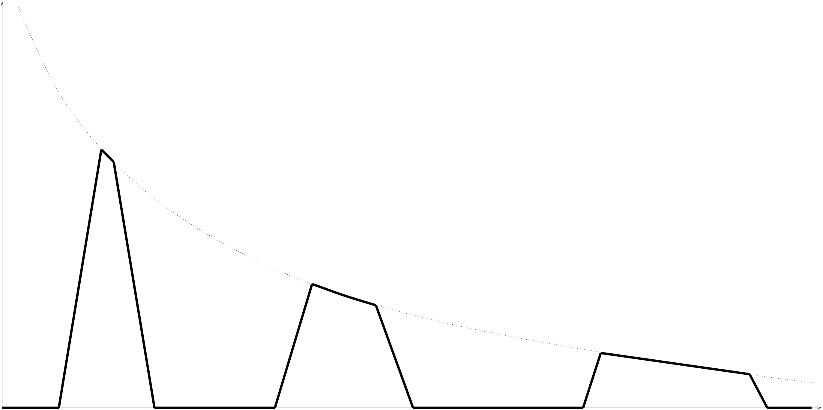 Figure 1
Peer Reviews
No public reviews on file for this paper yet. If you reviewed it on a platform where reviews are public (OpenReview, ICLR, NeurIPS, ICML), you can paste yours below so the community can read it here.
Videos
No videos yet. Explain this paper in a talk, walkthrough, or lecture? Add one.
Some results for the large time behavior of Hamilton-Jacobi Equations with Caputo Time Derivative
Olivier Ley
Olivier Ley: Univ Rennes, INSA Rennes, CNRS, IRMAR - UMR 6625, F-35000 Rennes, France.
,
Erwin Topp
Erwin Topp: Departamento de Matemática y C.C., Universidad de Santiago de Chile, Casilla 307, Santiago, CHILE.
and
Miguel Yangari
Miguel Yangari: Departamento de Matemática, Escuela Politécnica Nacional, Ladrón de Guevara E11-253, P.O. Box 17-01-2759, Quito, Ecuador.
Abstract.
We obtain some Hölder regularity estimates for an Hamilton-Jacobi with fractional time derivative of order cast by a Caputo derivative. The Hölder seminorms are independent of time, which allows to investigate the large time behavior of the solutions. We focus on the Namah-Roquejoffre setting whose typical example is the Eikonal equation. Contrary to the classical time derivative case , the convergence of the solution on the so-called projected Aubry set, which is an important step to catch the large time behavior, is not straightforward. Indeed, a function with nonpositive Caputo derivative for all time does not necessarily converge; we provide such a counterexample. However, we establish partial results of convergence under some geometrical assumptions.
1. Introduction.
In this note we are interested in nonlocal Hamilton-Jacobi equations with the form
[TABLE]
subject to the initial condition
[TABLE]
for some and given.
The nonlocal nature of the problem is cast by the operator , which denotes the Caputo time derivative of order , starting at time zero. For it is defined as
[TABLE]
where is the Gamma function that acts as a normalizing constant making become the usual first order derivative when , see [10, 16] and references therein. Following the ideas of [3], where under appropriate assumption on the function , its Caputo derivative in (1.3) can be equivalently computed as
[TABLE]
for some , and where we have extended as for . This operator has a nonlocal degenerate elliptic nature in the sense of Barles and Imbert [6] that allows to conclude comparison principle among viscosity solutions as it is proved in [23]. This is a powerful reason to consider Caputo derivative instead of other fractional derivatives, as, for example, Riemann-Liouville derivative defined for adequate functions as
[TABLE]
Moreover, as it can be seen in [10, Chapters 5,6], Caputo derivative is more adequate to deal with the most classical notion of initial condition compared with Riemann-Liouville problems, where the initial condition is understood in a generalized sense.
Coming back to (1.1), and more specifically to the Hamiltonian , we assume throughout this paper is periodic in and coercive in .
We focus our attention into Bellman-type Hamiltonians with the classical structure related to optimal control problems with compact control set, that is, satisfying the regularity/growth condition
[TABLE]
for some , and for all .
We are also interested in the case has superlinear growth in the gradient, common in control problems with unrestricted control space. We refer to this case through the following assumption: there exists (the “gradient growth”) and , such that
[TABLE]
for some and all , . We notice at once that the first condition in (1.6) implies that there exist such that
[TABLE]
and the same inequality holds with if the second condition holds in (1.6) and is convex.
Our interest is the analysis of the behavior of the solutions to (1.1)-(1.2) and make a contrast with the classical case , namely, the Hamilton-Jacobi equation
[TABLE]
There is a vast literature regarding problem (1.8)-(1.2). We refer the surveys of Barles and Ishii in [2] and references therein for the basics about this problem, like existence, uniqueness and regularity.
A natural question that arises is the analysis of the behavior of the solution for long times. There too, there are a lot of references when , see [12, 20, 4, 13, 9, 17, 7, 2] and the references therein. Here, we focus on the nowadays classical framework of Namah and Roquejoffre paper [20], where the authors address the long time behavior of (1.8) under the assumption that
[TABLE]
It is possible to generalize slightly the above assumptions but we choose to state them in this form since all the main difficulties are present.
Under these assumptions, (1.1) reads
[TABLE]
and
[TABLE]
the so-called projected Aubry set [13], which is a compact subset of . It follows from Lions, Papanicolaou and Varadhan [19] that the so-called ergodic problem
[TABLE]
has a solution and is unique. Actually, under our assumptions, it is easy to see that .
It is then expected that the long time behavior of the solution of (1.1)-(1.2) is given by the asymptotic expansion
[TABLE]
where is a solution of (1.12).
In the local case , this asymptotic behavior is established in [20, Theorem 1]. The proof relies basically on three steps. The first step is to obtain that the set is relatively compact in . Let us point out that this property is not sufficient and the main difficulty is to prove the full convergence of as . The second step is to notice that for , from which one infers that is nonincreasing in time on , so it converges uniformly to a Lipschitz continuous function on as . The third step is to take the half-relaxed limits
[TABLE]
which are, respectively, a sub- and a supersolution of (1.12) and then to apply a strong comparison result for (1.12) with the “Dirichlet boundary condition” on . It follows in , which gives the desired full convergence.
Our goal is to develop a similar procedure for the Caputo fractional case . The first step holds. Indeed, the elliptic properties shown by the expression (1.4) are not only related to comparison principles but also to regularity in the time variable. Using Ishii-Lions method for nonlocal problems presented in [5], we are able to prove that bounded solutions to (1.1) are -Hölder continuous in time, uniformly in , see Theorem 2.1. We recall that such a property does not come from the contraction principle given by comparison arguments as in the classical case, basically because such a property is not known for fractional problems, where the influence of the ”memory” put troubles in the analysis of problems shifted in time. Moreover, in the local case (1.8), Lipschitz estimates in time allows to use Rademacher’s Theorem to regard as an function, and extract the boundedness of through the coercivity of . Such a program cannot be carried out directly in (1.1) since -Hölder functions are not sufficient to make in . Nevertheless, we can get equicontinuity in the space variable by a regularization procedure via inf and sup convolutions, see Theorem 2.2.
Similarly, the third step is identical to the one in the classical case since the ergodic problem (1.12) is the same for all .
It follows that the limiting step is the second one. We still have for but it is not anymore sufficient to infer neither that is nonincreasing in time on , nor that it converges. As we show in Section 3, it is possible to have bounded functions with signed -order Caputo derivative, but not converging as , which is a surprising result interesting by itself.
To overcome this difficulty and obtain the convergence on , we need to give additional assumptions on the geometry of and . Precise assumptions are stated in Section 4 but basically, we assume
[TABLE]
These assumptions are inspired from the classical case, where it is known that the solution of (1.8) is the value function of an optimal control problem for which assumptions (1.14)-(1.15) means roughly that we can travel with minimal cost on . But let us point out that these geometrical assumptions are not required in the classical case and that there is no rigorous link between the fractional case and the expected control problem, which could make these ideas rigorous. See Camilli, De Maio, Iacomini [8] for the precise statement of a related control problem which should be associated with the case , and some discussion in this direction.
It follows that we need to translate these ideas in the PDE framework building some suitable supersolutions, which tends to 0 thanks to (1.14)-(1.15). By comparison, we obtain estimates
[TABLE]
where is a rectifiable curve on joining and , and is the solution of a fractional ODE with limit 0 at ; see Theorem 4.3 and Theorem 4.5 for an extension to some possibly infinite length curves. This implies the convergence of on from which we deduce easily (1.13), see Corollary 4.7. This approach is new but we think it does not provide optimal results. In particular, it relies too heavily on the geometry of , which is not the case in the classical approach described above for . To go further, one would need some quantitative estimates on how much nonpositive is , which seems difficult to obtain, even in the case .
The paper is organized as follows. We start by introducing precisely the Caputo fractional operator and recalling some useful properties. Then we establish some regularity estimates for the solution of (1.1) in Section 2. Section 3 is devoted to a counterexample showing that a bounded function with nonnegative Caputo derivative does not necessarily converges. Finally, some positive results for the large time behavior of the solution of (1.1) are proved in Section 4.
Notations and preliminaries. We will write the Caputo derivative using (1.4) (with for simplicity). More precisely, let . We extend to by setting for and define, when it exists, for every and ,
[TABLE]
where, for , we set
[TABLE]
Notice that is well-defined as soon as and is in a neighborhood of . More about the functional formulation of this operator can be found in the references [18, 10, 16]. For the definition of viscosity solutions to (1.1), we refer to [6, 23].
Notice that for all , there exists such that
[TABLE]
We introduce the Mittag-Leffler functions of order as in [10, Definition 4.1]. Recall that is smooth on , and we have the following useful properties
[TABLE]
We will write for every .
2. Regularity Estimates
We start with a regularity result in time for bounded solutions to (1.1). This result is a consequence of the Hölder estimates reported by Barles, Chasseigne and Imbert in [5].
Theorem 2.1**.**
Assume (1.5) or (1.6), and . Let be bounded, continuous viscosity solution to (1.1)-(1.2). Then, is Hölder continuous in time, that is there exists a constant large enough such that
[TABLE]
The constant depends on the data and but does not depend on .
Proof.
Despite the proof we present here is valid for both (1.5) and (1.6), we underline the arguments in the later case. Let be away from zero, and denote . If (1.6) is assumed, then we consider , and if (1.5) is assumed, then in what follows.
Using the linearity of the Caputo derivative, it is direct to check that solves
[TABLE]
with initial condition .
By (1.17) and , we have that are respectively super- and subsolutions of (1.1)-(1.2) for large enough depending only on and . Therefore, a direct application of the comparison results in [23] leads to the estimates
[TABLE]
These bounds can be readily adapted to by multiplying by the last inequality.
By contradiction, assume that for all we have
[TABLE]
Taking very close to in term of above, we can get
[TABLE]
For localization purposes, we introduce a function with the following properties: we consider smooth and nondecreasing, such that if , if , and for small we denote . Then, for all small enough, we have
[TABLE]
where we recall that we extend as for negative times .
Then, for small we define
[TABLE]
We have that attains its maximum at a point and this maximum is bigger than .
Standard arguments lead to
[TABLE]
where as if is fixed ( is a modulus of continuity in space of in the compact set ), and
[TABLE]
for some constant just depending on . In particular, for large enough we may assume that .
Below, we use a constant , which may vary line to line but only depend on the data of the problem and not on nor .
Here we claim that for all large, and small in terms of . In fact, if (the case is analogous), then, using (2.3), we see that
[TABLE]
where is the Lipschitz constant of . Taking , we arrive at
[TABLE]
which is a contradiction if is taken small, and close to in terms of .
In addition, since is uniformly continuous in space, then for all large enough and small in terms of . Indeed, if , then we would have
[TABLE]
Hence, for and fixed, taking small and close to , we arrive at a contradiction.
Since and , we can use the penalization defining as a testing for . For this, in what follows we write , from which we see that
[TABLE]
At this point, denoting we notice that the function
[TABLE]
has a local maximum point at , from which we can use the subsolution’s viscosity inequality to write, for all , that
[TABLE]
Similarly, denoting we notice the function
[TABLE]
has a local minimum point at , from which we can use the supersolution’s viscosity inequality to write, for all , that
[TABLE]
Then, we subtract both inequalities to arrive at
[TABLE]
where, noticing that , we write
[TABLE]
From (1.6), we get
[TABLE]
and from here, taking , we conclude that
[TABLE]
where just depends on .
Consider and we split the term as
[TABLE]
with
[TABLE]
We start with . Directly from the definitions, we see that
[TABLE]
where as independent of the rest of the variables by the smoothness of . Now, performing the change of variables in the first integral, and in the second, we arrive at
[TABLE]
where the last equality comes from the symmetry of the kernel. Performing a second order expansion and recalling that , we obtain that there exists such that
[TABLE]
Therefore,
[TABLE]
and from here
[TABLE]
Now we deal with , writing
[TABLE]
where depends only on .
To deal with the remaining term , we assume that (the case follows the same lines). Performing similar change of variables as above and using the maximal inequality we arrive at
[TABLE]
Noticing that the smooth function satisfies , we conclude that . From this
[TABLE]
Joining this with (2.7) and (2.8) in (2.6) we get
[TABLE]
Then, we let first, then and finally and, having taken large enough just in terms of the data and , we reach a contradiction. It ends the proof. ∎
Now we would like to obtain estimates in space.
Theorem 2.2**.**
Assume hypotheses of Theorem 2.1 hold. For each bounded viscosity solution to (1.1), there exists a modulus of continuity independent of such that
[TABLE]
If, in addition, satisfies (1.7) for some , then, for each , there exists a constant such that
[TABLE]
The modulus and the constant depend on the datas and but do not depend on .
Proof.
For , we introduce the sup-convolution
[TABLE]
We collect some properties of this regularization of :
- (i)
is still Hölder continuous in time satisfying (2.1) like ,
- (ii)
,
- (iii)
is Lipschitz continuous in time with Lipschitz constant with just depending on ,
- (iv)
is a viscosity subsolution to (1.1) in for some as .
The proofs of (i) and (ii) are easy consequences of Theorem 2.1, (iii) is a classical property of the sup-convolution regularization and (iv) is proved in [23].
Now we prove the desired regularity of by adapting the standard viscosity procedure to get regularity estimates from the coercivity of . For any , , and to be chosen, we consider
[TABLE]
where is chosen small enough in order that in (iv). Classical results imply that this maximum is achieved at with as . We take small enough in order that .
If , then we use as a test function for the subsolution of (1.1) at to get that, for every ,
[TABLE]
Actually, since is smooth and is Lipschitz continuous, we can send in the previous inequality. In other words, due to the Lipschitz continuity of , we can use itself as a test-function in the fractional derivative in the viscosity inequality, see [23, Proposition 2.4] for details.
It follows that it is enough to estimate the fractional term that we expand, for , as
[TABLE]
At first, from (ii),
[TABLE]
Then, using (i),
[TABLE]
For the third term, we use (iii) to obtain
[TABLE]
Plugging these estimates in (2.10), we obtain
[TABLE]
where just depends on the data and . Taking the minimum for we arrive at
[TABLE]
From the coercivity of , we reach a contradiction if is large enough.
It follows that the maximum in (2.9) is achieved for , which implies
[TABLE]
Sending , recalling as and that are arbitrary, we finally obtain that, for all , ,
[TABLE]
This latter inequality means that is uniformly continuous with respect to independently of .
In addition, if satisfies (1.7) for some , then (2.11) and (2.12) lead to
[TABLE]
Thus, taking the infimum with respect to , we conclude that
[TABLE]
from which the result follows. ∎
Remark 2.3*.*
When has a sublinear growth, it is possible to obtain some better regularity estimates in space, namely, Lipschitz estimates. More precisely, if (1.5) holds and , then every bounded viscosity solution to (1.1) satisfies
[TABLE]
Such a result was already showed in Giga and Namba [15]. We do not focus on such results because the Lipschitz constant depends heavily on time, a dependence we want to avoid in order to obtain the large time behavior of the solution.
3. Oscillating function with positive Caputo derivative.
In this section we construct a bounded function such that but such that
[TABLE]
which prevents to have any limit as . This result shows a great contrast with the standard case in which implies that is a nondecreasing function and therefore it is convergent.
In what follows, for any , we define the incomplete regularized beta function (see [1, Chapter 6]) by
[TABLE]
and we simply write . We remark that ([1, 6.1.17 and 6.2.2]).
We also define
[TABLE]
where is the inverse function of . As an example, if , then .
Hence, in the general case, with this choice of , we have
[TABLE]
Then, we define
[TABLE]
and consider the continuous functions
[TABLE]
and
[TABLE]
where
[TABLE]
Next, we consider the continuous function (see Figure 1) and we define as
[TABLE]
The function is regular enough (locally Lipschitz) to use the representation formula in [10, Theorem 3.7], meaning that solves the fractional ODE
[TABLE]
where is the Caputo derivative of order .
Notice that in and is bounded in . In fact, for we see that
[TABLE]
from which we get that
[TABLE]
from which is bounded.
Now we compare and , for large enough such that
[TABLE]
Using the definition of we see that
[TABLE]
and similarly
[TABLE]
From here, by simple integration we get
[TABLE]
Moreover,
[TABLE]
Now, we estimate the term . For this, using the definition of , and (3.1), we notice that
[TABLE]
Therefore, we have that . Hence, using the above result and the fact that , we have that
[TABLE]
Finally, we estimate the last two terms
[TABLE]
We have and, using and (3.4), . It follows
[TABLE]
Similarly, we have that
[TABLE]
To estimate the first term above we notice first that since . Moreover, for , by (3.4). To estimate the second term, we notice
[TABLE]
using again (3.4). It follows
[TABLE]
Therefore, , and this means that
[TABLE]
from which does not have any limit at infinity.
4. Ergodic Large Time Behavior.
In this section we present some cases for which ergodic large time behavior (1.13) holds. The main assumption here follows the classical requirements of Namah and Roquejoffre [20], see Assumptions (1.9).
We have in mind the classical Eikonal case
[TABLE]
where are Lipschitz continuous, and . However, we are able to deal with Hamiltonians with superlinear growth on the gradient.
We notice that the convexity and the coercivity condition in (1.5) leads to a quantitative growth for the Hamiltonian, that is
[TABLE]
for some constants . Since a similar condition is found when (1.6) holds, throughout this section we assume the existence of a constants and such that
[TABLE]
We also require some assumption on the behavior of near which is not reflected by (4.2). In order to be able to deal with more general Hamiltonian, e.g., smooth ones which are nonnegative and nondegenerate near , we introduce an additional assumption:
[TABLE]
Thus, if (1.5) or (1.6) holds, then the later condition together with (1.9) lead to
[TABLE]
This is a sort of nondegeneracy condition in the sense that is not too flat around .
By replacing with in (1.10), we may assume without loss of generality that
[TABLE]
It follows that in (1.12).
As we will see later in the proof of Lemma 4.4, the solutions of (1.1) for are strongly related to the solutions of the ODE , for which we state a technical lemma.
Lemma 4.1**.**
For every and , there exists a unique positive solution to
[TABLE]
such that as . Moreover, there exists and, for all , there exists such that
[TABLE]
Remark 4.2*.*
In the Eikonal case (4.1), the related ODE (4.5) reads (with ) and we have an explicit solution as recalled in (1.19), namely the Mittag-Leffler function . The estimate (4.6) is then optimal and given by (1.20).
Proof of Lemma 4.1.
Existence and uniqueness of the positive decreasing solution of (4.5) satisfying the lower bound in (4.6) is given by [14, Theorem 5.10].
Concerning estimates (4.6), by Remark 4.2 we can concentrate on the case . Below, is a positive constant which may change line to line. Also, by we mean .
Claim: For each , there exists just depending on and such that
[TABLE]
The upper bound is obvious. The lower bound can be obtained by a combination of [10, p.193] and [1, Chapter 15, 7.3], but we present here an alternative proof for completeness.
Using the definition of Caputo derivative, for we see that
[TABLE]
for some just depending on . Using the Mean Value Theorem, there exists a constant depending on such that
[TABLE]
meanwhile, neglecting positive terms, we see that
[TABLE]
and joining the above inequalities we conclude the Claim.
Let be small enough in order to have . Take large enough such that in . By the Claim, it is possible to take larger if it is necessary to get
[TABLE]
Then, by comparison, we arrive at for all . This concludes the proof. ∎
In order to state our key result to obtain the large time behavior, we need some definitions. Given two points , we denote the line segment joining and . For a set of points , with , we denote
[TABLE]
that is, the polygonal curve joining the points . The length of a finite polygonal line , , is given by . A continuous curve is said to be rectifiable if
[TABLE]
We call the length of .
As explained in the introduction, the proof of Namah-Roquejoffre Theorem [20, Theorem 1] relies on three steps, the limiting one being the second one, i.e., to prove that converges on when (recall that we assume ). We prove now this key result under the additional assumption
[TABLE]
The large time behavior is an easy consequence, see Corollary 4.7.
Theorem 4.3**.**
Assume (1.5) or (1.6), (1.9), (4.3) and (4.8). Assume further that for each , there exists and a rectifiable curve such that , and for all . Then, the unique solution to (1.1)-(1.2) converges on , i.e.,
[TABLE]
Before giving the proof of the theorem, we state the following key lemma.
Lemma 4.4**.**
Assume hypotheses of Theorem 4.4 hold. Let , and assume that there exists a finite polygonal line lying in and joining to . Then, the unique solution to (1.1)-(1.2) satisfies
[TABLE]
where as is a function which depends on , , , and .
Proof of Lemma 4.4.
Without loss of generality we can assume . From this and (1.9), we obtain that [math] is a subsolution of (1.1)-(1.2) in . Therefore, by comparison, in .
For the upper bound, the idea is to construct a function such that as and such that for all . This is performed by an inductive procedure, building a sequence of functions which are supersolutions for the equation solved by but in the set , with some control on the line in order to use comparison principles for the Cauchy-Dirichlet problem.
We divide the proof in several steps.
Step 1. Definition of . By Lemma 4.1, for every and , there exists a unique positive solution to (4.5) such that as . Notice that, since is nonincreasing, .
We now define and other constants, the definition of which will be clear below. We set and
[TABLE]
where appears in (4.2) and .
From (4.3) and (4.4), we may define such that
[TABLE]
We then fix
[TABLE]
in (4.5). Notice that we may assume without loss of generality that that by decreasing if necessary.
Step 2. Definition of the function , . We set
[TABLE]
and
[TABLE]
where is given by (4.10) and denotes the (periodic) distance function to the segment , that is, for each (cast as a point in ), we write
[TABLE]
This is a -Lipschitz continuous. At the points where it is differentiable we have the gradient meets , where is the projection of to the segment, from which . In addition, for each point in the set of non differentiability of which do not lie on the segment , there is not function touching the function from below.
Step 3. The initial supersolution . We prove actually that is a supersolution. At first, for and all , since and , we have
[TABLE]
If , and is at , by the choice of the constant we use the coercivity properties of the Hamiltonian to write the following computation holds
[TABLE]
where we used (4.2), , , (4.5) and . By the choice of in (4.10) and since , the right hand side of the previous inequality is nonnegative. So is a supersolution outside .
Now, let , and consider any test-function touching from below at , i.e., and . Since is sufficiently smooth in time, the following computation holds in a classical way,
[TABLE]
Since the right hand side of the above inequality is zero at and , the supersolution property holds at .
It remains to prove that is a supersolution for . In this case, for enough small and . It follows
[TABLE]
Dividing by and letting we obtain a lower-bound for ,
[TABLE]
Noticing that is Lipschitz continuous with constant in space, we have also an upper-bound . For , recalling , we use the behavior of near the origin in (4.4) together with (4.14) to write
[TABLE]
by (4.5). Recalling the choices of in (4.12), the right hand side of the above inequality is nonnegative.
Since the viscosity inequality follows at once in the points where the distance function cannot be touched from below, the previous discussion leads to conclude that is a supersolution of (1.1)-(1.2) in . By comparison, we obtain for all , from which, in particular we get that
[TABLE]
Step 4. Proof by induction for , . By induction, we will prove that in (4.13) satisfies
[TABLE]
where is the parabolic boundary .
We first deal with the Cauchy-Dirichlet condition. By assumption, we have for every . When , it follows
[TABLE]
When , we have
[TABLE]
For and all , we have, using the triangle inequality,
[TABLE]
so the initial condition is satisfied.
Now we deal with the PDE in (4.15). The proof follows the same lines as the one in Step 4, so we only sketch it.
If and , then is at and we can do the same computation as in Step 4 to obtain
[TABLE]
By the choice of in (4.10), recalling that , we obtain that the right hand side of the above inequality is nonnegative.
Now, let , and consider any test-function touching from below at , i.e., and . As in Step 4, we check easily that and, since for small enough, that . Moreover, . It follows
[TABLE]
recalling that on . By the choice of in (4.12), the right hand side of the above inequality is nonnegative.
It ends the proof of the supersolution property for , and therefore the inductive process.
Then, using Cauchy-Dirichlet comparison principles in [21] (or standard adaptation of the comparison principles presented in [23] when the Dirichlet condition is satisfied pointwisely), we conclude that in , from which we get for all . This concludes the proof. ∎
Proof of Theorem 4.3.
We may assume without loss of generality that . It follows that in and we need to prove that on as .
Let and , where . Then is a periodic function that satisfies the following properties,
[TABLE]
To prove the last inclusion, let such that . Then there exists such that and . Thus .
Now we consider (1.10)-(1.2) by replacing with . Notice that the assumptions of Theorem 4.3 and Lemma 4.4 still holds. In particular, there exists a unique solution . Moreover, , where appears in (1.17), are respectively a super- and a subsolution of (1.10)-(1.2) with . By comparison, we get
[TABLE]
Let and be a rectifiable polygonal curve such that and . By assumption, there exists a sequence of subdivision , and a finite polygonal line which satisfies as .
In particular, we can prove that as . It follows that there exists such that and is a finite polygonal line joining and . We can apply Lemma 4.4 to obtain
[TABLE]
A priori, depends on through the dependence of with respect to in (4.5) but, since , we can fix and independently of . From (4.16), we finally obtain
[TABLE]
Sending first and then , we conclude. ∎
In the Eikonal case (c.f. (4.1)), we have an explicit formula for in Lemma 4.4, see Remark 4.2, which allows to deal with more involved . More precisely, we consider subsets satisfying the following assumption
[TABLE]
We remark that a set satisfying Assumption (4.21) is a curve of box-counting dimension , see Falconer [11]. In several interesting cases, box-counting dimension agrees with Hausdorff dimension and when then the curve have infinite length.
Theorem 4.5**.**
(Eikonal case) Assume (1.5), (1.9), (4.4) with , and (4.21) for . Then, the unique solution to (1.1)-(1.2) converges on , i.e.,
[TABLE]
Proof of Theorem 4.5.
We proceed exactly as in the proof of Theorem 4.3, where is replacing with given by Assumption (4.21). From (4.16) and (4.17), we arrive at
[TABLE]
The difference with the proof of Theorem 4.3 is that is not necessarily rectifiable anymore. But we can estimate the length of thanks to (4.21) and take profit of the explicit formula for the solution of (4.5) in the Eikonal case .
The constant below may change line to line but it does not depend neither on nor on . We have
[TABLE]
Plugging all the estimates in (4.22), we end with
[TABLE]
Minimizing over , we obtain
[TABLE]
and the right hand side tends to 0 as when . ∎
Remark 4.6*.*
Notice that the condition on does not depend on . If we use the same approach in the classical case (), then we can repeat the above proof with and the right hand side of (4.23) now reads . We can prove that the minimum over tends to 0 as if and only if . Even, if we obtain a more general result than in the fractional case , this result is not optimal since the convergence on holds for any and even without any connectedness requirement (see Introduction).
Corollary 4.7**.**
Under the assumptions of Theorem 4.3 or 4.5, the unique solution of (1.1)-(1.2) satisfies
[TABLE]
where and is the unique solution of (1.12) satisfying on .
The proof of the corollary follows the procedure described in the introduction. We only sktech it. By comparison, we obtain that is uniformly bounded in . We then apply Theorems 2.1 and 2.2 to to prove Step 1. Step 2 follows from Theorem 4.3 or 4.5 and Step 3 is classical. For details, we refer the reader to the survey of Barles in [2] or Namah-Roquejoffre [20].
Acknowledgements. Part of this work was done during a visit of E.T. and M.Y. to the Institut de Recherche Mathématique de Rennes. They acknowledge the hospitality of the Institut. O.L. is partially supported by the Agence Nationale de la Recherche (MFG project ANR-16-CE40-0015-01 and Centre Henri Lebesgue ANR-11-LABX-0020-01). E.T. was partially supported by Conicyt PIA Grant No. 79150056, Foncecyt Iniciación No. 11160817, and Dicyt - Apoyo Asistencia a Eventos 2018. M.Y. is partially supported by Escuela Politécnica Nacional, Proyecto PII-DM-2019-01.
The reference list from the paper itself. Each links out to its DOI / PubMed record.
- 1[1] Milton Abramowitz and Irene A. Stegun. Handbook of mathematical functions with formulas, graphs, and mathematical tables , volume 55 of National Bureau of Standards Applied Mathematics Series . For sale by the Superintendent of Documents, U.S. Government Printing Office, Washington, D.C., 1964.
- 2[2] Yves Achdou, Guy Barles, Hitoshi Ishii, and Grigory L. Litvinov. Hamilton-Jacobi equations: approximations, numerical analysis and applications , volume 2074 of Lecture Notes in Mathematics . Springer, Heidelberg; Fondazione C.I.M.E., Florence, 2013. Lecture Notes from the CIME Summer School held in Cetraro, August 29–September 3, 2011, Edited by Paola Loreti and Nicoletta Anna Tchou, Fondazione CIME/CIME Foundation Subseries.
- 3[3] Mark Allen, Luis Caffarelli, and Alexis Vasseur. A parabolic problem with a fractional time derivative. Arch. Ration. Mech. Anal. , 221(2):603–630, 2016.
- 4[4] G. Barles and P. E. Souganidis. On the large time behavior of solutions of Hamilton-Jacobi equations. SIAM J. Math. Anal. , 31(4):925–939 (electronic), 2000.
- 5[5] Guy Barles, Emmanuel Chasseigne, and Cyril Imbert. Hölder continuity of solutions of second-order non-linear elliptic integro-differential equations. J. Eur. Math. Soc. (JEMS) , 13(1):1–26, 2011.
- 6[6] Guy Barles and Cyril Imbert. Second-order elliptic integro-differential equations: viscosity solutions’ theory revisited. Ann. Inst. H. Poincaré Anal. Non Linéaire , 25(3):567–585, 2008.
- 7[7] Guy Barles, Hitoshi Ishii, and Hiroyoshi Mitake. A new PDE approach to the large time asymptotics of solutions of Hamilton-Jacobi equations. Bull. Math. Sci. , 3(3):363–388, 2013.
- 8[8] F. Camilli, R. De Maio, and E. Iacomini. A Hopf-Lax formula for Hamilton-Jacobi equations with Caputo time derivative. Preprint , 2018.