TL;DR
This paper introduces a unified statistical approach to detect new signals in astrophysics experiments, effectively handling background mismodelling uncertainties to improve sensitivity and reduce false discoveries.
Contribution
It presents a nonparametric method that incorporates partial scientific knowledge and updates background models without relying on prior distributions.
Findings
Method improves detection sensitivity under background uncertainties
Application to dark matter searches demonstrates robustness
Handles violations of classical distributional assumptions
Abstract
Searches for new astrophysical phenomena often involve several sources of non-random uncertainties which can lead to highly misleading results. Among these, model-uncertainty arising from background mismodelling can dramatically compromise the sensitivity of the experiment under study. Specifically, overestimating the background distribution in the signal region increases the chances of missing new physics. Conversely, underestimating the background outside the signal region leads to an artificially enhanced sensitivity and a higher likelihood of claiming false discoveries. The aim of this work is to provide a unified statistical strategy to perform modelling, estimation, inference, and signal characterization under background mismodelling. The method proposed allows to incorporate the (partial) scientific knowledge available on the background distribution and provides a data-updated…
Click any figure to enlarge with its caption.
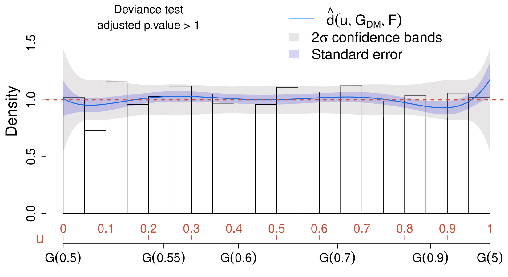 Figure 1
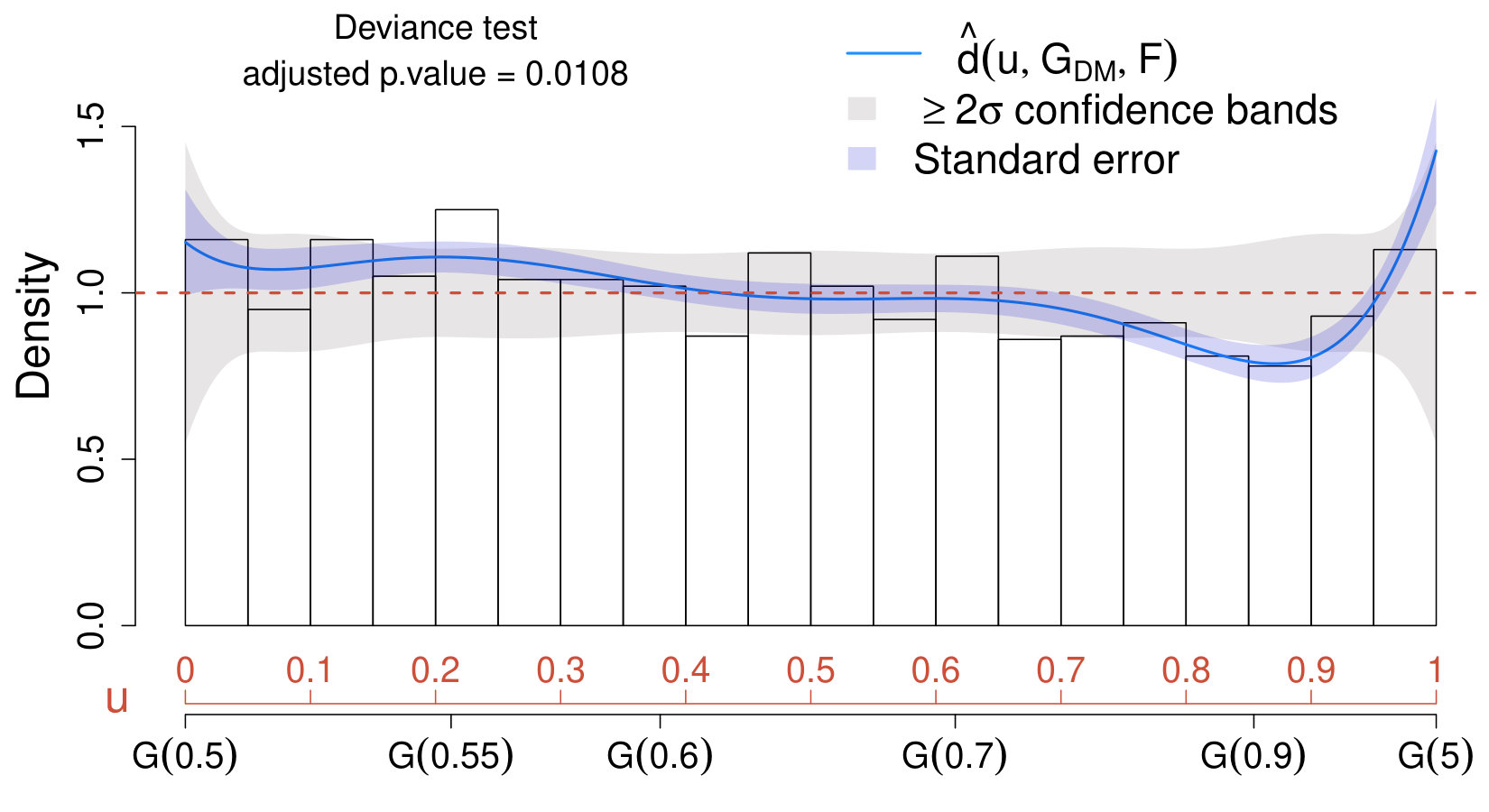 Figure 2
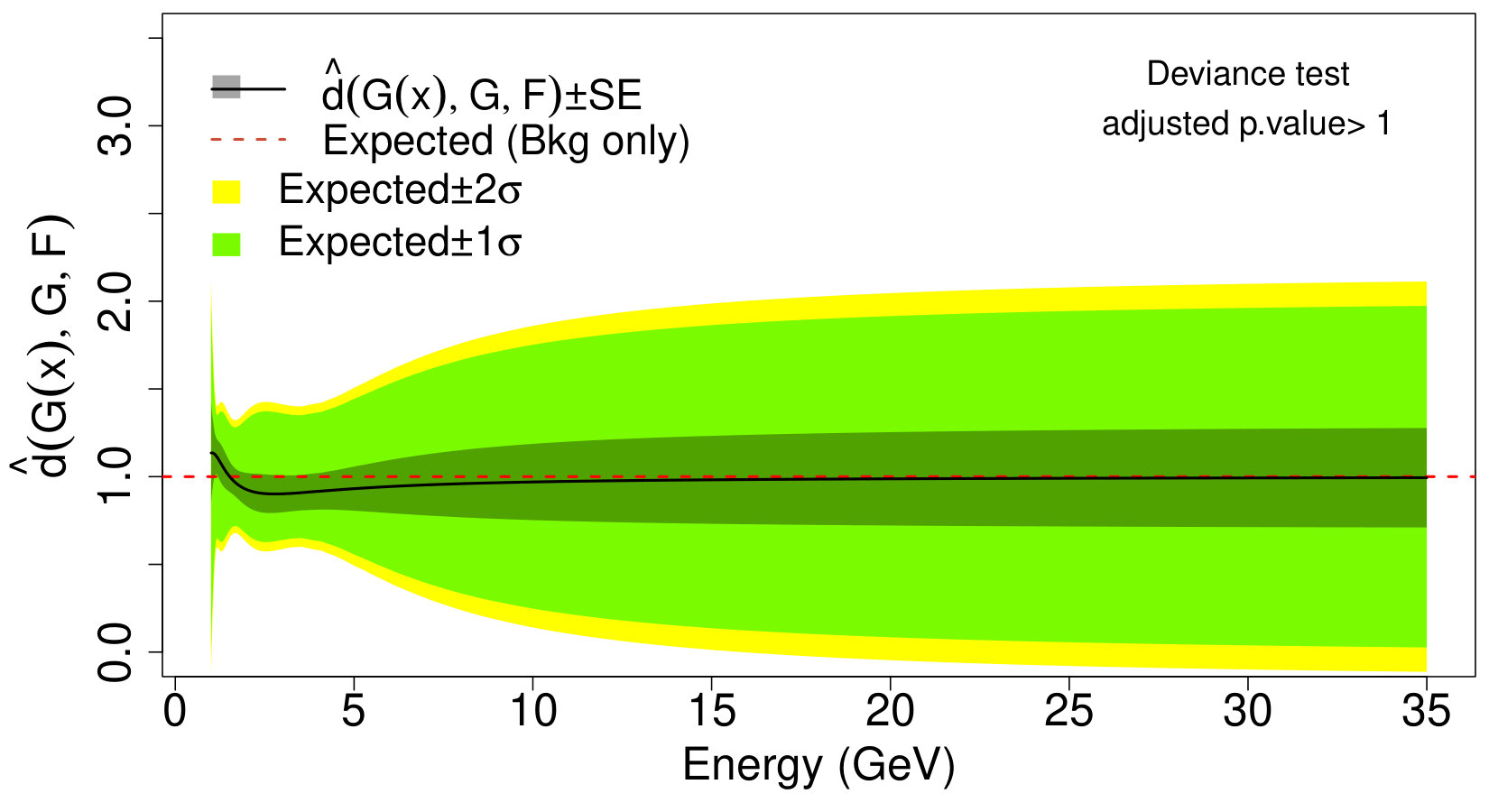 Figure 3
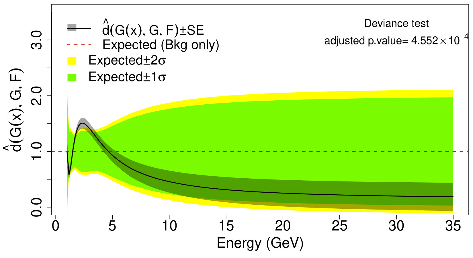 Figure 4
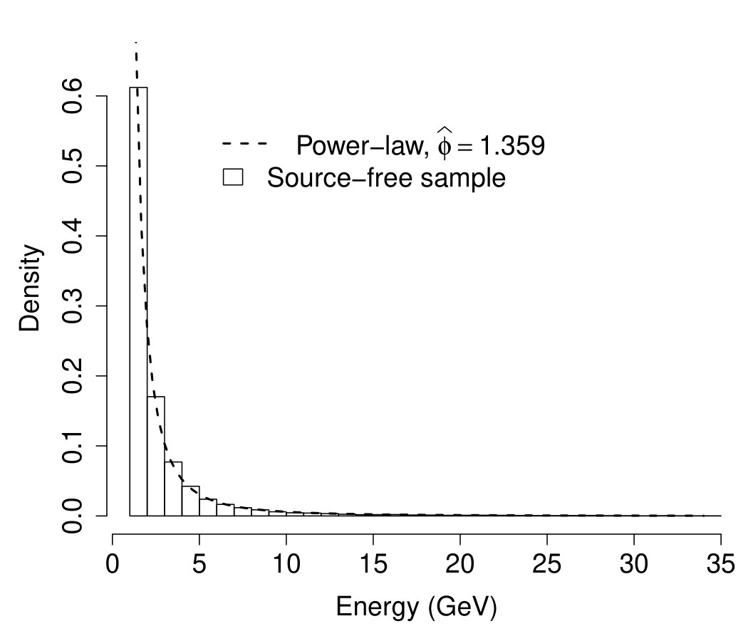 Figure 5
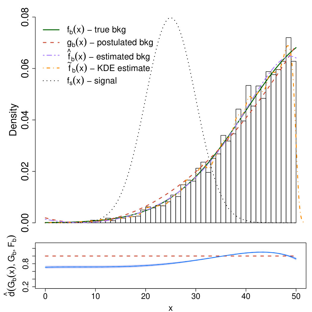 Figure 1
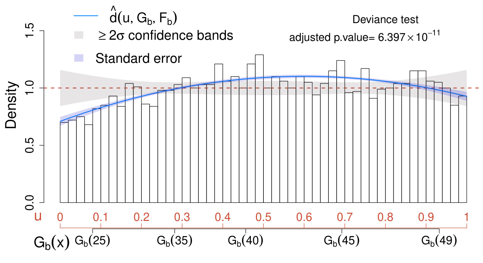 Figure 2
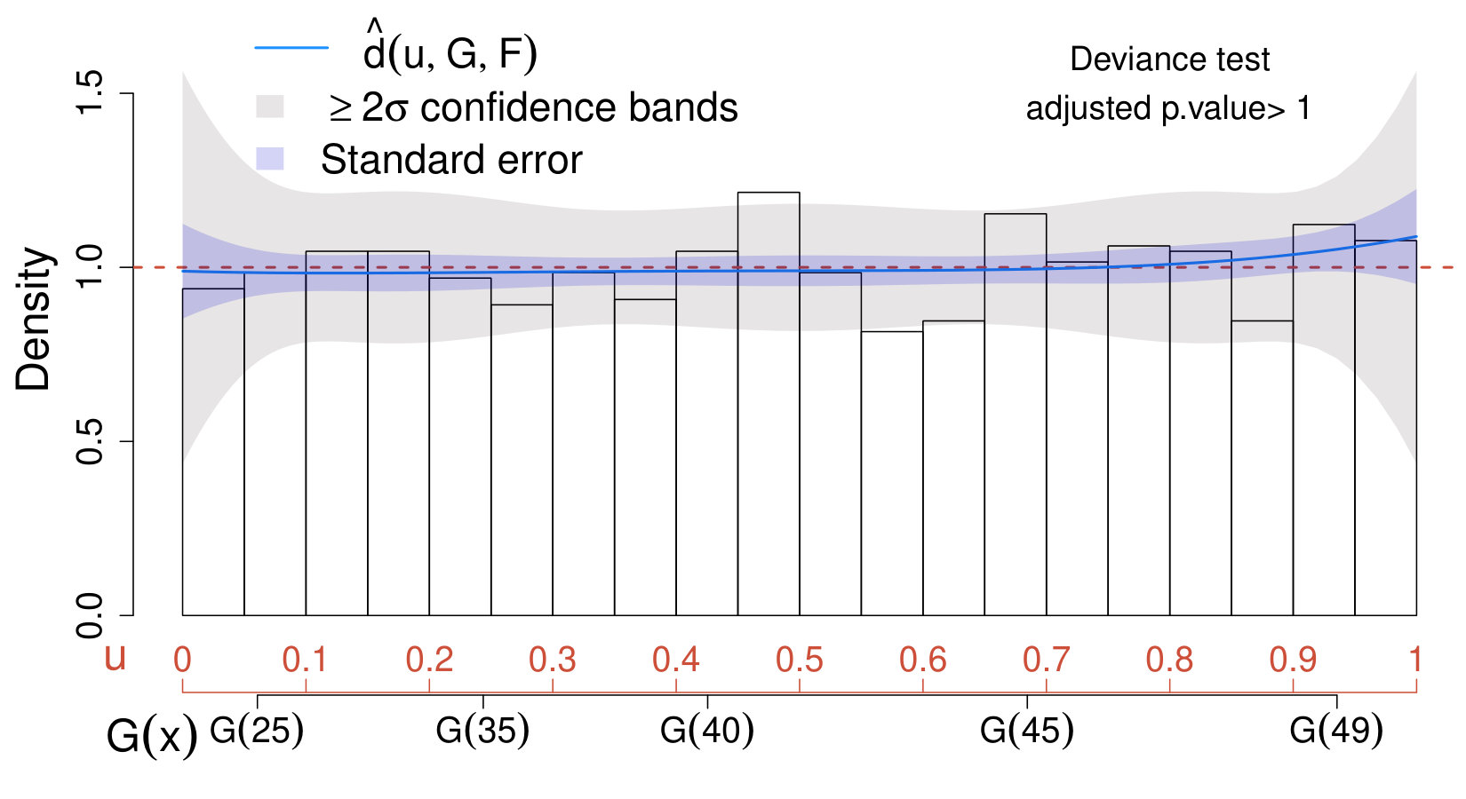 Figure 3
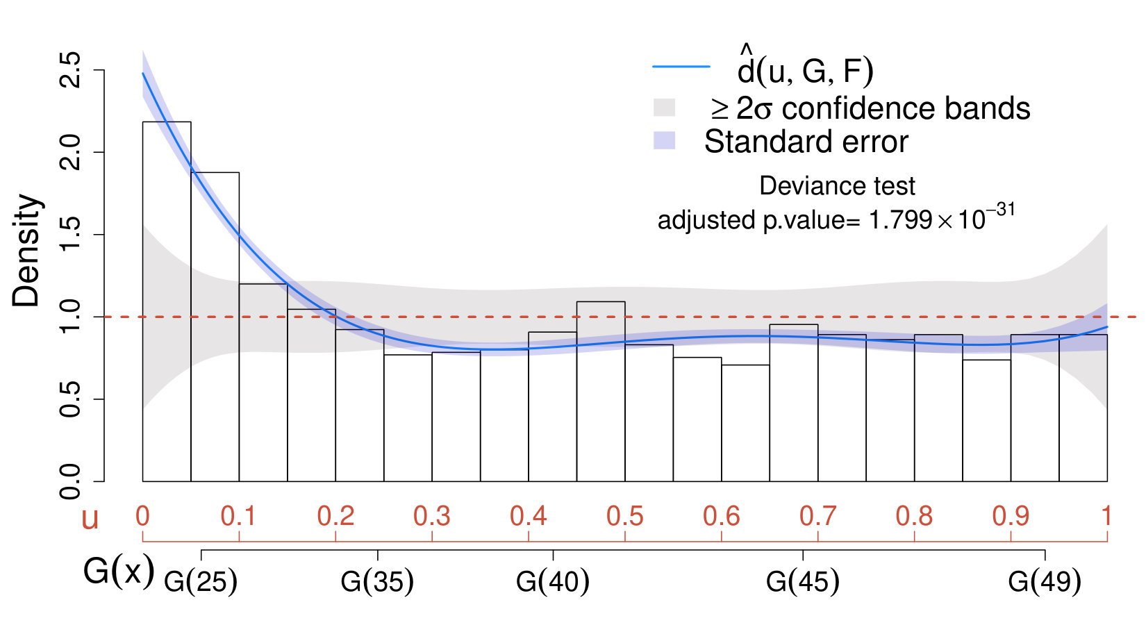 Figure 3
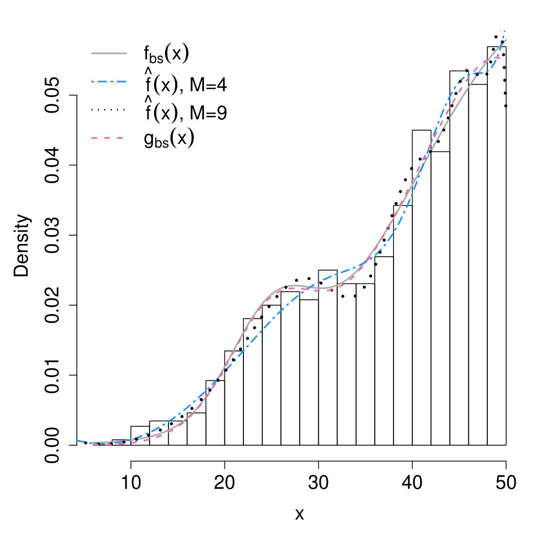 Figure 4
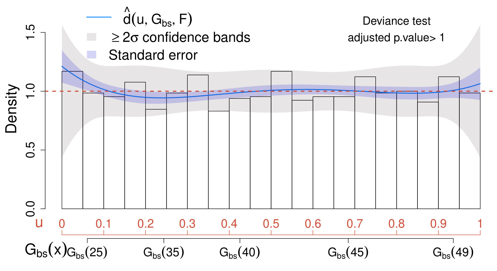 Figure 5
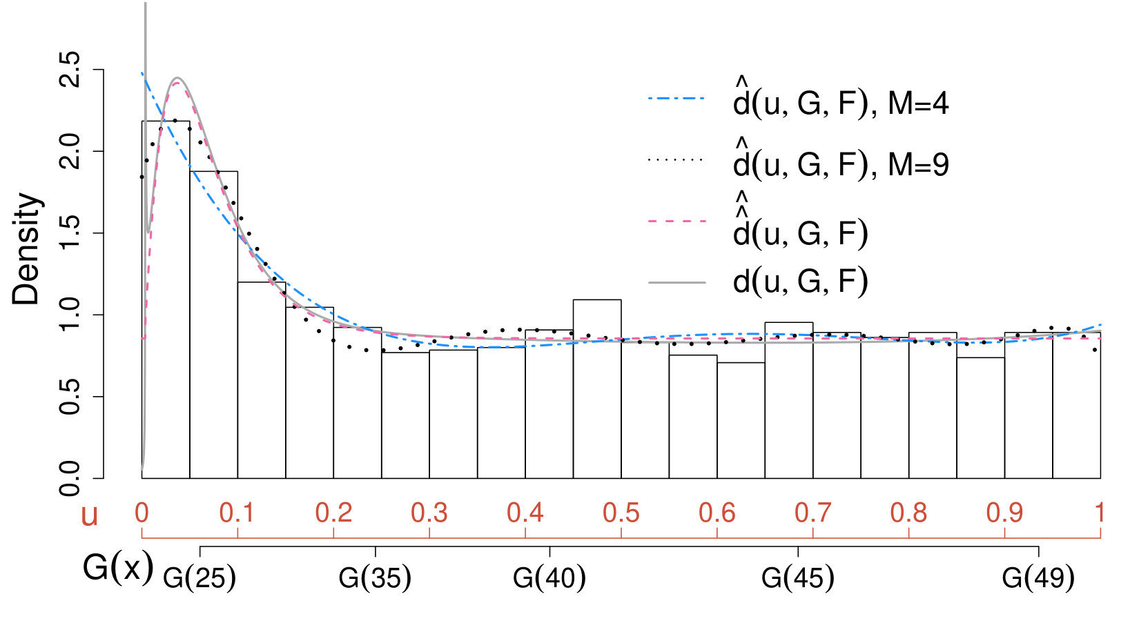 Figure 5
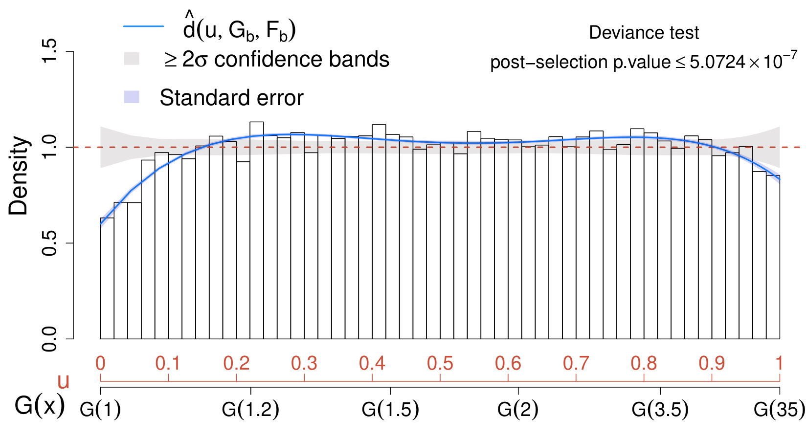 Figure 6
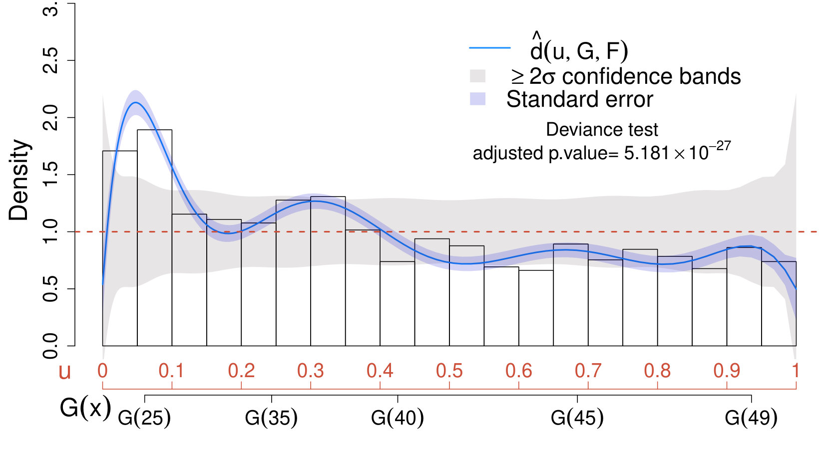 Figure 6
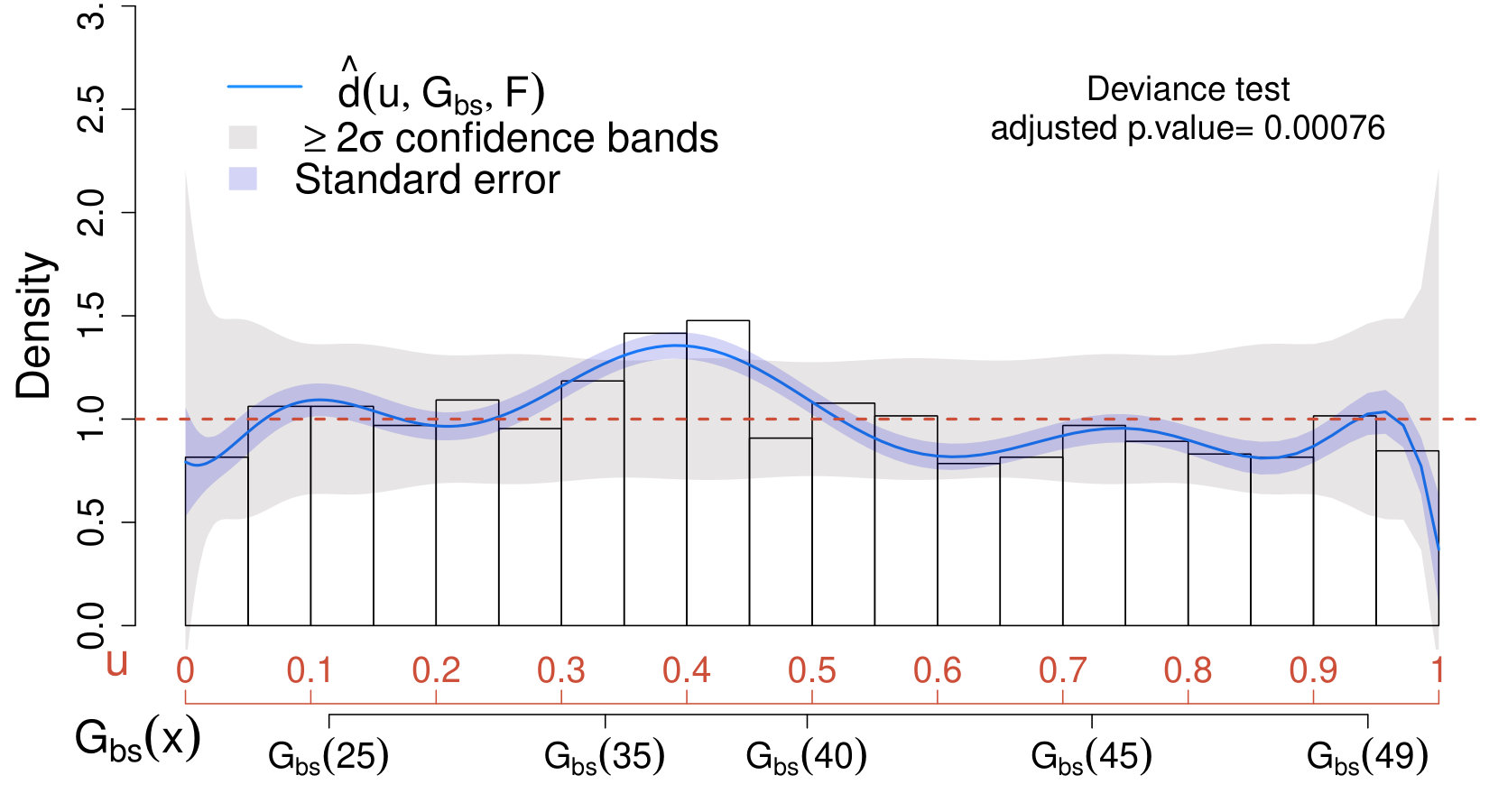 Figure 6
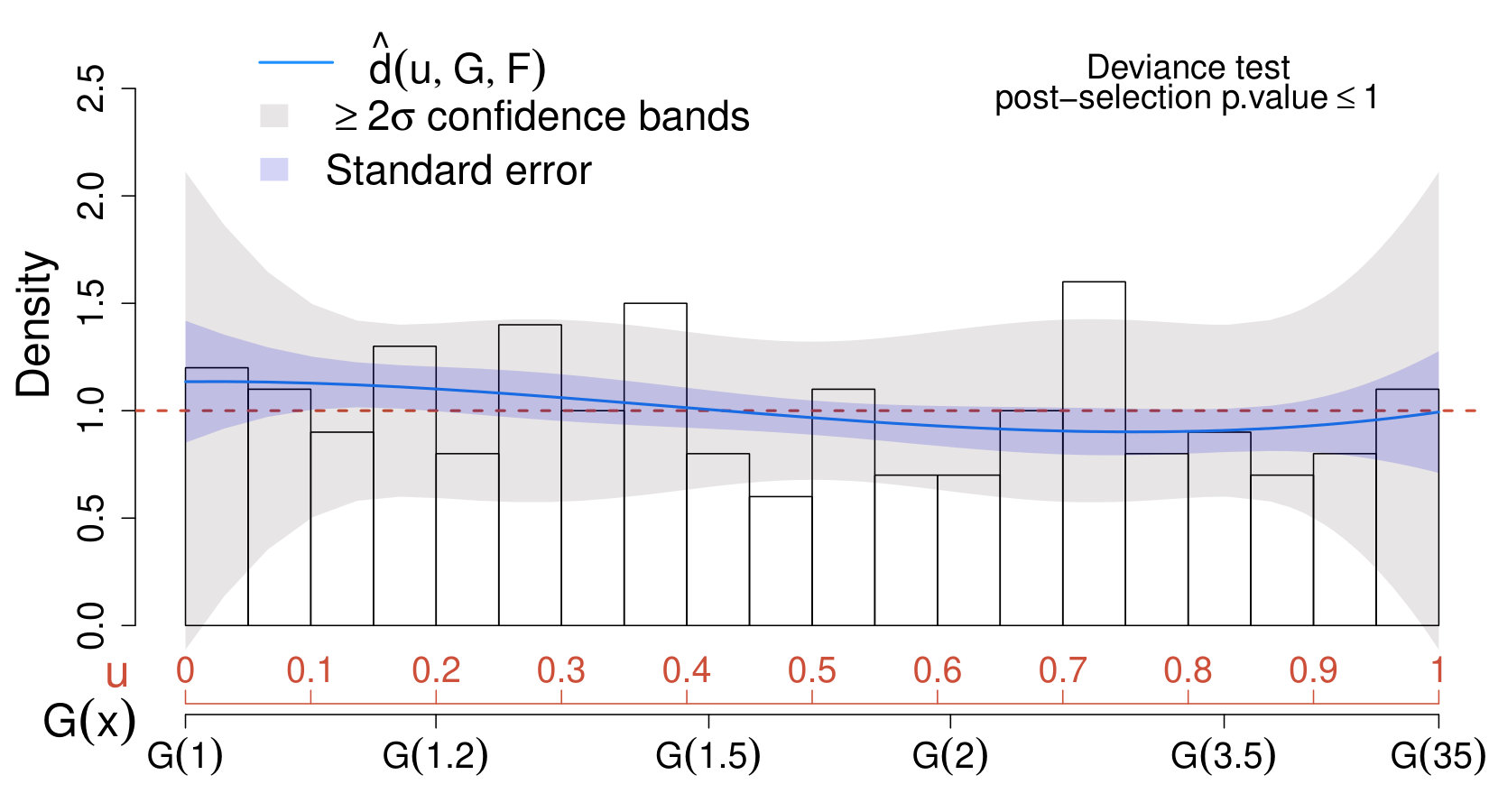 Figure 7
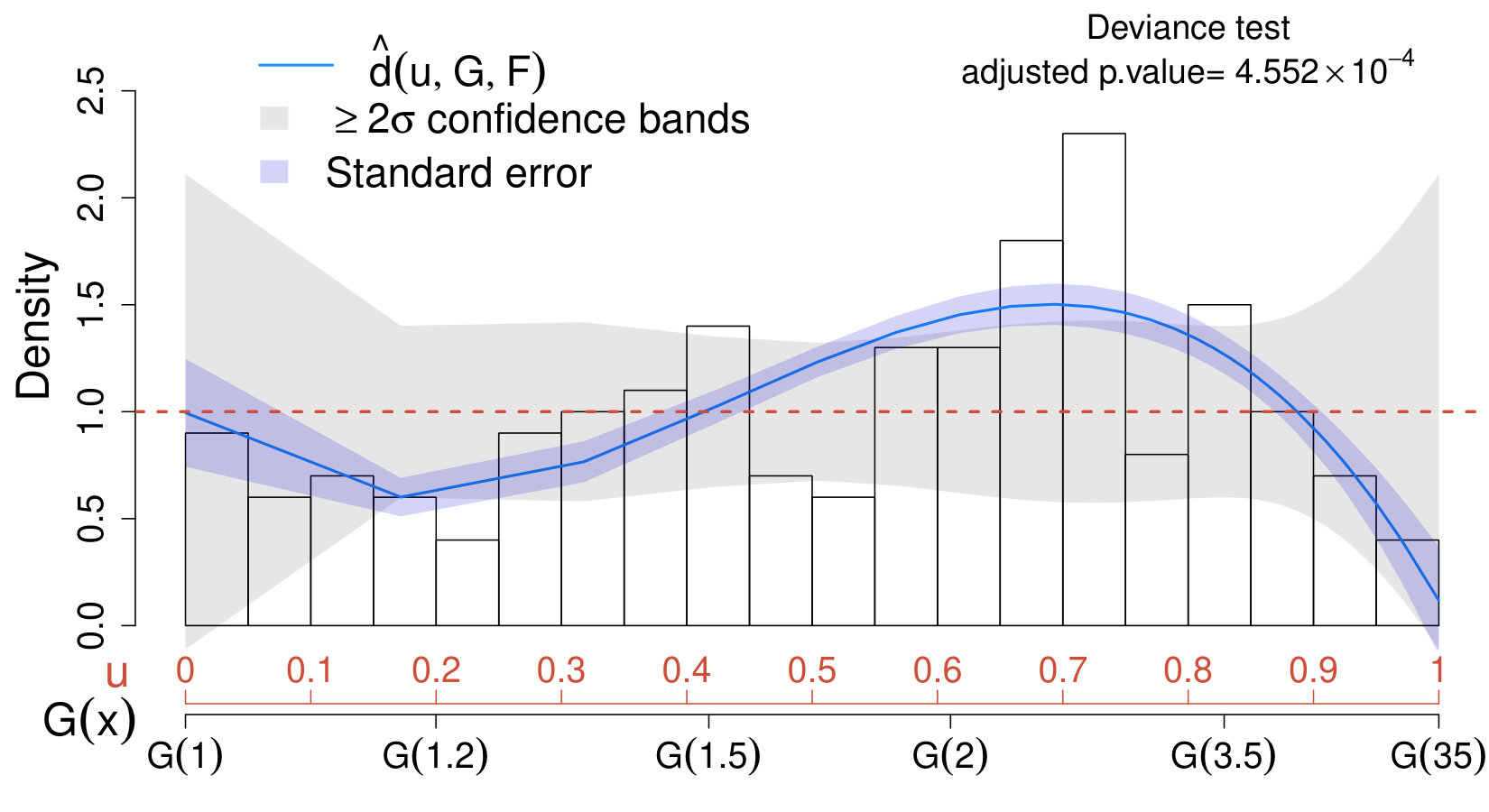 Figure 7
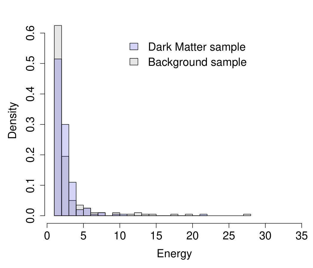 Figure 8
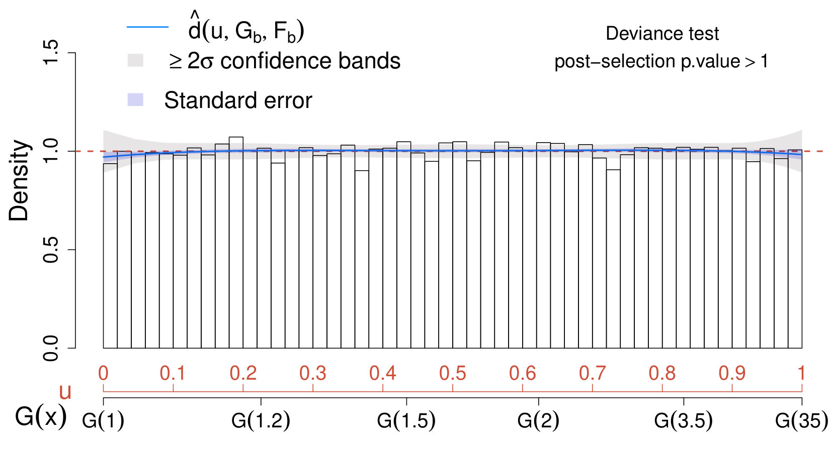 Figure 88
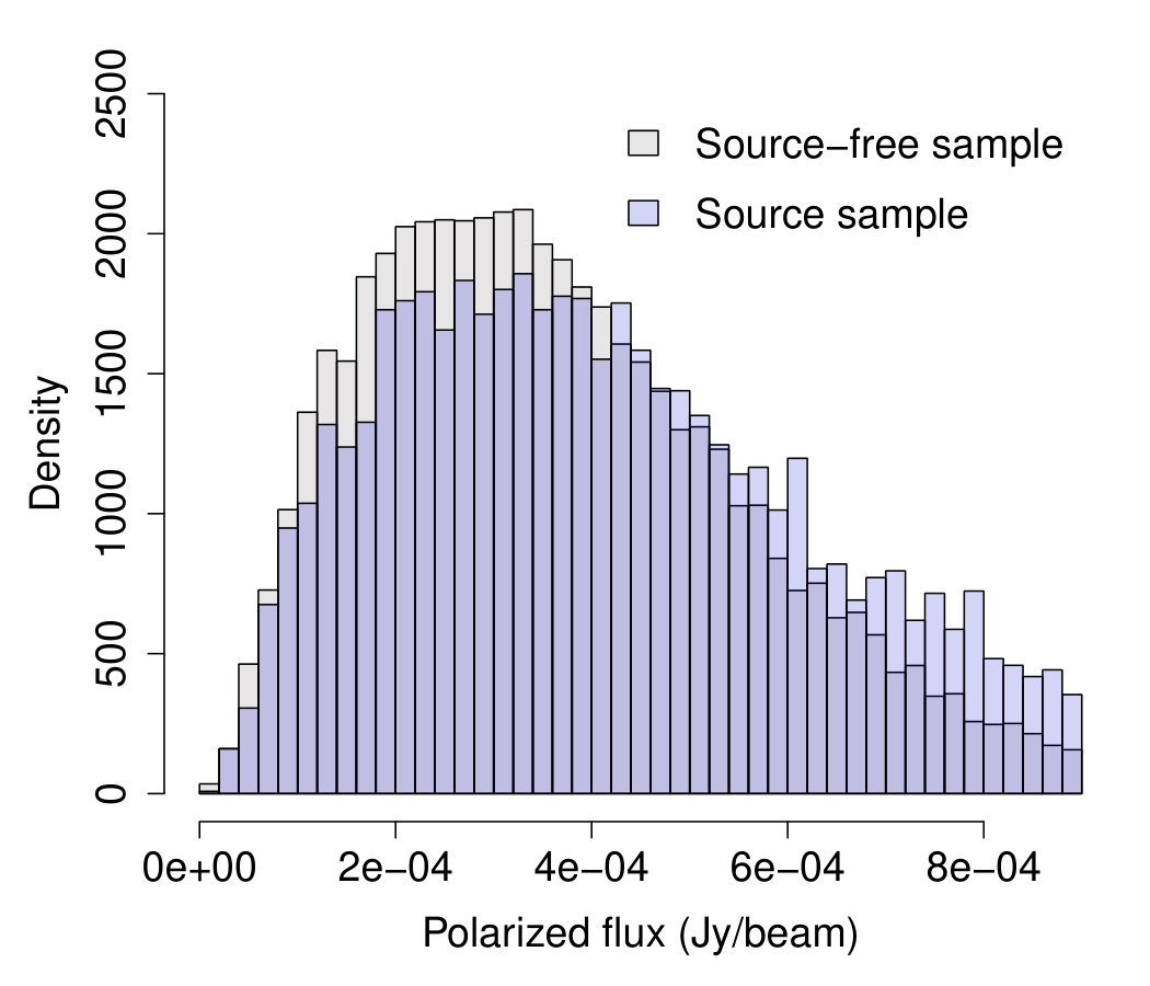 Figure 20
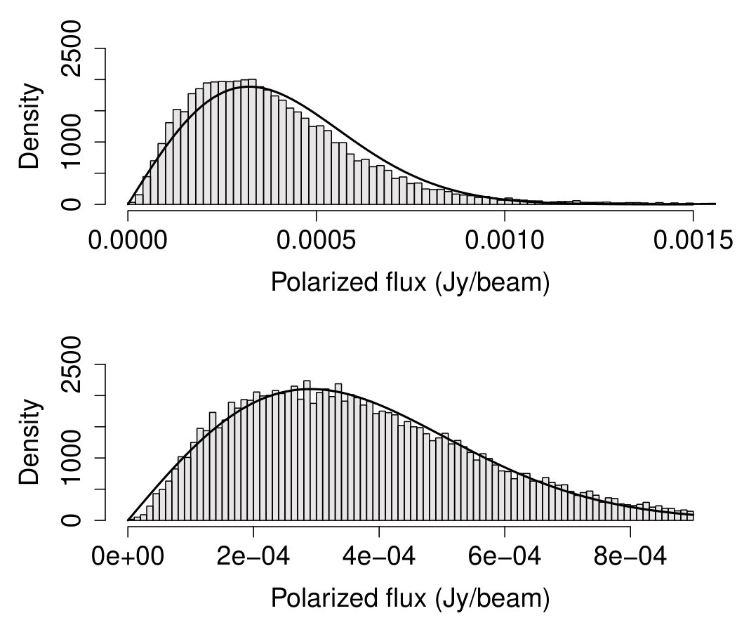 Figure 21
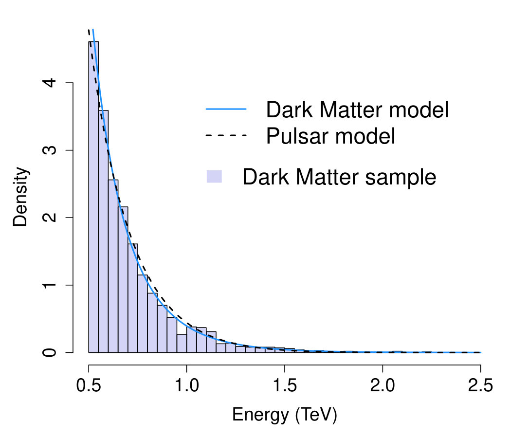 Figure 22
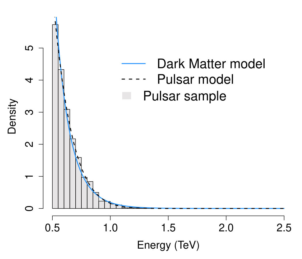 Figure 23
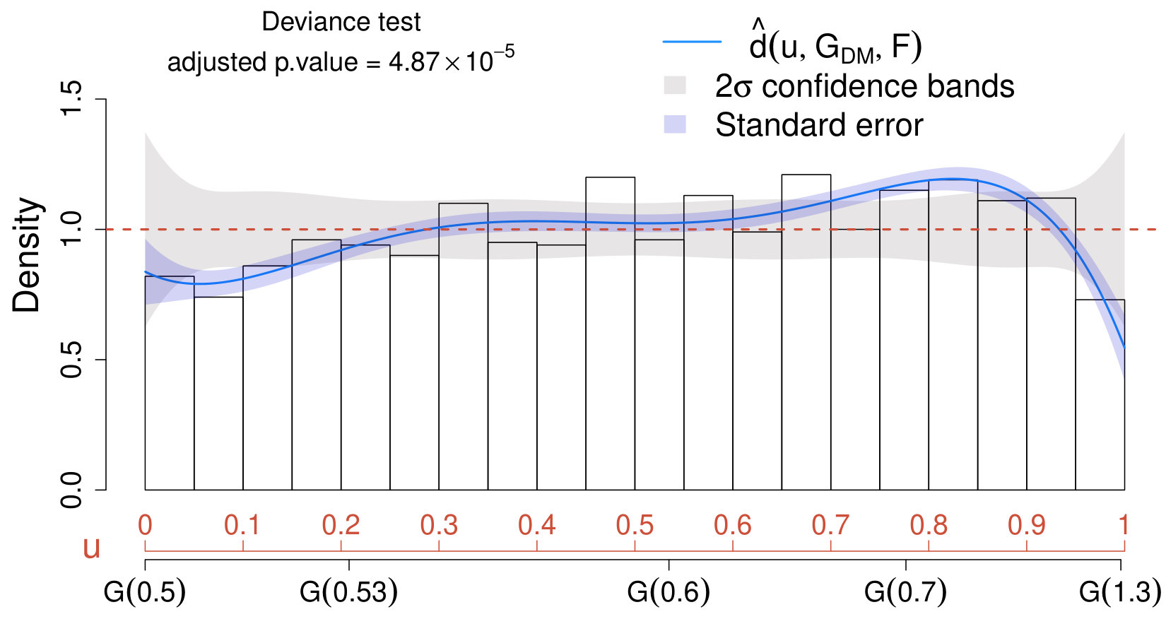 Figure 24
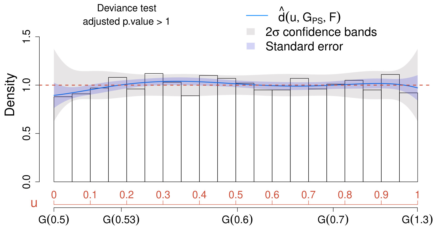 Figure 25
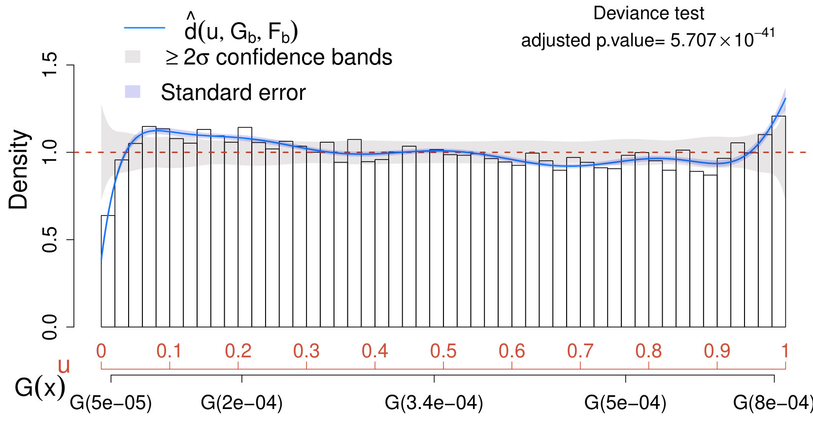 Figure 26
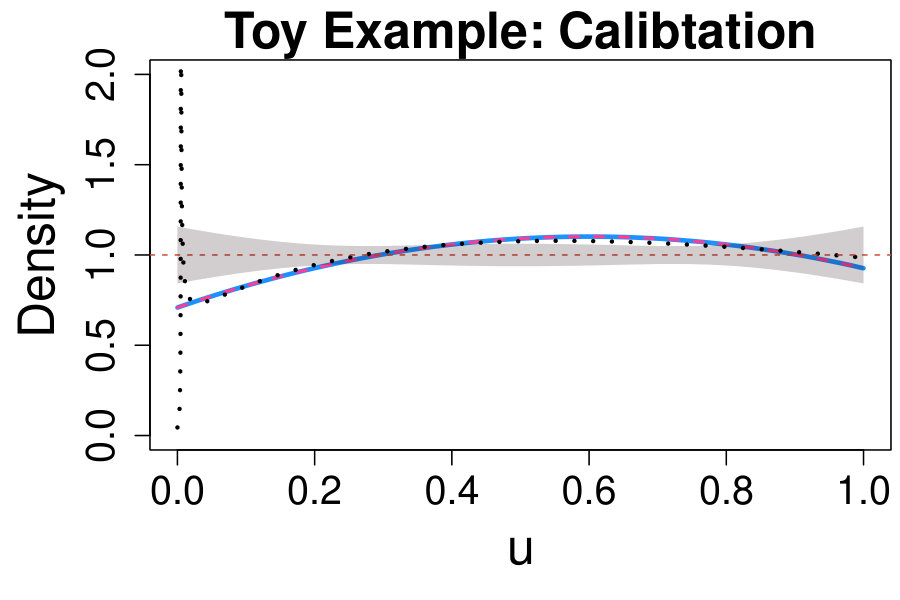 Figure 27
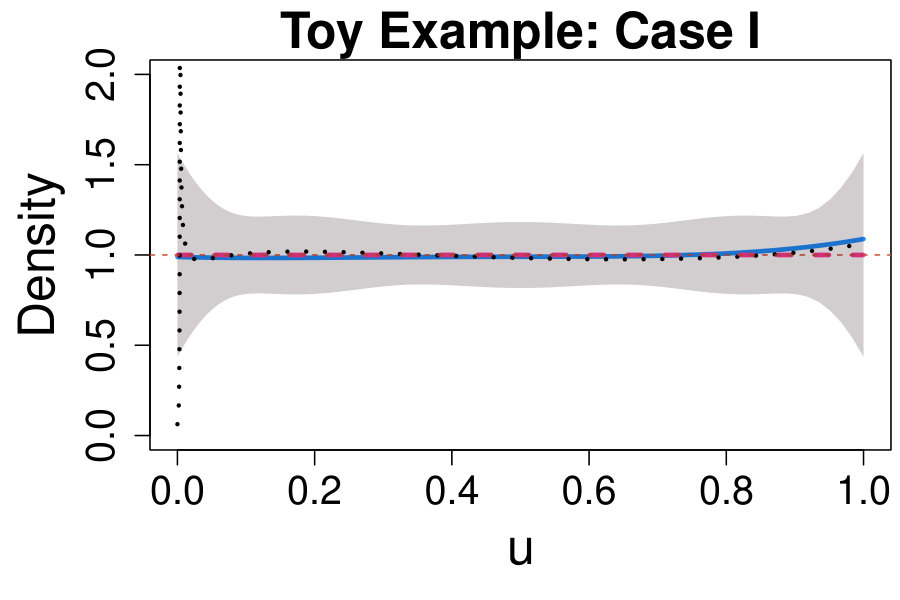 Figure 28
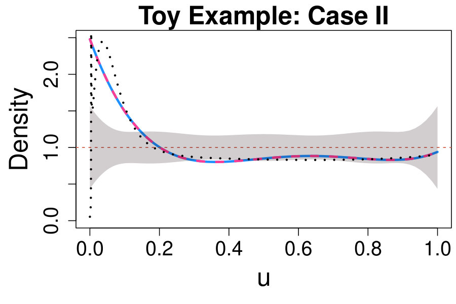 Figure 29
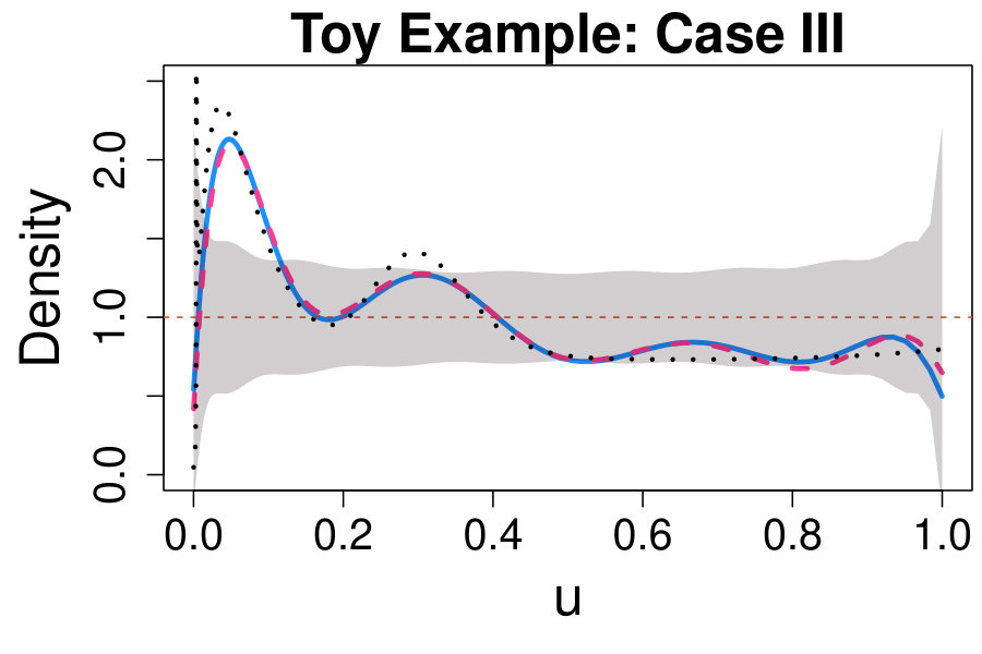 Figure 30
 Figure 31
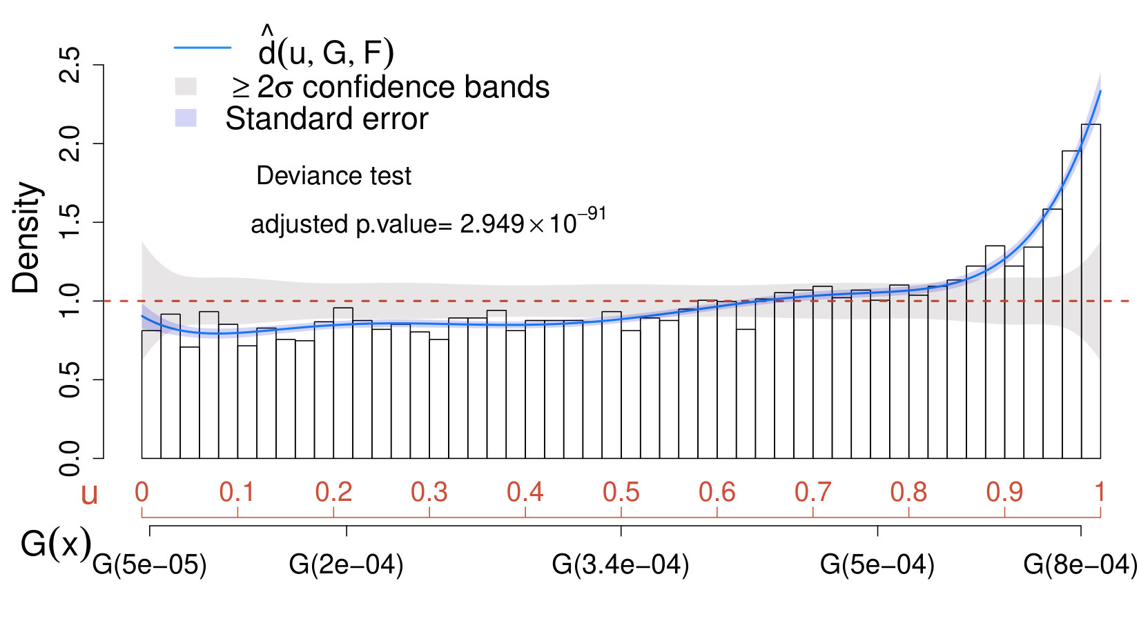 Figure 32
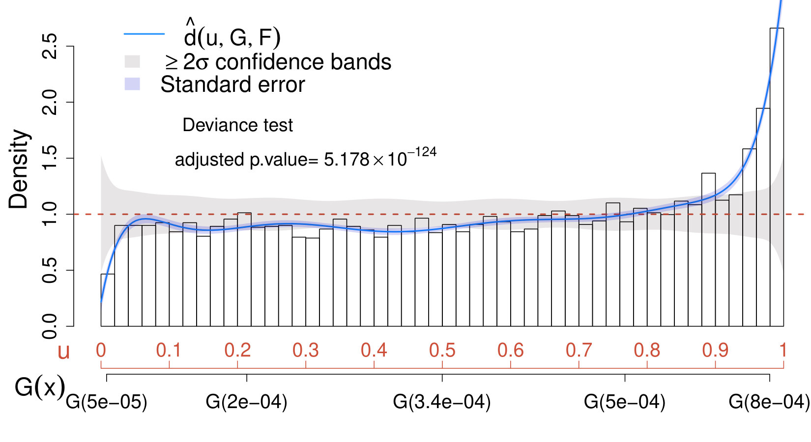 Figure 33
| Goodness-of-fit test p-values | Two-samples test p-values | ||||
| Sample | Anderson-Darling | Cramer-von Mises | Deviance (adjusted) | Kolmogorov-Smirnov | Wilcoxon Rank Sum |
| Calibration | () | - | - | ||
| Case I | () | 0.9248 | 0.5487 | ||
| Case II | () | ||||
| Case III | () | ||||
| Method | Deviance | Adjusted | ||
|---|---|---|---|---|
| selected | p-values | p-values | ||
| Toy example | Full | |||
| Calibration | Denoised | |||
| Toy example | M=18 | Full | ||
| Case I | Denoised | |||
| Toy example | Full | |||
| Case II | Denoised | |||
| Toy example | Full | |||
| Case III | Denoised |
Peer Reviews
No public reviews on file for this paper yet. If you reviewed it on a platform where reviews are public (OpenReview, ICLR, NeurIPS, ICML), you can paste yours below so the community can read it here.
Code & Models
Videos
No videos yet. Explain this paper in a talk, walkthrough, or lecture? Add one.
Version of
††thanks: The author declares no conflict of interest.
Detecting new signals under background mismodelling
Sara Algeri
School of Statistics, University of Minnesota, Minneapolis (MN), 55455, USA
Abstract
Searches for new astrophysical phenomena often involve several sources of non-random uncertainties which can lead to highly misleading results. Among these, model-uncertainty arising from background mismodelling can dramatically compromise the sensitivity of the experiment under study. Specifically, overestimating the background distribution in the signal region increases the chances of missing new physics. Conversely, underestimating the background outside the signal region leads to an artificially enhanced sensitivity and a higher likelihood of claiming false discoveries. The aim of this work is to provide a unified statistical strategy to perform modelling, estimation, inference, and signal characterization under background mismodelling. The method proposed allows to incorporate the (partial) scientific knowledge available on the background distribution and provides a data-updated version of it in a purely nonparametric fashion without requiring the specification of prior distributions on the unknown parameters. Applications in the context of dark matter searches and radio surveys show how the tools presented in this article can be used to incorporate non-stochastic uncertainty due to instrumental noise and to overcome violations of classical distributional assumptions in stacking experiments.
pacs:
02.30.Nw,02.70.Rr,03.65.Db,06.20.Dk,07.05.Kf,12.40.Ee,12.60.-i,14.80.Cp ,98.70.Vc.
I Introduction
When searching for new physics, a discovery claim is made if the data collected by the experiment provides sufficient statistical evidence in favor of the new phenomenon. If the background and signal distributions are specified correctly, this can be done by means of statistical tests of hypothesis, upper limits and confidence intervals.
The problem. In practice, even if a reliable description of the signal distribution is available, providing accurate background models may be challenging, as the behavior of the sources which contribute to it is often poorly understood. Some examples include searches for nuclear recoils of weakly interacting massive particles over electron recoils backgrounds aprile18 , agnese18 , searches for gravitational-wave signals over non-Gaussian backgrounds from stellar-mass binary black holes smith18 , and searches for a standard model-like Higgs boson over prompt diphoton production CMS18 .
Unfortunately, model uncertainty due to background mismodelling can significantly compromise the sensitivity of the experiment under study. Specifically, overestimating the background distribution in the signal region increases the chances of missing new physics. Conversely, underestimating the background outside the signal region leads to an artificially enhanced sensitivity, which can easily result in false discovery claims. Several methods have been proposed in literature to address this problem [e.g., yellin, , Priel, , dauncey, ]. However, to the best of the author’s knowledge, none of the methods available provides a unified strategy to (i) assess the validity of existing models for the background, (ii) fully characterize the background distribution, (iii) perform signal detection even if the signal distribution is not available, (iv) characterize the signal distribution, and (v) detect additional signals of new unexpected sources.
Goal. The aim of this work is to integrate modelling, estimation, and inference under background mismodelling and provide a general statistical methodology to perform of (i)-(v). As a brief overview, given a source-free sample and the (partial) scientific knowledge available on the background distribution, a data-updated version of it is obtained in a purely nonparametric fashion without requiring the specification of prior distributions on the unknown parameters. At this stage, a graphical tool is provided in order to assess if and where significant deviations between the true and the postulated background distributions occur. The “updated” background distribution is then used to assess if the distribution of the data collected by the experiment deviates significantly from the background model. Also in this case, it is possible to assess graphically how the data distribution deviates from the expected background model. If a source-free sample is available, or if control regions can be identified, the solution proposed does not require the specification of a model for the signal; however, if the signal distribution is known (up to some free parameters), the latter can be used to further improve the accuracy of the analysis and to detect the signals of unexpected new sources. Finally, the method can be easily adjusted to cover situations in which a source-free sample or control regions are not available, the background is unknown, or incorrectly specified, but a functional form of the signal distribution is known.
The key of the solution. The statistical methodologies involved rely on the novel LP approach to statistical modelling first introduced by Mukhopadhyay and Parzen in 2014 LPapproach . As it will become clearer later on in the paper, the letter L typically denotes robust nonparametric methods based on quantiles, whereas P stands for polynomials [ksamples, , Supp S1]. This approach allows the unification of many of the standard results of classical statistics by expressing them in terms of quantiles and comparison distributions and provides a simple and powerful framework for statistical learning and data analysis. The interested reader is directed to LPmode , LPBayes , LPtime , LPFdr , LPdec and references therein, for recent advancements in mode detection, nonparametric time series, goodness-of-fit on prior distributions, and large-scale inference using an LP approach.
Organization. Section II is dedicated to a review of the main constructs of LP modelling. Section III highlights the practical advantages offered by modelling background distributions using an LP approach. Section IV introduces a novel LP-based framework for statistical inference. Section V outlines the main steps of a data-scientific approach for signal detection and characterization. In Section VI, the methods proposed are applied in the context of dark matter searches where the goal is to distinguish -ray emissions due to dark matter from those due to pulsars. In Section VII, the tools discussed are applied to a simulation of the Fermi Large Area Telescope -ray telescope and it is shown how upper limits and Brazil plots can be constructed by means of comparison distributions. Section VIII is dedicated to model-denoising. Section IX presents an application to data from the NVSS astronomical survey and discusses a simple approach to assess the validity of distributional assumptions on the polarized intensity in stacking experiments. A discussion of the main results and extensions is proposed in Section X.
II LP Approach to Statistical Modelling
The LP Approach to Statistical Modelling [LPapproach, ] is a novel statistical approach which provides an ideal framework to simultaneously assess the validity of the scientific knowledge available and fill the gap between the initial scientific belief and the evidence provided by the data. Sections II.1, II.2 and II.3 below introduce the LP modelling framework, whereas Section III discusses how the problem of background mismodelling can be formulated under this paradigm.
II.1 The skew-G density model
Let be a continuous random variable with cumulative distribution function (cdf) and probability density function (pdf) . Since is the true distribution of the data, it is typically unknown. However, suppose a suitable cdf is available, and let be the respective pdf. In order to understand if is a good candidate for , it is convenient to express the relationship among the two in a concise manner.
The skew-G density model [LPapproach, , LPmode, ] is a universal representation scheme which allows to express any pdf as
[TABLE]
where is called comparison density manny2 and it is such that
[TABLE]
with and denoting the “postulated” quantile function of . The comparison density is the pdf of the random variable ; whereas, its cdf is given by
[TABLE]
and it is called comparison distribution.
Practical remarks. Equations (2) and (3) are of fundamental importance to understand the power of a statistical modelling approach based on the comparison density. Specifically, allows to “connect” any given pdf to the true pdf through the quantile transformation of . Furthermore, if and only if for all , i.e., is uniformly distributed over the interval . Whereas, if , models the departure of the true density from the postulated model . Consequently, an adequate estimate of , not only leads to an estimate of the true based on (1), but it also allows to identify the regions where deviates substantially from .
II.2 LP skew-G series representation
Denote with the Hilbert space of square integrable functions on the unit interval with respect to the measure . A complete, orthonormal basis of functions in can be constructed considering powers of , i.e., and adequately orthonormalized via Gram-Schmidt procedure LPmode . The resulting bases can equivalently be expressed as normalized shifted Legendre Polynomials,111Classical Legendre polynomials are defined over ; here, their “shifted” counterpart over the range is considered. The first three normalized shifted Legendre polynomials are: , , , etc. namely , with .
Under the assumption that (2) is a square integrable function on , i.e., , we can then represent via a series of polynomials, i.e.,
[TABLE]
with coefficients . The representation in (4) is called LP skew-G series representation [LPmode, ].
II.3 LP density estimate
Let be a sample of independent and identically distributed (i.i.d.) observations from . Observations from are given by . The coefficients in (4) can then be estimated via
[TABLE]
Aternatively, in virtue of (3), the estimates can also be specified as
[TABLE]
where and denote the empirical distribution of the samples and , respectively.
The moments of the are
[TABLE]
where and . When , the equalities in (7) reduce to
[TABLE]
for all . Derivations of (7) and (8) are discussed in Appendix A.
If (4) is approximated by the first terms,222Recall that the first normalized shifted Legendre polynomial is . an estimate of the comparison density is given by
[TABLE]
with variance
[TABLE]
See Appendix B for more details on the derivation of (10). Finally, the standard error of corresponds the square root of (10), with and estimated by their sample counterpart, i.e.,
[TABLE]
Finally, in virtue of the skew-G density model in (1) we can estimate as
[TABLE]
Since each is a polynomial function of the random variable , each estimate can be expressed as a linear combination of the first sample moments of , e.g.,
[TABLE]
where , . Therefore, the truncation point can be interpreted as the order of the highest moment considered to characterize the distribution of . (The reader is directed to Section IV.3 for a discussion on the choice of .)
II.4 The bias variance trade-off
In order to understand how good (9) is in estimating we consider the Mean Integrated Squared Error (MISE) of , i.e.,
[TABLE]
where the first term in (13) corresponds to the integral of the (10) over ; whereas the second term corresponds to the Integrated Squared Bias (IBS), i.e,
[TABLE]
Interestingly, the latter can also be specified as
[TABLE]
(see derivations in Appendix B). The first term on the right hand side of (15) is particularly important in understanding the role played by in obtaining a reliable estimate of . Specifically, the closer is to the lower the bias of and in (11).
Practical remarks. Equation (13) implies that larger values of do not necessarily lead to better estimates of . Specifically, when , the first term in (13) tends to zero. However, for large values of , more and more terms to contribute to it and thus increasing may lead to a substantial inflation of the variance in (10). Conversely, the bias is not affected by sample size and it can be controlled by either choosing sufficiently close to (see (15)) and/or increasing while preserving a good bias-variance trade-off.
Further remarks. Equation (6) implies that the estimator in (9) relies on the empirical distribution of the sample observed by means of the estimates. Therefore, an estimator of the comparison density based entirely on the empirical cdf can be expressed by setting in (9). However, as discussed in this section, while this would reduce the bias, it would also icrease the variance drastically. Therefore, for , the estimator in (9), not only leads to a reduction of the variance but, in virtue of (15), its bias is mitigated when the postulated model is sufficiently close to the true pdf of the data .
III Data-driven corrections for misspecified background models
Let be a sample of observations from control regions or the result of Monte Carlo simulations, where we expect no signal to be present. Hereafter, we refer to as the source-free sample. Therefore, can be used to “learn” the unknown pdf of the background, namely , and obtain an estimate for it via (11).
Despite the true background model being unknown, suppose that a candidate pdf, namely , is available. The candidate model can be specified from previous experiments or theoretical results or can be obtained by fitting specific functions (e.g., polynomial, exponential, etc.) to . If does not provide an accurate description of , the sensitivity of the experiment can be strongly affected.
Consider, for instance, a source-free sample of observations whose true (unknown) distribution corresponds to the tail of a Gaussian with mean and width over the range , i.e.,
[TABLE]
with k_{fb}=\int_{0}^{50}e^{-\frac{1}{2}\bigl{(}\frac{x-55}{15}\bigl{)}^{2}}\partial x. Suppose that a candidate model for the background is obtained by fitting a second-degree polynomial on the source-free sample and adequately normalizing it in order to obtain a proper pdf, i.e.,
[TABLE]
with . For illustrative purposes, assume that the distribution of the signal is a Gaussian centered at , with width and pdf
[TABLE]
with k_{fs}=\int_{0}^{50}e^{-\frac{1}{2}\bigl{(}\frac{x-25}{4.5}\bigl{)}^{2}}\partial x. The histogram of the source-free sample along with (16)-(18) is shown in Fig. 1. At the higher end of the spectrum, the postulated background (red dashed line) underestimates the true background distribution (green solid line). As a result, using (17) as background model increases the chance of false discoveries in this region. Conversely, at the lower end of the spectrum, underestimates , reducing the sensitivity of the analysis. For the sake of comparison, a Kernel density estimate (orange dot-dashed line) has been computed by selecting the bandwidth parameter as recommended in sheater . The latter exhibits substantial bias at the boundary and appears to overfit the data sample.
It is important to point out that, the discrepancy of from is typically due to the fact that the specific functional form imposed (in our example, a second-degree polynomial) is not adequate for the data. Thus, changing the values of the fitted parameters (or assigning priors to them) is unlikely to solve the problem. However, it is possible to “repair” and obtain a suitable estimate of by means of (11). Specifically, can be estimated via
[TABLE]
where is the comparison density estimated via (9) on the sample , whereas and are the true and the postulated background distributions, with pdfs as in (16) and (17), respectively.
In our example, choosing (see Section IV.3), we obtain
[TABLE]
where and are the first and second normalized shifted Legendre polynomials evaluated at . Notice that, by combining (19) and (20), we can easily write the background model using of a series of shifted Legendre polynomials. This may be especially useful when dealing with complicated likelihoods and for which a functional form is difficult to specify.
The upper panel of Fig. 1 shows that the “calibrated” background model in (19) as a purple dot-dashed line and matches almost exactly the true background density in (16) (green solid line). The plot of in the bottom panel of Fig. 1 provides important insights on the deficiencies of (17) as a candidate background model. Specifically, the magnitude and the direction of the departure of from one corresponds to the estimated departure of from for each value of . Therefore, if is below one in the region where we expect the signal to occur, using in place of increases the sensitivity of the analysis. Conversely, if is above one outside the signal region, the use of instead of prevents from false discoveries.
Notice that in this article we only consider continuous data. In this respect, the goal is to learn the model of the background considered as a continuum and no binning is applied. Therefore, the histograms presented here are only a graphical tool used to display the data distribution and are not intended to represent an actually binning of the data.
IV LP-based inference
When discussing the skew-G density model in (1), we have witnessed that if for all . Additionally, the graph of provides an exploratory tool to understand the nature of the deviation of from . This section introduces a novel inferential framework to test the significance of the departure of from . Specifically, our goal is to test the hypotheses
[TABLE]
First, an overall test, namely the deviance test, is presented. The deviance test assesses if deviates significantly from anywhere over the range of considered. Second, adequate confidence bands are constructed in order to assess where significant departures occur.
IV.1 The deviance test
Recall that the coefficients in (4) specify as . Consequently, by orthogonality of the polynomials and , when in (21) is true all the coefficients are equal to zero, including the first of them. We can then quantify the departure of from one by means of the deviance statistics LPFdr which specifies as . If the deviance is equal to zero, we may expect that is approximately equivalent to ; hence, we test
[TABLE]
by means of the test statistic
[TABLE]
It can be shown LPmode that, as
[TABLE]
where denotes convergence in distribution, and thus, under , is asymptotically -distributed. Hence, an asymptotic p-value for (22) is given by
[TABLE]
where is the value of observed on the data.
Practical remarks. Notice that in (22) implies in (21). Similarly, in (21) implies in (22); however, the opposite is not true in general since there may be some non-zero coefficients for . Therefore, even when choosing small may lead to conservative, but yet valid, inference.
IV.2 Confidence bands
The estimator in (9) only accounts for the first terms of the polynomial series in (4). Therefore, is a biased estimator of . Specifically, as discussed in Section II.4, the integrated bias is given by , whereas, as show in Appendix B, the bias at a given point is given by . It follows that, when the bias is large, confidence bands based on are shifted away from the true density .
Despite the bias cannot be easily quantified in the general setting, it follows from (8) that, when in (21) (and consequently in (22)) is true, both the bias at a point and the integrated bias are equal to zero. Thus, we can exploit this property to construct reliable confidence bands under the null. Specifically, the goal is to identify , such that
[TABLE]
where is the desired significance level.333In astrophysics, the statistical significance is often expressed in terms of number of -deviations from the mean of a standard normal, namely . For instance, a 2 significance corresponds to , where denotes the cdf of a standard normal.
If the bias determines where the confidence bands are centered, the distribution and the variance of determine their width. As discussed in Section II.3 (see (8)), under in (21), the estimates have mean zero, variance and they are uncorrelated one another. Therefore, when , the standard error of , corresponds to the square root of (10) with and i.e.,
[TABLE]
Additionally, (24) implies that is asymptotically normally distributed, hence
[TABLE]
as , for all , under .
We can then construct approximate confidence bands under which satisfy (26) by means of tube formulae (see [larry, , Ch.5] and PL05 ), i.e.,
[TABLE]
where is the solutions of
[TABLE]
with . If is within the bands in (29) over the entire range , we conclude that there is no evidence that deviates significantly from anywhere over the range considered and at confidence level . Conversely, we expect significant departures to occur in regions where lies outside the confidence bands.
Practical remarks. Notice that, under in (22), the is an unbiased estimator of , regardless of the choice of . This implies that the confidence bands in (29) are only affected by the variance and asymptotic distribution of under .
IV.3 Choice of
The number of estimates considered determines the level of “smoothness” 444 As an anonymous referee correctly pointed out, is always smooth as it is constructed as a series of infinitely differentiable functions. In statistics, however, the word “smoothness” is often used to indicate the flexibility of the estimator considered or, in other words, its degrees of freedom. Often, this is quantified in terms of magnitude of the second derivative of the function considered. Despite the abuse of terminology, throughout the manuscript we will refer to the latter definition of smoothness. of , with smaller values of leading to smoother estimates. The deviance test can be used to select the value which maximizes the sensitivity of the analysis according to the following scheme:
- i.
Choose a sufficiently large value . 2. ii.
Obtain the estimates as in (5). 3. iii.
For :
- calculate the deviance test p-value as in (25), i.e.,
[TABLE]
with . 4. iv.
Choose such that
[TABLE]
IV.3.1 Adjusting for post-selection
As any data-driven selection process, the scheme presented above affects the distribution of (9) and can yield to overly optimistic inference xiaotong , potscher . Despite this aspect being often ignored in practical applications, correct coverage can only be guaranteed if adequate corrections are implemented.
The issues arising in the context of post-selection inference can be interpreted in terms of looks-elsewhere effect gv10 , meJINST where one has to adjust the inference for the fact that, in practice, many different models have been considered and, consequently, many different tests have been conducted for the sake of assessing the goodness of fit.
In our setting, the number of models under comparison is typically small (); therefore, post-selection inference can be easily adjusted by means of Bonferroni’s correction bonferroni35 . Specifically, the adjusted deviance p-value is given by
[TABLE]
where is the value selected via (32), whereas confidence bands can be adjusted by substituting in (29), with satisfying
[TABLE]
Practical remarks. As noted in Section II, the estimate (9) involves the first sample moments of ; therefore, can be interpreted as the order of the highest moment which we expect to contribute in discriminating the distribution of from uniformity. Notice that, in addition to the inflation of the variance of (9), when is large, the computation of normalized shifted Legendre of higher order may face numerical instability (see Section VIII.2). Therefore, as a rule of thumb, is typically chosen . Finally, Steps i-iv aim to select the approximant based on the first most significant moments, while excluding powers of higher order. A further note on model-denoising is given in Section VIII.
V A data-scientific approach to signal searches
The tools presented in Sections II and IV provide a natural framework to simultaneously
- (a)
assess the validity of the postulated background model and, if necessary, update it using the data (Section III);
- (b)
perform signal detection on the physics sample;
- (c)
characterize the signal when a model for it is not available.
Furthermore, if the model for the signal is known (up to some free parameters), it is possible to
- (d)
further refine the background or signal distribution;
- (e)
detect hidden signals from new unexpected sources.
Notice that, since Bonferroni’s correction leads to an upper bound for the overall significance, the resulting coverage will be higher than the nominal one. Alternatively, approximate post-selection confidence bands and inference can be constructed using Monte Carlo and/or resampling methods and repeating the selection process at each replicate.
Tasks (a)-(e) can be tackled in two main phases. In the first phase, the postulated background model is “calibrated” on a source-free sample in order to improve the sensitivity of the analysis and reduce the risk of false discoveries. The second phase focuses on searching for the signal of interest and involves both a nonparametric signal detection stage and a semiparametric stage for signal characterization. Both phases and respective steps are described in details below and summarized in Algorithm 1.
V.1 Background calibration
As discussed in Section III, deviations of from one suggest that a further refinement of the candidate background model is needed. However, as increases, the deviations of from one may become more and more prominent while the variance inflates. Thus, it is important to assess if such deviations are indeed significant. In order address this task, the analysis of Section III can be further refined in light of the inferential tools introduced in Section IV.
For the toy example discussed in Section III, we have seen that overestimates in the signal region and underestimates it at the higher end of the range considered (Fig. 1). We can now assess if any of these deviations are significant by implementing the deviance test in (23)-(25), whereas, to identify where the most significant departures occur, we construct confidence bands under the null model as in (29), i.e., assuming that no “update” of is necessary.
The results are collected in the comparison density plot or CD plot presented in Fig. 2. First, a value has been selected as in (32), and the respective deviance test (adequately adjusted via Bonferroni) indicates that the deviation of from is significant at a significance level (adjusted p-value of ). Additionally, the estimated comparison density in (20) lies outside the confidence bands in the region where the signal specified in (18) is expected to occur. Hence, using (19) instead of (17) is recommended in order to improve the sensibility of the analysis in the signal region.
Important remarks on the CD plot. When comparing different models for the background or when assessing if the data distribution deviates from the model expected when no signal is present, it is common practice to visualize the results of the analysis by superimposing the models under comparison to the histogram of the data observed on the original scale (e.g., upper panel of Fig. 1). This corresponds to a data visualization in the density domain. Conversely, the CD plot (e.g., Fig. 2) provides a representation of the data in the quantile domain, which offers the advantage of connecting the true density of the data with the quantiles of the postulated model (see (2)-(3)). Consequently, the most substantial departures of the data distribution from the expected model are magnified, and those due to random fluctuations are smoothed out (see, also, Section VII.2). Furthermore, the deviance tests and the CD plot together provide a powerful goodness-of-fit tool and exploratory which, conversely from classical methods such as Anderson-Darling anderson and Kolmogorov-Smirnov darling , not only allow to test if the distributions under comparison differ, but they also allow to assess how and where they differ. As a result, the CD plot can be used to characterize the unknown signal distribution (see Section V.2.2) and to identify exclusion regions (e.g., Case I in Section V.2.1).
As an additional advantage, the deviance test appears to enjoy higher detection power than classical approaches. This aspect is highlighted in Table 1 where several methods for goodness of fit or two-samples comparisons are implemented, along with the deviance test, for all the cases discussed in Section V.
Reliability of the calibrated background model. The size of the source-free sample plays a fundamental role in the validity of as a reliable background model. Specifically, the randomness involved in (19) only depends on the estimates. If is sufficiently large, by the strong law of large numbers,
[TABLE]
Therefore, despite the variance of becoming negligible as , one has to account for the fact that leads to a biased estimate of when (see Section II.4). For sufficiently smooth densities, a visual inspection is often sufficient to assess if (and, consequently, ) provides a satisfactory fit for the data, whereas, for more complex distributions the effect of the bias can be mitigated considering larger values of and model-denoising (see Section VIII.1).
V.2 Signal search
V.2.1 Nonparametric signal detection
The background calibration phase allows the specification of a well tailored model for the background, namely , which simultaneously integrates the initial guess, , and the information carried by the source-free data sample. Hereafter, we disregard the source-free data sample and focus on analyzing the physics sample.
Under the assumption that the source-free sample has no significant source contamination, we expect that, if the signal is absent, both the source-free and the physics sample follow the same distribution. Therefore, the calibrated background model, , plays the role of the postulated distribution for the physics sample, i.e., the model that we expect the data to follow when no signal is present; hence, we set .
Let be the (unknown) true pdf of the physics sample which may or may not carry evidence in favor of the source of interest. When no model for the signal is specified, it is reasonable to consider any significant deviation of from as an indication that a signal of unknown nature may be present. In this setting, similarly to the background calibration phase, we can construct deviance tests and CD plots to assess if and where significant departures of from occur. Two possible scenarios are considered – a physics sample which collects only background data (Case I) and a physics sample of observations from both background and signal (Case II).
Case I: background-only. Let be a physics sample of observations whose true (unknown) pdf is equivalent to in (16). We set
[TABLE]
where and are defined as in (17) and (20), respectively. The resulting CD plot and deviance test are reported in the left panel of Fig. 3.
When applying the scheme in Section IV.3 with , none of the values of considered leads to significant results; therefore, for the sake of comparison with Case II below, we choose . Not surprisingly, the estimated comparison density approaches one over the entire range and lies entirely within the confidence bands. This suggests that the true distribution of the data does not differ significantly from the model which accounts only for the background. Similarly, the deviance test leads to very low significance (adjusted p-value ); hence, we conclude that our physics sample does not provide evidence in favor of the new source.
Case II: background + signal. Let be a physics sample of observations whose true (unknown) pdf is equal to in (36)
[TABLE]
with and defined as in (16) and (18) respectively, and . The histogram of the data and the graph of are plotted in Fig. 4. As in Case I, we set as in (35).
The CD plot and deviance test in the right panel of Fig. 3 show a significant departure of the data distribution from the background-only model in (35). The maximum significance of the deviance is achieved at , leading to a rejection of the null hypothesis at a significance level (adjusted p-value). The CD plot shows a prominent peak at the lower end of the spectrum; hence, we conclude that there is evidence in favor of the signal, and we proceed to characterize its distribution as described in Section V.2.2.
V.2.2 Semiparametric signal characterization
The signal detection strategy proposed in Section V.2.1 does not require the specification of a distribution for the signal. However, if a model for the signal is known (up to some free parameters), the analysis can be further refined by providing a parametric estimate of the comparison density and assessing if additional signals from new unexpected sources are present.
Case IIa: background + (known) signal.** ** Assume that a model for the signal, , is given, with being a vector of unknown parameters. Since the CD plot in the right panel of Fig. 3 provides evidence in favor of the signal, we expect the data to be distributed according to the pdf
[TABLE]
where is the calibrated background distribution in (35) and and can be estimated via Maximum Likelihood (ML). Letting and be the ML estimates of and respectively, we specify
[TABLE]
as postulated model. For simplicity, let to be fully specified as in (18); we construct the deviance test and the CD plot to assess if (38) deviates significantly from the true distribution of the data. The scheme in Section IV.3 has been implemented with , and none of the values of considered led to significant results. The CD plot and deviance test for are reported in the upper left panel of Fig. 5. Both the large p-value of the deviance test (adjusted p-value) and the CD plot suggest that no significant deviations occur; thus, (38) is a reliable model for the physics sample.
Moreover, we can use (38) to further refine our or distributions. Specifically, we first construct a semiparametric estimate of , i.e.,
[TABLE]
and rewrite
[TABLE]
In the upper right panel of Fig. 5, the true comparison density (grey dashed line) of our physics sample is compared with its semiparametric estimate computed as in (39) (pink dashed line) with in (18). The graphs of two nonparametric estimates of computed via (9) with and (blue dot-dashed line and black dotted line), respectively, are added to the same plot. Not surprisingly, incorporating the information available on the signal distribution drastically improves the accuracy of the analysis. The semiparametric estimate matches almost exactly, whereas both nonparametric estimates show some discrepancies from the true comparison density. All the estimates suggest that there is only one prominent peak in correspondence of the signal region.
When moving from the comparison density domain to the density domain in Fig. 4, the discrepancies between the nonparametric estimates and the true density are substantially magnified. Specifically, when computing (9) and (11) with (blue dot-dashed line), the height signal peak is underestimated whereas, when choosing , the exhibits high bias at the boundaries555Boundary bias is a common problem among nonparametric density estimation procedures [e.g., larry, , Ch.5, Ch.8]. When aiming for a non-parametric estimate of the data density , solutions exists to mitigate this problem [e.g., efromovich, ]. (dotted black line).
Case IIb: background + (unknown) signal.** ** When the signal distribution is unknown, the CD plot of can be used to guide the scientist in navigating across the different theories on the astrophysical phenomenon under study and specify a suitable model for the signal, i.e., . The model proposed can then be validated, as in Case IIa, by fitting (38) and constructing deviance tests and CD plots.
At this stage, the scientist has the possibility to iteratively query the data and explore the distribution of the signal by assuming different models. A viable signal characterization is achieved when no significant deviations of from one are observed (e.g., see upper left panel of Fig. 5). Notice that a similar approach can be followed also in the background calibration stage (Section V.1) to provide a parametric characterization of the background distribution.
Case III: background + (known) signal + unexpected source.** ** The tools proposed so far can also be used to detect signals from unexpected sources whose pdfs are, by design, unknown.
Suppose that the physics sample contains observations whose true (unknown) pdf is equal to
[TABLE]
where is the pdf of the unexpected signal and assume its distribution to be normal with center at 37 and width 1.8. Let and be defined as in (16) and (18), respectively, and let and .
We can start with a nonparametric signal detection stage by setting in (35), with defined as in (18) and estimated via MLE. The respective CD plot and deviance tests are reported in the bottom left panel of Fig. 5.
Choosing , as in (32), both the CD plot and deviance test indicate a significant departure from the expected background-only model and a prominent peak is observed in correspondence of the signal of interest centered around 25. A second but weaker peak appears to be right on the edge of our confidence bands, suggesting the possibility of an additional source. At this stage, if was unknown, we could proceed with a semiparametric signal characterization as in Case IIb. Whereas assuming that the distribution of the signal of interest is known and given by (18), we fit (38), aiming to capture a significant deviation in correspondence of the second bump. This is precisely what we observe in the bottom right panel of Fig. 5. Here the estimated comparison density deviates from (35) around 35, providing evidence in favor of an additional signal in this region. We can then proceed as in Case IIb by exploring the theories available and/or collecting more data to further investigate the nature and the cause of the unanticipated bump.
VI Signal detection without calibration sample and model selection
There are situations where a source-free sample is simply not available and thus the calibration phase in Section V.1 cannot be implemented. The tools described in Sections II and IV can, however, still be applied in order to perform signal detection and goodness-of-fit when a model for the signal is known, up to some free parameters. In this framework, we expect the data to either come only from the signal (with at most some negligible background contamination) or only from the background.
In order to illustrate how to proceed in this setting, we consider a dark matter search where the postulated model for dark matter -ray emissions is the one of [bergstrom, , Eq. 29], i.e.,
[TABLE]
with Teraelectron Volt (TeV), TeV and is a normalizing constant. The goal is to show that, when considering a background-only sample, the method proposed correctly rejects (42) as suitable model for the data; whereas, when considering a dark matter sample, the dark matter model in (42) is “accepted”.
To further increase the complexity of the problem, we consider a situation where the background sample corresponds to -ray emissions due to a pulsar, with distribution
[TABLE]
with , TeV, and and is a normalizing constant. Notice that, as discussed in baltz , distinguishing -ray emissions due to pulsars from those due to dark matter is a particularly challenging task. The histograms of the two datasets considered are shown in Figure 6; the overlapping curves correspond to the best fit of the models in (42) and (43) on each sample. Interestingly, for both samples, (42) and (43) provide a very similar fit to the data; hence the importance of correctly selecting the most adequate model or, excluding the dark matter hypothesis when observing emissions due to pulsars.
The upper panels of Figure 7 display the CD plots obtained by setting in (42) as postulated model and comparing it with the distribution of the dark matter sample (upper left panel) and of the background pulsar sample (upper right panel). Remarkably, the CD plots and the adjusted deviance tests correctly lead to the conclusion that the distribution of the dark matter sample does not deviates significantly from (42), whereas the distribution of the pulsar sample does deviate substantially from (42) and the deviance test (adequately adjusted for post-selection inference) rejects the dark matter model with significance (adjusted p-value of ). Notice that, in both cases, we are ignoring the information regarding the pulsar distribution and the only inputs considered are the data and the signal model in (42).
Finally, when incorporating the knowledge of the pulsar distribution in (43) into the analysis, one can select between the models in (42) and (43) by constructing additional CD plots and deviance test for both samples and setting in (43). The results are shown in lower panels of Figure 7. As expected, the dark matter model is rejected (lower left panel) with significance (adjusted p-value of ) whereas the pulsar model is “accepted” (lower right panel).
VII Background mismodelling due to instrumental noise and upper limits constructions
When conducting real data analyses one has to take into account that the data generating process is affected by both statistical and non-random uncertainty due to the instrumental noise. As a result, even when a model for the background is known, the data distribution may substantially deviate from it due to the smearing introduced by the detector [e.g., lyonsPHY, ]. In order to account for the instrumental error affecting the data, it is common practice to consider folded distributions where the errors due to the detector are often modelled assuming a normal distribution or estimated via non-parametric methods [e.g., PHY, , PHY2, ]. In Section VII.1, it is shown how the same approach described in Sections V.1 and V.2.1 can be used to assess if the instrumental error is negligible and, when not, how to update the postulated background model in order to incorporate the instrumental noise. Section VII.2 discusses upper limits constructions by means of comparison distributions.
VII.1 Modelling the instrumental error
The data considered come from a simulated observation by the Fermi Large Area Telescope atwood with realistic representations of the effects of the detector and present backgrounds meJINST , meMNRAS . The Fermi-LAT is a pair-conversion -ray telescope on board the earth-orbiting Fermi satellite. It measures energies and images -rays between about a 100 MeV and several TeV. The goal of the analysis is to assess if the data could result from the self-annihilation of a dark matter particle.
Let the distribution of the astrophysical background be a power-law, i.e.,
[TABLE]
where is a normalizing constant and Giga electron Volt (GeV). Equation (44) corresponds to the distribution we would expect the background to follow if there was no smearing of the detector. The left panel of Figure 8 shows the histogram of a source-free sample of 35,157 i.i.d. observations from a power-law distributed background source with index 2.4 (i.e., in (44)) and contaminated by instrumental errors of unknown distribution.
In order to assess if (44) is a suitable distribution for these data, we proceed by fitting (44) via maximum likelihood and setting it as postulated background distribution. The best fit of (44) is displayed on the left panel of Figure 8 as a black dashed line.
We proceed estimating and as in (9) and (19) respectively, with (chosen as in Section IV.3). The deviance test and CD plot are reported in the left panel of Figure 9 and suggest that significant departures from the fitted power-law model occur. This implies that the instrumental error is not negligible and thus, in order to account for it, we consider (45) as “calibrated” background density the model
[TABLE]
where is the cdf of (44) and is the ML estimate of in (44).
For the sake of comparison, the same analysis has been repeated considering i.i.d. observations from a power-law background source with index 2.4, without instrumental error. The respective CD plot and deviance test are shown on the right panel of Figure 9 and indicate that the power-law model in (44), with replace by its MLE (i.e., ), provides a good fit for the data, i.e., the instrumental error is, in this case, absent or negligible.
VII.2 Signal detection and upper limit construction
Once obtained a calibrated background distribution, we proceed with the signal detection phase by setting in (45). Similarly to Section V.2.1, two physics samples are given; one containing 200 observations from the background source distributed, as in (44), and the other containing 200 observations from a dark matter emission. The signal distribution from which the data have been simulated is the pdf of -ray dark matter energies in [bergstrom, , Eq. 28] with . Both physics samples include the contamination due to the instrumental noise with unknown distribution. The respective histograms are shown in the right panel of Fig. 8.
The selection scheme in Section IV.3 suggests that no significant departure from (45) occurs on the background-only physics sample, whereas, for the signal sample, the strongest significance is observed at ; therefore, for the sake of comparison, we choose in both cases. The respective deviance tests and CD plots are reported in Fig. 10. As expected, the upper left panel of Fig. 10 shows a flat estimate of the comparison density on the background-only sample. Conversely, the upper right panel of Fig. 10 suggests that an extra bump is present over the region with significance (adjusted p-value = ). As in (39), it is possible to proceed with the signal characterization stage (see Section V.2.2); however, in this setting, one has to account for the fact that also the signal distribution must include the smearing effect of the detector.
As an anonymous referee pointed out, it is important to discuss how upper limits and Brazil plot can be constructed via LP modelling and how they relate to the constructs discussed so far in this manuscript. Indeed, the confidence bands reported in the CD plots are themselves upper limits. Specifically, in the signal detection framework of Section V.2.1, the confidence bands in (29) are constructed assuming that there is no signal in the data. Specifically, they correspond to the regions where the comparison density estimator is expected to lie, at confidence level, if the data includes background-only events. Conversely, any deviation from the confidence bands characterizes the quantiles of the distribution where the data distribution does not conform with the one postulated under the assumption that no signal is present.
When the interest is in identifying areas of the search region where deviations from the background model occur, one can exploit the fact that , and thus upper limits and classical “Brazil plots” based on the comparison density can be obtained by plotting (20) and the respective confidence bands in (29) as a function of . This is shown, for our Fermi-LAT example in the bottom panels of Figure 10. Indeed, the upper and bottom panels in Figure 10 carry essentially the same information in two different domains. Specifically, the CD plots display the departure of from in the quantile domain whereas the Brazil plots show the same differences in the frequency domain. For signal detection purpose, the bottom panels may be preferred to identify the location where substantial deviations among the background and signal model occur. Whereas, the CD plots are more suitable for goodness-of-fit purposes as they provide a simulataneous visualization of the differences occurring at each quantile of the distribution.
VIII model-denoising
As discussed in Section II.4, the choice of affects the resulting estimator of in terms of both bias and variance. When dealing with complex background distributions, a large value of may be necessary to reduce the bias of the estimated comparison density. At the same times, however, a large value of leads to an inflation of the variance. In other words, considering a basis of shifted Legendre polynomials may lead to overfitting.
Practically speaking, overfitting leads to wiggly (i.e., non-smooth) estimates and thus one may overcome this limitation by attempting to denoise the estimator in (9). Section VIII.1 reviews the model-denoising approach proposed by LPapproach , LPmode , whereas Section VIII.2 briefly discusses inference and model selection in this setting. Finally, Section VIII.3 compares the results obtained with a full and a denoised solution on the examples of Section V.
VIII.1 AIC denoising
Let be the estimate of the first coefficients of the expansion in (4). The most “significant” coefficients are selected by sorting the respective estimates so that
[TABLE]
and choosing the value for which in (46) is maximum
[TABLE]
The AIC-denoised estimator of is given by
[TABLE]
where is the estimate whose square is the largest among , is the respective shifted Legendre polynomial and
[TABLE]
Practical remarks. Recall that the first coefficients can be expressed as a linear combination of the first moments of . Thus, the AIC-denoising approach selects the coefficients which carry all the “sufficient” information on the first moments of the distribution.
VIII.2 Inference after denoising
The deviance test can be used, as in Section IV.3, to choose the size of the initial basis of polynomials among possible models. Finally, the largest coefficients are chosen by maximizing (46). This two-step procedure selects in (47) from a pool of possible estimators. Therefore, the Bonferroni-adjusted p-value of the deviance test is given by
[TABLE]
withe . Similarly, confidence bands can be constructed as
[TABLE]
where is the solutions of
[TABLE]
Practical remarks. Given the possibility of denoising our solution, one may legitimately wonder why not to consider a large value of , e.g., and then select directly. In other words, why should we first implement the procedure in Section IV.3 and, only after, refine our estimator as in Section VIII.1 and not vice-versa? There are two main reasons why such approach is discouraged.
First of all, one has to take into account that ignoring the selection stage proposed in Section IV.3, there is no guarantee that the resulting would include all the terms that provide the strongest evidence in favor of in (22). Therefore, the resulting p-value can in principle be lower than the one in (49). Indeed the AIC criterion in (46), aims to improve the fit of the estimator to the data, whereas the deviance selection criteria in (32) aim to maximize the power of the inferential procedure.
Second, choosing is computationally unfeasible with most of the standard programming languages such as R and Python, and the numerical computation of (9) may easily lead to divergent or inaccurate results.
VIII.3 Comparing full and denoised solution
Fig. 11 compares the fit of the estimators and for the examples in Section V. For all the cases considered, and have been selected as in (32) and (48) (see second column of Table 2). When no significance was achieved for any of the values of considered, a small basis of or polynomials was chosen for the full estimator , which was then further denoised in order to obtain . Table 2 shows the results of the deviance tests of the full and the denoised solution for the examples in Section V. The unadjusted p-values and the Bonferroni-adjusted p-values are reported in the second and third columns, respectively. In half of the cases, and the estimators and overlap over the entire range . The inferential results were also approximately equivalent in the majority of the situations considered.
The main differences are observed in the analysis of the background-only physics sample (Case I). In this case, the deviance-selection procedure leads to non-significant results for all the values of considered; the minimum p-value is observed at (unadjusted p-value = ). In this setting, the denoising process leads to and the respective unadjusted p-value is . This further emphasizes the importance of adjusting for model selection in order to avoid false discoveries. For modelling purposes and for the sake of comparison with the case where a signal is present, a basis of was selected. Since the true distribution of the data is the same as the postulated one, the denoising process sets all the coefficients equal to zero ().
For Case III, only out of coefficients are selected when denoising (see Table 2). Despite the right panel of Fig. 11 shows that the full and the denoised solution are almost overlapping, the latter leads to an increased sensitivity (adjusted p-value=) compared to the full solution (adjusted p-value=).
These results suggest that the denoising approach can easily adapt to situations where a sparse solution is preferable (i.e., when only few of the coefficients are non-zero) without enforcing sparsity when many of the coefficients considered are needed to adequately fit the data (e.g., bottom right panel of Fig. 11). From an inferential perspective, denoising can improve the sensitivity of the analysis; however, in order to avoid false discoveries, extra care needs to be taken when the deviance selection procedure leads to large p-values for all the models considered.
IX An application to stacking experiments
In radio astronomical surveys, stacking techniques are often used to combine noisy images or “stacks” in order to increase the signal-to-noise ratio and improve the sensitivity of the analysis in detecting faint sources [e.g., lawrence, , white, , jeroen, ]. In polarized signal searches, for instance, a faint population of sources is considered when the median polarized intensity observed over control regions differs significantly from the median of the region where the sources are expected to be present. In this context, under simplifying assumptions, the distribution of the intensity of the source polarization is often assumed to to have Rice distribution i.e.,
[TABLE]
where denotes the Bessel function of first kind of order zero and is a normalizing constant. Furthermore, (52) reduces to a Rayleigh pdf when no signal is present simmons , i.e, when . Below, it is shown how the methods described in Sections V.1 and V.2.1 can be used to assess whether the Rayleigh distribution is a reliable model for the background and, when too simplistic, investigate the impact of incorrectly assuming a Rayleigh distribution on the reliability of the analysis.
The data considered comes from the NRAO VLA Sky Survey (NVSS) NVSS . The NVSS is an astronomical survey of the Northern hemisphere carried out by the Very Large Array of the National Radio Astronomy Observatory. The NVSS has detected 1.8 million sources in total intensity, but only of these have reported a polarized signal peak greater than jeroen . The original source-free sample contained observations collected from four different control regions for each source with a brightness in total intensity between 0 and 0.0093 Jy/beam (see upper panel of Figure 12). However, such sample appears to contain several outliers which affect the data distribution, making it far from Rayleigh. A better Rayleigh fit is obtained when removing the outliers,666In statistics, an observation is considered an outlier if or where and are the first and the third sample quartiles. (see bottom left panel of Figure 12). Since understanding the cause of these anomalous observations is beyond the scope of this manuscript, we proceed excluding them from the analysis and we focus on assessing the validity of the Rayleigh assumption on the remaining observations on the region Jy/beam. It has to be noted that the nominal noise in NVSS polarization is 0.00029 Jy/beam and we may expect as reasonable threshold for the detection of one individual source to be three times the noise. Hence, a source sample of observations has been selected from positions where compact radio sources with a brightness in total intensity between 0 and 0.0009 Jy/beam are known to be present. Both source-free and source samples are assumed to be i.i.d. The histograms of the source-free and signal samples considered are shown in the right panel of Fig. 12.
As first step, we fit a Rayleigh distribution (adequately truncated over the range ) on the source-free sample, i.e.,
[TABLE]
where is a normalizing constant, is the ML estimate of the unknown parameter , and Jy/beam. In order to assess if (53) provides a good fit for the data, we estimate the comparison density by, first, selecting as in (32) and then applying the AIC-based denoising approach described in Section VIII.1. In this case, the denoised solution selects out of polynomial terms. The deviance tests and the CD plot in Fig. 13 suggest that, despite the fact that the median of the data coincides with the one of the Rayleigh model, overall, the latter does not provide a good fit for the distribution of the source-free sample. Specifically, the data distribution shows a higher right tail than one expected under the Rayleigh assumption, whereas the first quantiles are overestimated by the Rayleigh. Therefore, the researcher can either decide to use a more refined parametric model for the background or consider the calibrated background distribution of the form in (19), which in our setting specifies as
[TABLE]
where is the cdf of (53).
The strategy described in Section V.2.1 allows us to identify where significant differences between the control and source sample occur. In order to assess the effect of incorrectly assuming a Rayleigh background, we compare the distribution of the physics sample with both the Rayleigh and the calibrated background distribution in (54). Figure 14 reports deviance tests and CD plots obtained on the physics sample when setting in (53) (left panel) and in (54) (right panel). Both analyses provide strong evidence that the distribution of the physics sample differs significantly from the postulated models and , and the most substantial discrepancies occur on the right tail of the distribution. However, since the Rayleigh model underestimates the right tail of the background distribution (see Fig. 13), it leads to an artificially enhanced sensitivity in this region. The differences between the two CD plots are less prominent around the median expected under and (i.e., in correspondence of in both plots).
Fig 14 suggests that, for these data, assuming a background Rayleigh distribution would not substantially affect the results of a comparison between the source-free and signal sample based on the median. However, focusing solely on the median can strongly limit the overall sensitivity of the analysis since the major differences occur at the higher quantiles of the distribution. On the other hand, assuming a Rayleigh distribution for the background would artificially inflate the evidence in favor of the source. Specifically, the sigma significance of the deviance test obtained under the Rayleigh background assumption is (adjusted p-value = ), whereas the one obtained using (54) is (adjusted p-value = ).
Conversely, the calibrated background model in (54) allows us to safely compare the entire distribution of the polarized intensity in the source and control regions via CD plots and deviance tests without affecting the sensitivity of the analysis.
X Discussion
This article proposes a unified framework for signal detection and characterization under background mismodelling. From a methodological perspective, the methods presented here extend LP modelling to the inferential setting.
The solution discussed is articulated in two main phases: a calibration phase where the background model is “trained” on a source-free sample and a signal search phase conducted on the physics sample collected by the experiment. If a model for the signal is given, the method proposed allows the identification of hidden signals from new unexpected sources and/or the refining of the postulated background or signal distributions. Furthermore, the tools presented in this manuscript can be easily extended to situations where a source-free sample is not available and the background is unknown (up to some free parameters). As discussed in Section VI, however, in this setting the signal distribution is required to be known, and the physics sample is expected to contain only signal-like events, i.e., the background is almost completely reduced.
The theory of Section II.4 and the analyses in Section V have highlighted that, despite a fully non-parametric approach provides reliable inference, it may lead to unsatisfactory estimates when the postulated pdf is substantially different from the true density . In this setting, a semiparametric stage can be performed in order provide a reliable model for the data.
Each individual step in both the nonparametric and the semiparametric stage of Sections V.2.2 and V.1 provides useful scientific insights on the signal and background distribution. Hence, an automatized implementation of the steps of Algorithm 1 based solely on the p-values of the deviance tests is discouraged as it would lead to a substantial loss of scientific knowledge on the phenomena under study.
Finally, it is important to point out that, despite this article’s focus on the one-dimensional searches on continuous data, all the constructs presented in Sections II and the deviance test in IV.1 also apply to the discrete case when considering i.i.d. events. More work is needed to extend these results and those of Section IV.2 to searches in multiple dimensions and when considering Poisson events with functional mean. In the first case the difficulty mainly lies in generalizing the constructs of Section IV to account for the dependence structure occuring across multiple dimensions. In the second case, the main challenge lies in identifying the equivalent of (1) to model the mean of the distribution, while incorporating the Poisson error.
Code availability
The LPBkg Python package python and the LPBkg R package rr allow the implementation of the methods proposed in this manuscript. Detailed tutorials on how to use the functions provided are also available at http://salgeri.umn.edu/my-research.
Acknowledgments
The author thanks Jeroen Stil, who provided the NVSS datasets used in Section IX, and Lawrence Rudnick, who first recognized the usefulness of the method proposed in the context of stacking experiments. Conversations with Subhadeep Mukhopadhyay have been of great help when this work was first conceptualized. Discussions and e-mail exchanges with Charles Doss and Chad Shafer are gratefully acknowledged. Finally, the author thanks an anonymous referee whose feedback has been substantial to improve the overall quality of the paper.
Appendix A Moments of the estimates
Consider the general setting where and thus over . It follows that each is independently and identically distributed with pdf ; hence, all the expectations in and are taken with respect to . Specifically,
[TABLE]
where the second equality follows by the fact that each observed value is a realization of a random variable and each is identically distributed as the random variable , whose pdf is given by the comparison density . Notice that implies that , from which the first equivalence in (8) follows. Moreover,
[TABLE]
where V\bigl{(}Leg_{j}(U)\bigl{)}=\int_{0}^{1}(Leg_{j}(u)-LP_{j})^{2}d(u;G,F)\partial{u}=\sigma^{2}_{j}. The second equality holds because of independence and identical distribution of each . Notice that if , in virtue of the orthonormality of the polynomials. Hence the second equivalence in (8) holds. Finally,
[TABLE]
also in this case, the second equality follows by independence and identical distribution of each and
[TABLE]
Because of the orthogonality of the , when . Hence the third equivalence in (8).
Appendix B Bias, variance and MISE of
Given a point over , the bias of (9) at is
[TABLE]
here (57) follows from (4) and (9). Whereas, the integrated squared bias is
[TABLE]
where (62) holds because of orthonormality of the polynomials. Notice that
[TABLE]
where (64) follows by Parseval’s identity whereas (65) follows from (2).
The variance of (9) at a given point is given by
[TABLE]
By orthonormality of the polynomials , the integral of (69) over is
[TABLE]
also in this case, equality follows by orthonormality of the . Finally, the MISE is
[TABLE]
where (72) holds because of Fubini-Tonelli theorem, whereas the last equality follows by (62) and (70).
The reference list from the paper itself. Each links out to its DOI / PubMed record.
- 1[1] Aprile, E., et al. Physical review letters 119.18 (2017): 181301. URL: https://journals.aps.org/prl/abstract/10.1103/Phys Rev Lett.119.181301
- 2[2] Agnese, R., et al. Physical Review D 99.6 (2019): 062001. URL:
- 3[3] Smith, R. and Thrane, E. Physical Review X, no. 2 (2018): 021019. URL:
- 4[4] Sirunyan, A.M., et al. Physics Letters B 793 (2019): 320-347. URL:
- 5[5] Yellin, S. Physical Review D 66.3 (2002): 032005.
- 6[6] Priel, N., et al. Journal of Cosmology and Astroparticle Physics 2017.05 (2017): 013.
- 7[7] Dauncey, P. D., et al. Journal of Instrumentation 10.04 (2015): P 04015.
- 8[8] Mukhopadhyay, S., and Parzen, E. ar Xiv preprint ar Xiv:1405.2601 (2014).
