Linear regression with stationary errors : the R package slm
Emmanuel Caron, J\'er\^ome Dedecker, Bertrand Michel

TL;DR
The paper presents the R package slm for linear regression with stationary errors, providing procedures for estimation, inference correction, and validation through simulations and real data examples.
Contribution
It introduces new methods for estimating covariance and correcting inference in linear regression with stationary errors within the R package slm.
Findings
Effective covariance estimation methods demonstrated.
Improved type I error control in tests.
Validated procedures with simulations and real data.
Abstract
This paper introduces the R package slm which stands for Stationary Linear Models. The package contains a set of statistical procedures for linear regression in the general context where the error process is strictly stationary with short memory. We work in the setting of Hannan (1973), who proved the asymptotic normality of the (normalized) least squares estimators (LSE) under very mild conditions on the error process. We propose different ways to estimate the asymptotic covariance matrix of the LSE, and then to correct the type I error rates of the usual tests on the parameters (as well as confidence intervals). The procedures are evaluated through different sets of simulations, and two examples of real datasets are studied.
Click any figure to enlarge with its caption.
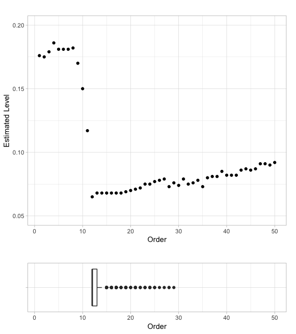 Figure 1
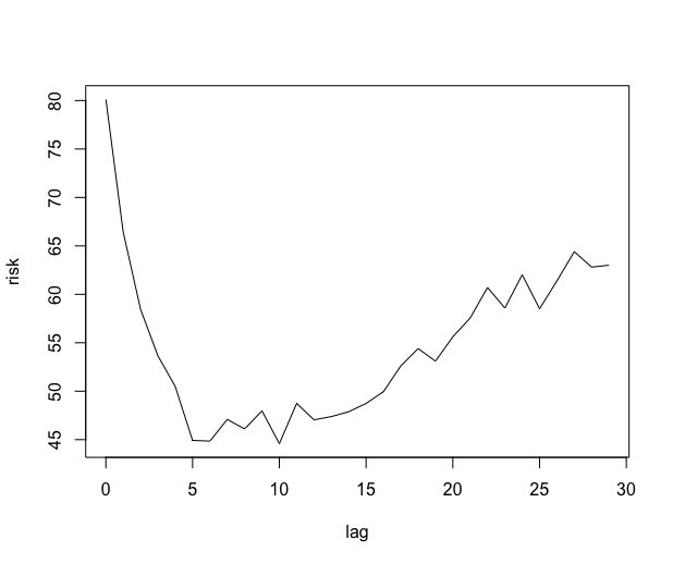 Figure 2
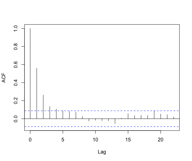 Figure 3
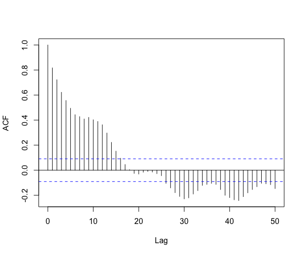 Figure 4
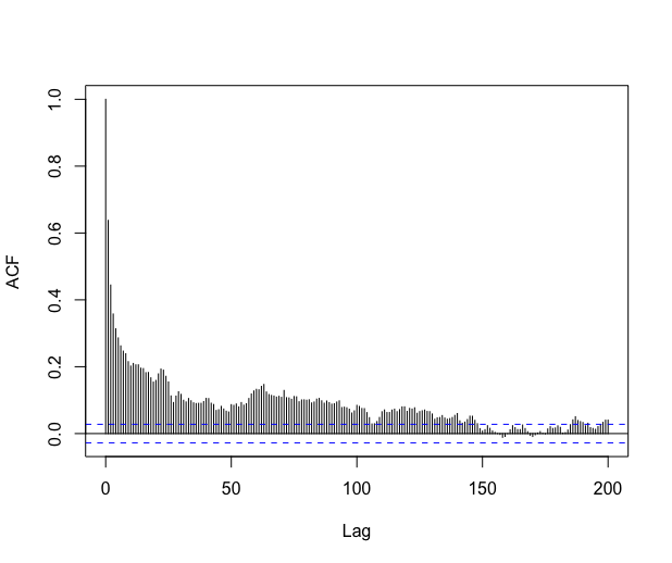 Figure 5
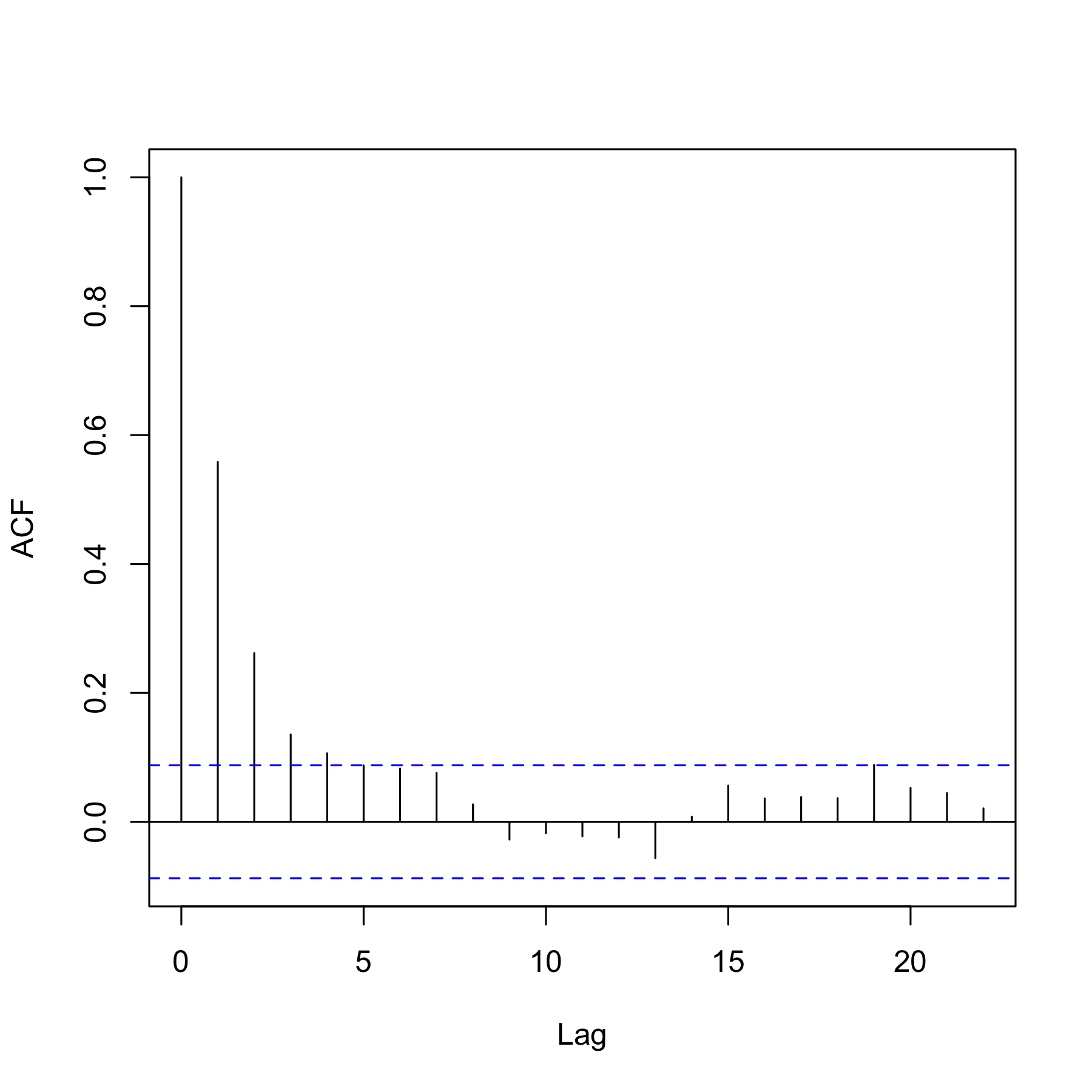 Figure 6
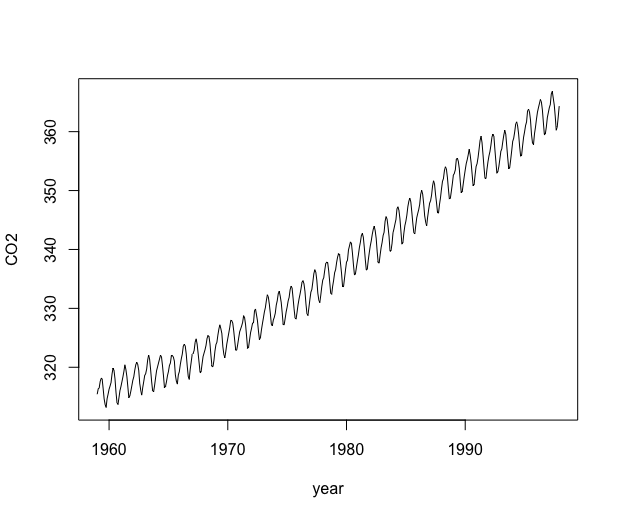 Figure 7
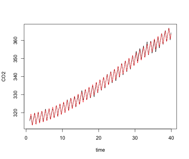 Figure 8
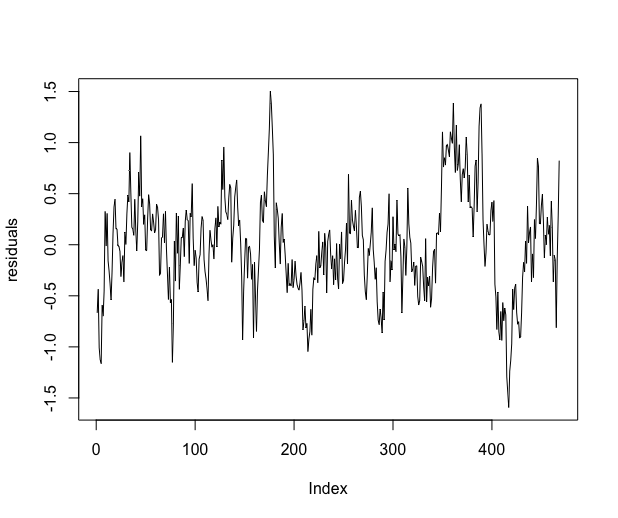 Figure 9
 Figure 10
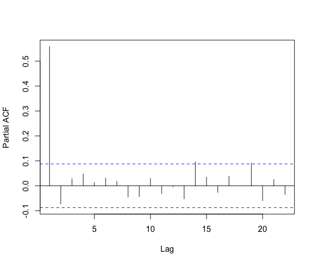 Figure 11
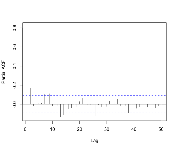 Figure 12
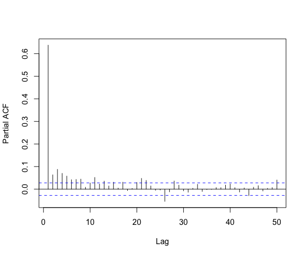 Figure 13
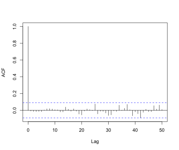 Figure 14
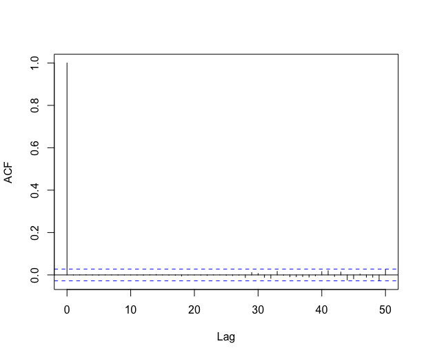 Figure 15
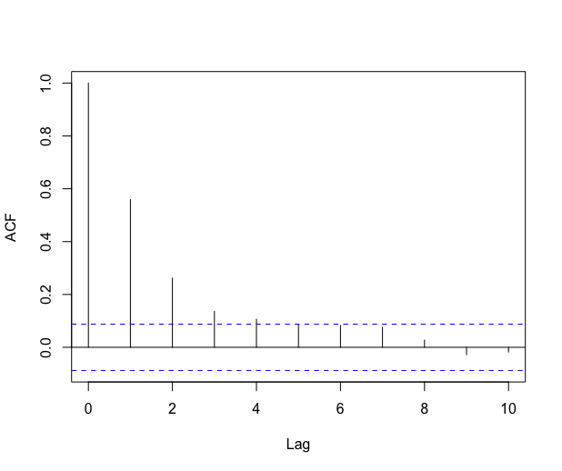 Figure 16
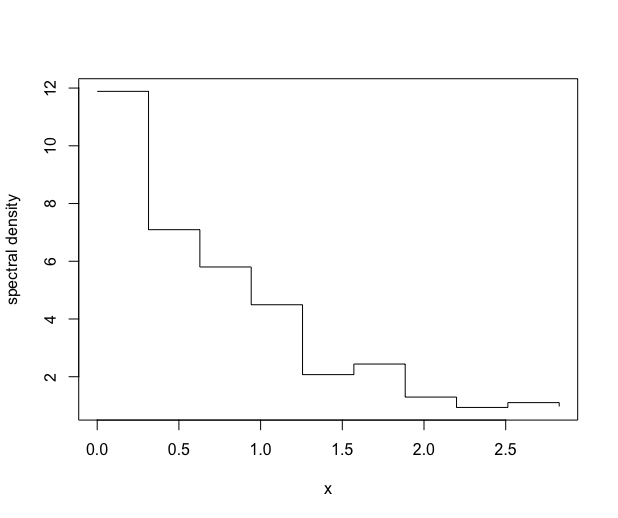 Figure 17
| \codemethod_cov_st= | plot |
|---|---|
| \codefitAR | ACF and PACF of the residual process |
| \codekernel | ACF of the residual process |
| \codekernel with \codemodel_selec = -1 | Graph of the estimated risk and of the estimated ’s |
| \codespectralproj | Estimated spectral density |
| \codeselect | ACF of the residuals up to the selected order |
| \codeefromovich | ACF of the residuals up to the selected order |
| \codehac | No plot available |
| \codekernel_fonc = | kernel definition |
|---|---|
| \coderectangular | |
| \codetriangle | |
| \codetrapeze |
| n | Fisher test | fitAR | spectralproj | efromovich | kernel | hac | |
|---|---|---|---|---|---|---|---|
| 200 | AR1 process | 0.465 | 0.097 | 0.14 | 0.135 | 0.149 | 0.108 |
| NonMixing | 0.298 | 0.082 | 0.103 | 0.096 | 0.125 | 0.064 | |
| Sysdyn process | 0.385 | 0.105 | 0.118 | 0.124 | 0.162 | 0.12 | |
| 1000 | AR1 process | 0.418 | 0.043 | 0.049 | 0.049 | 0.086 | 0.049 |
| NonMixing | 0.298 | 0.046 | 0.05 | 0.053 | 0.076 | 0.038 | |
| Sysdyn process | 0.393 | 0.073 | 0.077 | 0.079 | 0.074 | 0.078 | |
| 2000 | AR1 process | 0.454 | 0.071 | 0.078 | 0.075 | 0.067 | 0.071 |
| NonMixing | 0.313 | 0.051 | 0.053 | 0.057 | 0.067 | 0.047 | |
| Sysdyn process | 0.355 | 0.063 | 0.064 | 0.066 | 0.069 | 0.073 | |
| 5000 | AR1 process | 0.439 | 0.044 | 0.047 | 0.047 | 0.047 | 0.044 |
| NonMixing | 0.315 | 0.053 | 0.056 | 0.059 | 0.068 | 0.05 | |
| Sysdyn process | 0.381 | 0.058 | 0.061 | 0.057 | 0.064 | 0.071 |
| n | Fisher test | fitAR | spectralproj | efromovich | kernel | hac | |
|---|---|---|---|---|---|---|---|
| 200 | AR12 process | 0.436 | 0.178 | 0.203 | 0.223 | 0.234 | 0.169 |
| MA12 process | 0.228 | 0.113 | 0.113 | 0.116 | 0.15 | 0.222 | |
| 1000 | AR12 process | 0.468 | 0.068 | 0.183 | 0.181 | 0.124 | 0.179 |
| MA12 process | 0.209 | 0.064 | 0.066 | 0.069 | 0.063 | 0.18 | |
| 2000 | AR12 process | 0.507 | 0.071 | 0.196 | 0.153 | 0.104 | 0.192 |
| MA12 process | 0.237 | 0.064 | 0.064 | 0.058 | 0.068 | 0.173 | |
| 5000 | AR12 process | 0.47 | 0.062 | 0.183 | 0.1 | 0.091 | 0.171 |
| MA12 process | 0.242 | 0.044 | 0.048 | 0.043 | 0.057 | 0.147 |
| n | Fisher test | fitAR | spectralproj | efromovich | kernel | hac | |
|---|---|---|---|---|---|---|---|
| 150 | i.i.d. process | 0.053 | 0.068 | 0.078 | 0.061 | 0.124 | 0.063 |
| 300 | i.i.d. process | 0.052 | 0.051 | 0.06 | 0.05 | 0.095 | 0.052 |
| 500 | i.i.d. process | 0.047 | 0.049 | 0.053 | 0.049 | 0.082 | 0.056 |
Peer Reviews
No public reviews on file for this paper yet. If you reviewed it on a platform where reviews are public (OpenReview, ICLR, NeurIPS, ICML), you can paste yours below so the community can read it here.
Code & Models
Videos
No videos yet. Explain this paper in a talk, walkthrough, or lecture? Add one.
Taxonomy
TopicsAdvanced Statistical Methods and Models · Statistical Methods and Inference · Statistical Methods and Bayesian Inference
Linear regression with stationary errors : the \proglangR package \pkgslm
Emmanuel Caron
LMJL Ecole Centrale Nantes &Jérôme Dedecker
Université Paris Descartes &Bertrand Michel
LMJL Ecole Centrale Nantes
\Plainauthor
Emmanuel Caron, Jérôme Dedecker, Bertrand Michel
\PlaintitleLinear regression with stationary errors : the R package slm \ShorttitleLinear regression with stationary errors \AbstractThis paper introduces the \proglangR package \pkgslm which stands for Stationary Linear Models. The package contains a set of statistical procedures for linear regression in the general context where the error process is strictly stationary with short memory. We work in the setting of Hannan (1973), who proved the asymptotic normality of the (normalized) least squares estimators (LSE) under very mild conditions on the error process. We propose different ways to estimate the asymptotic covariance matrix of the LSE, and then to correct the type error rates of the usual tests on the parameters (as well as confidence intervals). The procedures are evaluated through different sets of simulations, and two examples of real datasets are studied. \KeywordsLinear model, Least Squares Estimators, Stationary processes, AutoRegressive processes, Spectral density, Hypothesis testing\PlainkeywordsLinear model, Least Squares Estimators, Stationary processes, AutoRegressive processes, Spectral density, Hypothesis testing \Address Emmanuel Caron, Bertrand Michel
Laboratoire de Mathématiques Jean Leray UMR 6629
Ecole Centrale Nantes
44300 Nantes, France
E-mail: ,
URL: http://ecaron.perso.math.cnrs.fr, http://bertrand.michel.perso.math.cnrs.fr
**
Jérôme Dedecker
Laboratoire MAP5 UMR 8145
Université Paris Descartes
75006 Paris, France
E-mail:
URL: http://w3.mi.parisdescartes.fr/~jdedecke/
**
1 Introduction
We consider the usual linear regression model
[TABLE]
where is the -dimensional vector of observations, is a (possibly random) design matrix, is a -dimensional vector of parameters, and is the error process (with zero mean and independent of ). The standard assumptions are that the ’s are independent and identically distributed (i.i.d.) with zero mean and finite variance.
In this paper, we propose to modify the standard statistical procedures (tests, confidence intervals, …) of the linear model in the more general context where the ’s are obtained from a strictly stationary process with short memory. To be more precise, let denote the usual least squares estimator of . Our approach is based on two papers: the paper by Hannan (1973) who proved the asymptotic normality of the least squares estimator ( being the usual normalization) under very mild conditions on the design and on the error process; and a recent paper by Caron (2019) who showed that, under Hannan’s conditions, the asymptotic covariance matrix of can be consistently estimated.
Let us emphasize that Hannan’s conditions on the error process are very mild and are satisfied for most of short-memory processes (see the discussion in Section of Caron and Dede (2018)). Putting together the two above results, we can develop a general methodology for tests and confidence regions on the parameter , which should be valid for most of short-memory processes. This is of course directly useful for time-series regression (we shall present in Section 5 an application to the "Mona Loa" \proglangR data-set on CO2 concentration), but also in the more general context where the residuals of the linear model seem to be strongly correlated. More precisely, when checking the residuals of the linear model, if the autocorrelation function of the residuals shows significant correlations, and if the residuals can be suitably modeled by an ARMA process, then our methodology is likely to apply. We shall give an example of such a situation in Section 5 (Shangai pollution data-set).
Hence, the tools presented in the present paper can be seen from two different points of view:
as appropriate tools for time series regression with short memory error process.
- -
as a way to robustify the usual statistical procedures when the residuals are correlated.
Let us now describe the organisation of the paper. In Section 2, we recall the mathematical background, the consistent estimator of the asymptotic covariance matrix introduced in Caron (2019) and the modified -statistics and -square statistics for testing hypothesis on the parameter . In Section 3 we present the \pkgslm package, and the different ways to estimate the asymptotic covariance matrix: by fitting an autoregressive process on the residuals (default procedure), by means of the kernel estimator described in Caron (2019) (theoretically valid) with a bootstrap method to choose the bandwidth (Wu and Pourahmadi (2009)), by using alternative choices of the bandwidth for the rectangular kernel (Efromovich (1998)) and the quadratic spectral kernel (Andrews (1991)), by means of an adaptative estimator of the spectral density via Histograms (Comte (2001)). In Section 4, we estimate the level of a -square test for a linear model with random design, with different kinds of error processes and for different estimation procedures. In Section 5, we present two different data sets "CO2 concentration", "Shangai pollution", and we compare the summary output of \codeslm with the usual summary output of \codelm.
2 Linear regression with stationary errors
2.1 Asymptotic results for the kernel estimator
We start this section by giving a short presentation of linear regression with stationary errors, more details can be found for instance in Caron (2019). Let be the usual least squares estimator for the unknown vector . The aim is to provide hypothesis tests and confidence regions for in the non i.i.d. context.
Let be the autocovariance function of the error process : for any integers and , let . We also introduce the covariance matrix
[TABLE]
Hannan (1973) has shown a Central Limit Theorem for when the error process is strictly stationary, under very mild conditions on the design and the error process. Let us notice that the design can be random or deterministic. We introduce the normalization matrix which is a diagonal matrix with diagonal term for in , where is the th column of . Roughly speaking, Hannan’s result says in particular that, given the design , the vector converges in distribution to a centered Gaussian distribution with covariance matrix . As usual, in practice the covariance matrix is unknown and it has to be estimated. Hannan also showed the convergence of second order moment:111The transpose of a matrix is denoted by .
[TABLE]
where
[TABLE]
In this paper we propose a general plug-in approach: for some given estimator of , we introduce the plug-in estimator
[TABLE]
and we use to standardize the usual statistics considered for the study of linear regression.
Let us illustrate this plug-in approach with a kernel estimator which has been proposed in Caron (2019). For some and a bandwidth , the kernel estimator is defined by
[TABLE]
where the residual based empirical covariance coefficients are defined for by
[TABLE]
For a well-chosen kernel and under mild assumptions on the design and the error process, it has been proved in Caron (2019) that
[TABLE]
for the plug-in estimator , for some suitable sequence of bandwidths .
More generally, in this paper we say that an estimator of is consistent for estimating the covariance matrix if is positive definite and if it converges in probability to . Note that such a property requires assumptions on the design, see Caron (2019). If is consistent for estimating the covariance matrix , then converges in distribution to a standard Gaussian vector.
To conclude this section, let us make some additional remarks. The interest of Caron’s recent paper is that the consistency of the estimator is proved under Hannan’s condition on the error process, which is known to be optimal with respect to the convergence in distribution (see for instance Dedecker (2015)), and which allows to deal with most short memory processes. But the natural estimator of the covariance matrix of based on has been studied by many other authors in various contexts. For instance, let us mention the important line of research initiated by Newey and West (1987, 1994), and the related papers by Andrews (1991); Andrews and Monahan (1992) among others. In the paper by Andrews (1991), the consistency of the estimator based on is proved under general conditions on the fourth order cumulants of the error process, and a data driven choice of the bandwidth is proposed. Note that these authors also considered the case of heteroskedastic processes. Most of these procedures, known as HAC (Heteroskedasticity and Autocorrelation Consistent) procedures, are implemented in the package \pkgsandwich by Zeileis, Lumley, Berger and Graham222See the CRAN website: https://cran.r-project.org/web/packages/sandwich/index.html., and presented in great detail in the paper by Zeileis (2004). We shall use an argument of the \pkgsandwich package, based on the data driven procedure described by Andrews (1991) at the end of Section 3.2 (see also Section 4 for a comparison with other methods).
2.2 Tests and confidence regions
We now present tests and confidence regions for arbitrary estimators . The complete justifications are available for kernel estimators, see Caron (2019).
Z-Statistics.
We introduce the following univariate statistics:
[TABLE]
where . If is consistent for estimating the covariance matrix and if , the distribution of converges to a standard normal distribution when tends to infinity. We directly derive an asymptotic hypothesis test for testing against as well as an asymptotic confidence interval for .
Chi-square statistics.
Let be a matrix with . Under Hannan (1973)’s conditions, converges in distribution to a centered Gaussian distribution with covariance matrix . If is consistent for estimating the covariance matrix , then converges in probability to . The matrix being symmetric positive definite, this yields
[TABLE]
This last result provides asymptotical confidence regions for the vector . It also provides an asymptotic test for testing the hypothesis : against : . Indeed, under the -hypothesis, the distribution of converges to a -distribution.
The test can be used to simplify a linear model by testing that several linear combinations between the parameters are zero, as we usually do for Anova and regression models. In particular, with , the test corresponds to the test of overall significance.
3 Introduction to linear regression with the slm package
Using the \pkgslm package is very intuitive because the arguments and the outputs of \codeslm are similar to those of the standard functions \codelm, \codeglm, etc. The output of the main function \codeslm is an object of class \codeslm , a specific class that has been defined for linear regression with stationary processes. The \codeslm class has methods \codeplot, \codesummary, \codeconfint and \codepredict. Moreover, the class \codeslm inherits from the \codelm class and thus provides the output of the classical \codelm function.
R> library(slm)
The statistical tools available in \codeslm strongly depend on the choice of the covariance plug-in estimator we use for estimating . All the estimators proposed in \codeslm are residual-based estimators, but they rely on different approaches. In this section, we present the main functionality of \codeslm together with the different covariance plug-in estimators.
For illustrating the package, we simulate synthetic data according to the linear model:
[TABLE]
where is a gaussian autoregressive process of order , and is the Nonmixing process described in Section 4.1. We use the functions \codegenerative_model and \codegenerative_process respectively to simulate observations according to this regression design and with this specific stationary process. More details on the designs and the processes available with
\codegenerative_model and \codegenerative_process are given in Section 4.1.
R> n = 500R> eps = generative_process(n,"Nonmixing")R> design = generative_model(n,"mod2")R> design_sim = cbind(rep(1,n), as.matrix(design))R> beta_vec = c(2,0.001,0.5)R> Y = design_sim %*% beta_vec + eps
3.1 Linear regression via AR fitting on the residuals
A large class of stationary processes with continuous spectral density can be well approximated by AR processes, see for instance Corollary 4.4.2 in Brockwell and Davis (1991). The covariance structure of an AR process having a closed form, it is thus easy to derive an approximation of by fitting an AR process on the residual process.
The AR-based method for estimating is the default version of \codeslm. This method proceeds in four main steps:
Fit an autoregressive process on the residual process ; 2. 2.
Compute the theoretical covariances of the fitted AR process ; 3. 3.
Plug the covariances in the Toeplitz matrix ; 4. 4.
Compute .
The \codeslm function fits a linear regression of the vector on the design and then fits an AR process on the residual process using the \codear function from the \pkgstats package. The output of the \codeslm function is an object of class \codeslm. The order of the AR process is set in the argument \codemodel_selec:
R> regslm = slm(Y ~ X1+X2, data = design, method_cov_st = "fitAR",+ model_selec = 3) The estimated covariance is recorded as a vector in the attribute \codecov_st of \coderegslm, which is an object of class \codeslm. The estimated covariance matrix can be computed by taking the Toeplitz matrix of \codecov_st, using the \codetoeplitz function.
Summary method
As for \codelm objects, a summary of a \codeslm object is given by
R> summary(regslm)
Call:"slm(formula = myformula, data = data, x = x, y = y)"Residuals: Min 1Q Median 3Q Max-13.9086 -3.4586 0.1646 3.5025 13.7488Coefficients: Estimate Std. Error z value Pr(>|z|)(Intercept) 2.936183 0.855214 3.433 0.000596 X1 0.084387 0.082371 1.024 0.305613X2 0.492590 0.002738 179.938 < 2e-16 ---Signif. codes: 0 ’’ 0.001 ’’ 0.01 ’’ 0.05 ’.’ 0.1 ’ ’ 1Residual standard error: 4.907Multiple R-squared: 0.9953chi2-statistic: 3.278e+04 on 2 DF, p-value: < 2.2e-16 The coefficient table output by the summary provides the estimators of the ’s, which are exactly the classical least squares estimators. The \codez value column provides the values of the statistics defined by (4). The \codeStd.Error column gives an estimation of the standard errors of the ’s, which are taken equal to . As with the \codelm function, the p-value column is the p-value for testing against . In this example, the small p-value for the second feature is consistent with the value chosen for \codebeta_vec at the beginning of the section. The \codechi2-statistic at the end of the summary is the statistic for testing the significance of the model (see the end of Section 2.2) For this example, the p-value is very small, indeed the variable has a significant effect on .
Plot argument and plot method
The \codeslm function has a \codeplot argument: with \codeplot = TRUE, the function plots a figure which depends on the method chosen for estimating the covariance matrix . Table 1 summarizes the plots for each method given in the argument \codemethod_cov_st. With the AR fitting method, the argument \codeplot = TRUE outputs the ACF and the PACF of the residual process. The ACF and PACF are computed with the functions \codeacf and \codepacf of the \pkgstats package. As usual, the ACF and PACF graphs should help the user to choose an appropriate order for the AR process.
R> regslm = slm(Y ~ X1 + X2, data = design, method_cov_st = "fitAR",+ model_selec = 2, plot = TRUE) The plot output by the \codeslm function for this example is given in Figure 1.
Since the \codeslm class inherits from the \codelm class, the former class comes with a \codeplot method which is the same as for the \codelm class, namely the diagnostic analysis of the linear regression. The graphics are displayed using the command
R> plot(regslm)
Confidence intervals for the coefficients
The \codeconfint function computes the confidence intervals for the coefficients estimated by \codeslm. These intervals are computed according to the distribution of the statistics defined in (4).
R> confint(regslm, level = 0.90)
5 % 95 %(Intercept) 1.56396552 4.3083996X1 -0.05048587 0.2192597X2 0.48821351 0.4969666
AR order selection
The order of the AR process can be chosen at hand by setting \codemodel_selec = p, or automatically with the AIC criterion by setting \codemodel_selec = -1.
R> regslm = slm(Y ~ X1 + X2, data = design, method_cov_st = "fitAR",+ model_selec = -1) The order of the fitted AR process is recorded in the \codemodel_selec attribute of \coderegslm:
R> regslm@model_selec
[1] 2 Here, the AIC criterion suggests to fit an AR(2) process on the residuals.
3.2 Linear regression via kernel estimation of the error covariance
The second method for estimating the covariance matrix is the kernel estimation method (1) studied in Caron (2019). In short, this method estimates via a smooth approximation of the covariance matrix of the residuals. This estimation of corresponds to the so-called tapered covariance matrix estimator in the literature, see for instance Xiao and Wu (2012), or also to the "lag-window estimator" defined in Brockwell and Davis (1991), page . It applies in particular for non negative symmetric kernels with compact support, with an integrable Fourier transform and such that . Table 2 gives the list of the available kernels in the package \pkgslm.
It is also possible for the user to define his own kernel and to use it in the argument \codekernel_fonc of the \codeslm function. Below we use the triangle kernel which assures that the covariance matrix is positive definite. The support of the kernel in Equation (1) being compact, only the terms for small enough lag are kept and weighted by the kernel in the expression of . Rather than setting the bandwidth , we select the number of ’s that should be kept (the lag) with the argument \codemodel_selec in the \codeslm function. Then the bandwidth is calibrated accordingly, that is equal to .
R> regslm = slm(Y ~ X1 + X2, data = design, method_cov_st = "kernel",+ model_selec = 5, kernel_fonc = triangle, plot = TRUE) The plot output by the \codeslm function is given in Figure 2.
Order selection via bootstrap
The order parameter can be chosen at hand as before or automatically by setting \codemodel_selec = -1. The automatic order selection is based on the bootstrap procedure proposed by Wu and Pourahmadi (2009) for banded covariance matrix estimation. The \codeblock_size argument sets the size of bootstrap blocks and the \codeblock_n argument sets the number of blocks. The final order is chosen by taking the order which has the minimal risk. Figure 3 gives the plots of the estimated risk for the estimation of (left) and the final estimated ACF (right).
R> regslm = slm(Y ~ X1 + X2, data = design, method_cov_st ="kernel",+ model_selec = -1, kernel_fonc = triangle, model_max = 30,+ block_size = 100, block_n = 100, plot = TRUE)
The selected order is recorded in the \codemodel_selec attribute of the \codeslm object output by the \codeslm function:
R> regslm@model_selec
[1] 10
3.2.1 Order selection by Efromovich’s method (rectangular kernel)
An alternative method for choosing the bandwidth in the case of the rectangular kernel has been proposed in Efromovich (1998). For a large class of stationary processes with exponentially decaying autocovariance function (mainly the ARMA processes), Efromovich proved that the rectangular kernel is asymptotically minimax, and he proposed the following estimator:
[TABLE]
with the lag
[TABLE]
where is a regularity index of the autocovariance index. In practice this parameter is unknown and is estimated thanks to the algorithm proposed in the section of Efromovich (1998). As for the other methods, we use the residual based empirical covariances to compute .
R> regslm = slm(Y ~ X1 + X2, data = design, method_cov_st = "efromovich",+ model_selec = -1)
3.2.2 Order Selection by Andrews’s method
Another method for choosing the bandwidth has been proposed by Andrews (1991) (see the last paragraph of Section 2.1) and implemented in the package \pkgsandwich by Zeileis, Lumley, Berger and Graham (see the paper by Zeileis (2004)). For the \pkgslm package, the automatic choice of the bandwidth proposed by Andrews can be obtained as follows
R> regslm = slm(Y ~ X1 + X2, data = design, method_cov_st = "hac") The procedure is based on the function \codekernHAC in the \pkgsandwich package. This function computes directly the covariance matrix estimator of , which will be recorded in the slot \codeCov_ST of the \codeslm function.
Here, we take the quadratic spectral kernel
[TABLE]
as suggested by Andrews (see Section in Andrews (1991), or Section in Zeileis (2004)), but other kernels could be used, such as Bartlett, Parzen, Tukey-Hamming, among others (see Zeileis (2004)).
Positive definite projection
Depending of the method used, the matrix may not always be positive definite. It is the case of the kernel method with rectangular or trapeze kernel. To overcome this problem, we make the projection of into the cone of positive definite matrices by applying a hard thresholding on the spectrum of this matrix: we replace all eigenvalues lower or equal to zero with the smallest positive eigenvalue of .
Note that this projection is useless for the triangle or quadratic spectral kernels because their Fourier transform is non-negative (leading to a positive definite matrix ). Of course, it is also useless for the \codefitAR and \codespectralproj methods.
3.3 Linear regression via projection spectral estimation
The projection method relies on the ideas of Comte (2001), where an adaptive nonparametric method has been proposed for estimating the spectral density of a stationary Gaussian process.
We use the residual process as a proxy for the error process and we compute the projection coefficients with the residual-based empirical covariance coefficients , see Equation (2).
For some , the estimator of the spectral density of the error process that we use is defined by computing the projection estimators for the residual process, on the basis of histogram functions
[TABLE]
The estimator is defined by
[TABLE]
where the projection coefficients are
[TABLE]
The Fourier coefficients of the spectral density are equal to the covariance coefficients. Thus, for it yields
[TABLE]
and for :
[TABLE]
This method can be proceeded in the \codeslm function by setting \codemethod_cov_st =
\code"spectralproj":
R> regslm = slm(Y ~ X1 + X2, data = design, method_cov_st = "spectralproj",+ model_selec = 10, plot = TRUE) The graph of the estimated spectral density can be plotted by setting \codeplot = TRUE in the \codeslm function, see Figure 4.
Model selection
The Gaussian model selection method proposed in Comte (2001) follows the ideas of Birgé and Massart, see for instance Massart (2007). It consists in minimizing the penalized criterion, see Section 5 in Comte (2001):
[TABLE]
where is a multiplicative constant that in practice can be calibrated using the slope heuristic method, see Birgé and Massart (2007); Baudry et al. (2012) and the \proglangR package \pkgcapushe.
R> regslm = slm(Y ~ X1 + X2, data = design, method_cov_st = "spectralproj",+ model_selec = -1, model_max = 50, plot = TRUE) The selected dimension is recorded in the \codemodel_selec attribute of the \codeslm object output by the \codeslm function:
R> regslm@model_selec
[1] 8 The slope heuristic algorithm here selects an Histogram on a regular partition of size over the interval to estimate the spectral density.
3.4 Linear regression via masked covariance estimation
This method is a full-manual method for estimating the covariance matrix by only selecting covariance terms from the residual covariances defined by (2). Let be a set of positive integers, then we consider
[TABLE]
and then we define the estimated covariance marix by taking the Toeplitz matrix of the vector . This estimator is a particular example of masked sample covariance estimator, as introduced by Chen et al. (2012), see also Levina and Vershynin (2012). Finally we derive from an estimator for .
The next instruction selects the coefficients 0, 1, 2 and 4 from the residual covariance terms:
R> regslm = slm(Y ~ X1 + X2, data = design, method_cov_st = "select",+ model_selec = c(1,2,4)) The positive lags of the selected covariances are recordered in the \codemodel_selec argument. Let us notice that the variance is automatically selected.
As for the kernel method, the resulting covariance matrix may not be positive definite. If it is the case, the positive definite projection method, described at the end of the section 3.2, is used.
3.5 Linear regression via manual plugged covariance matrix
This last method is a direct plug-in method. The user proposes his own vector estimator of and then the Toeplitz matrix of the vector is used for estimating with .
R> v = rep(0,n)R> v[1:10] = acf(epsilon, type = "covariance", lag.max = 9)$acfR> regslm = slm(Y ~ X1 + X2, data = design, cov_st = v)
The user can also propose his own covariance matrix for estimating .
R> v = rep(0,n)R> v[1:10] = acf(epsilon, type = "covariance", lag.max = 9)$acfR> V = toeplitz(v)R> regslm = slm(Y ~ X1 + X2, data = design, Cov_ST = V)
Let us notice that the user must verify that the resulting covariance matrix is positive definite. The positive definite projection algorithm is not used with this method.
4 Numerical experiments and method comparisons
This section summarizes an extensive study which has been carried out to compare the performances of the different approaches presented before in the context of linear model with short range dependent stationary errors.
4.1 Description of the generative models
We first present the five generative models for the errors that we consider in the paper. We choose different kinds of processes to reflect the diversity of short-memory processes.
- •
AR1 process. The AR1 process is a gaussian AR(1) process defined by:
[TABLE]
where is a standard gaussian distribution .
- •
AR12 process. The AR12 process is a seasonal AR(12) process defined by:
[TABLE]
where is a standard gaussian distribution . When studying monthly data-sets, one usually observes a seasonality of order . For example, when looking at climate data (such as the "CO2 concentration" dataset of Section 5), the data are often collected per month, and the same phenomenon tends to repeat every year. Even if the design integrates the deterministic part of the seasonality, a correlation of order remains usually present in the residual process.
- •
MA12 process. The MA12 is also a seasonal process defined by:
[TABLE]
where the ’s are i.i.d. random variables following Student’s distribution with degrees of freedom.
- •
Nonmixing process. The three processes described above are basic ARMA processes, whose innovations have absolutely continuous distributions; in particular, they are strongly mixing in the sense of Rosenblatt (1956), with a geometric decay of the mixing coefficients (in fact the MA12 process is even -dependent, which means that the mixing coefficient if ). Let us now describe a more complicated process: let satisfying the AR(1) equation
[TABLE]
where is uniformly distributed over and the ’s are i.i.d. random variables with distribution , independent of . The process is a strictly stationary Markov chain, but it is not -mixing in the sense of Rosenblatt (see Bradley (1986)). Let now be the inverse of the cumulative distribution function of a centered Gaussian distribution with variance (for the simulations below, we choose ). The Nonmixing process is then defined by
[TABLE]
The sequence is also a stationary Markov chain (as an invertible function of a stationary Markov chain). By construction, is -distributed, but the sequence is not a Gaussian process (otherwise it would be mixing in the sense of Rosenblatt). Although it is not obvious, one can prove that the process satisfies Hannan’s condition (see Caron (2019), Section ).
- •
Sysdyn process. The four processes described above have the property of "geometric decay of correlations", which means that the ’s tend to [math] at an exponential rate. However, as already pointed out in the introduction, Hannan’s condition is valid for most of short memory processes, even for processes with slow decay of correlations (provided that the ’s are summable). Hence, our last example will be a non-mixing process (in the sense of Rosenblatt), with an arithmetic decay of the correlations.
For , the intermittent map introduced in Liverani et al. (1999) is defined by
[TABLE]
It follows from Liverani et al. (1999) that there exists a unique -invariant probability measure . The Sysdyn process is then defined by
[TABLE]
From Liverani et al. (1999), we know that, on the probability space , the autocorrelations of the stationary process are exactly of order . Hence is a short memory process provided . Moreover, it has been proved in Section of Caron and Dede (2018) that satisfies Hannan’s condition in the whole short-memory range, that is for . For the simulations below, we took , which give autocorrelations of order .
The linear regression models simulated in the experiments all have the following form:
[TABLE]
where is a gaussian autoregressive process of order and is one of the stationary processes defined above. For the simulations, is always equal to . All the error processes presented above can be simulated with the \pkgslm package with the \codegenerative_process function. The design can be simulated with the \codegenerative_model function.
4.2 Automatic calibration of the tests
It is of course of first importance to provide hypothesis tests with correct significance levels or at least with correct asymptotical significance levels, which is possible if the estimator of the covariance matrix is consistent for estimating . For instance, the results of Caron (2019) show that it is possible to construct statistical tests with correct asymptotical significance levels. However in practice such asymptotical results are not sufficient since they do not indicate how to tune the bandwidth on a given dataset. This situation makes the practice of linear regression with dependent errors really more difficult than linear regression with i.i.d. errors. This problem happens for several methods given before : order choice for the \codefitAR method, bandwidth choice for the \codekernel method, dimension selection for the \codespectralproj method.
It is a tricky issue to design a data driven procedure for choosing test parameters in order to have to correct Type I Error. Note that unlike with supervised problems and density estimation, it is not possible to calibrate hypothesis tests in practice using cross validation approaches. We thus propose to calibrate the tests using well founded statistical procedures for risk minimization : AIC criterion for the \codefitAR method, bootstrap procedures for the \codekernel method and slope heuristics for the \codespectralproj method. These procedures are implemented in the \codeslm function with the \codemodel_selec = -1 argument, as detailed in the previous section.
Let us first illustrate the calibration problem with the AR12 process. For simulations, we generate an error process of size under the null hypothesis: . Then we use the \codefitAR method of the \codeslm function with orders between and and we perform the model significance test. The procedure is repeated times and we estimate the true level of the test by taking the average of the estimated levels on the simulations for each order. The results are given on Figure 5 for . A boxplot is also displayed to visualize the distribution of the order selected by the automatic criterion (AIC).
4.3 Non-Seasonal errors
We first study the case of non-Seasonal error processes. We simulate a -error process according to the AR1, the Nonmixing or the Sysdyn processes. We simulate realizations of the linear regression model (5) under the null hypothesis: . We use the automatic selection procedures for each method (\codemodel_selec = -1). The simulations are repeated times in order to estimate the true level of the model significance for each test procedure. We simulate either small samples () or larger samples (). The results of this experiments are summarized in Table 3.
For large enough (), all methods work well and the estimated level is around . However, for small samples (), we observe that the \codefitAR and the \codehac methods show better performances than the others. The \codekernel method is slightly less effective. With this method, we must choose the size of the bootstrap blocks as well as the number of blocks and the test results are really sensitive to these parameters. In these simulations, we have chosen blocks with a size of . The results are expected to improve with a larger number of blocks.
Let us notice that for all methods and for all sample sizes, the estimated level is much better than if no correction is made (usual Fisher tests).
4.4 Seasonal errors
We now study the case of linear regression with seasonal errors. The experiment is exactly the same as before, except that we simulate AR12 or MA12 processes. The results of these experiments are summarized in Table 4.
We directly see that the case of seasonal processes is more complicated than for the non-seasonal processes especially for the AR12 process. For small samples size, the estimated level is between and , which is clearly too large. It is however much better than the estimated level of the usual Fisher test, which is around . The \codefitAR method is the best method here for the AR12 process, because for , the estimated level is between and . For \codeefromovich and \codekernel methods, a level less than is reached but for large samples only. The \codespectralproj and \codehac methods do not seem to work well for the AR12 process, although they remain much better than the usual Fisher tests (around of rejection instead of ).
The case of the MA12 process seems easier to deal with. For large enough (), the estimated level is between and whatever the method, except for \codehac (around for ). It is less effective for small sample size () with an estimated level around for \codefitAR, \codespectralproj and \codeefromovich methods.
4.5 I.I.D. errors
To be complete, we consider in this subsection the case where the ’s are i.i.d., to see how the five automatic methods perform in that case.
We simulate i.i.d. centered random variables according to the formula:
[TABLE]
where follows a student distribution with degrees of freedom. Note that the distribution of the ’s is not symmetric and has no exponential moments.
Except for the kernel method, the estimated levels are close to for large enough (). It is slightly worse for small samples but it remains quite good for the methods \codefitAR, \codeefromovich and \codehac.
As a general conclusion of Section , we see that the \codefitAR method performs quite well in a wide variety of situations, and should therefore be used as soon as the user suspects that the error process can be modeled by a stationary short-memory process.
5 Application to real data
5.1 Data CO2
Let us introduce the first dataset that we want to study. It concerns the well-known dataset "co2", available in the package \pkgdatasets of \proglangR:
R> data("co2") This dataset is provided by the observatory of Mona Loa (Hawaii). It contains average monthly measurements of CO2 (parts per million: ppmv) in the atmosphere of the Hawaiian coast. Surveys were produced monthly between and , giving a total of measurements. The graph of the data is displayed in Figure 6. More information on this dataset is available in the \proglangR documentation.
We model the CO2 measurements with a time series. Typically, a time series can be decomposed into three parts: a trend and a seasonality , which are deterministic components, and the errors , which constitute the random part of the model. The trend represents the overall behavior of the series and seasonality its periodic behavior. Formally, we have:
[TABLE]
where represents the CO2 rate at time , with the usual constraints and . The two deterministic components can be grouped into a matrix and the model can be rewritten into a linear regression model:
[TABLE]
For this example, we fit a -degree polynomial for the trend and a trigonometric polynomial with well-chosen frequencies for the seasonality. Here the time represents a month and goes from to by step of length . Let us perform a linear regression to fit the trend and the seasonality on the CO2 time series, using the \codelm function:
R> y = as.vector(co2)R> t = as.vector(time(co2)) - 1958R> regtrigo = lm(y ~ t + I(t^2) + I(t^3) + sin(2pit) + cos(2pit)+ + sin(4pit) + cos(4pit) + sin(6pit) + cos(6pit)+ + sin(8pit) + cos(8pit)) We obtain the following output:
R> summary.lm(regtrigo)
Call:lm(formula = y ~ t + I(t^2) + I(t^3) + sin(2 * pi * t) + cos(2 * pi * t) + sin(4 * pi * t) + cos(4 * pi * t) + sin(6 * pi * t) + cos(6 * pi * t) + sin(8 * pi * t) + cos(8 * pi * t))Residuals: Min 1Q Median 3Q Max-1.54750 -0.32688 0.00233 0.28100 1.50295Coefficients: Estimate Std. Error t value Pr(>|t|)(Intercept) 3.157e+02 1.118e-01 2823.332 < 2e-16 ***t 3.194e-01 2.306e-02 13.847 < 2e-16 ***I(t^2) 4.077e-02 1.293e-03 31.523 < 2e-16 ***I(t^3) -4.562e-04 2.080e-05 -21.930 < 2e-16 ***sin(2 * pi * t) 2.751e+00 3.298e-02 83.426 < 2e-16 ***cos(2 * pi * t) -3.960e-01 3.296e-02 -12.015 < 2e-16 ***sin(4 * pi * t) -6.743e-01 3.296e-02 -20.459 < 2e-16 **cos(4 * pi * t) 3.785e-01 3.296e-02 11.484 < 2e-16 sin(6 * pi * t) -1.042e-01 3.296e-02 -3.161 0.00168 **cos(6 * pi * t) -4.389e-02 3.296e-02 -1.332 0.18362sin(8 * pi * t) 8.733e-02 3.296e-02 2.650 0.00833 cos(8 * pi * t) 2.559e-03 3.296e-02 0.078 0.93814---Signif. codes: 0 ’’ 0.001 ’’ 0.01 ’’ 0.05 ’.’ 0.1 ’ ’ 1Residual standard error: 0.5041 on 456 degrees of freedomMultiple R-squared: 0.9989,Adjusted R-squared: 0.9989F-statistic: 3.738e+04 on 11 and 456 DF, p-value: < 2.2e-16 We see in the summary that two variables have no significant effect on the CO2 rate. Next, we perform a backward selection method with a p-value threshold equal to . This selects the following model:
R> regtrigo = lm(y ~ t + I(t^2) + I(t^3) + sin(2pit) + cos(2pit)+ + sin(4pit) + cos(4pit) + sin(6pit) + sin(8pit)) with the corresponding summary
R> summary.lm(regtrigo)
Call:lm(formula = y ~ t + I(t^2) + I(t^3) + sin(2 * pi * t) + cos(2 * pi * t) + sin(4 * pi * t) + cos(4 * pi * t) + sin(6 * pi * t) + sin(8 * pi * t))Residuals: Min 1Q Median 3Q Max-1.59287 -0.32364 0.00226 0.29884 1.50154Coefficients: Estimate Std. Error t value Pr(>|t|)(Intercept) 3.157e+02 1.118e-01 2824.174 < 2e-16 ***t 3.196e-01 2.306e-02 13.861 < 2e-16 ***I(t^2) 4.075e-02 1.293e-03 31.522 < 2e-16 ***I(t^3) -4.560e-04 2.080e-05 -21.927 < 2e-16 ***sin(2 * pi * t) 2.751e+00 3.297e-02 83.446 < 2e-16 ***cos(2 * pi * t) -3.960e-01 3.295e-02 -12.018 < 2e-16 ***sin(4 * pi * t) -6.743e-01 3.295e-02 -20.464 < 2e-16 **cos(4 * pi * t) 3.785e-01 3.295e-02 11.487 < 2e-16 sin(6 * pi * t) -1.042e-01 3.295e-02 -3.162 0.00167 **sin(8 * pi * t) 8.734e-02 3.295e-02 2.651 0.00831 ---Signif. codes: 0 ’’ 0.001 ’’ 0.01 ’’ 0.05 ’.’ 0.1 ’ ’ 1Residual standard error: 0.504 on 458 degrees of freedomMultiple R-squared: 0.9989,Adjusted R-squared: 0.9989F-statistic: 4.57e+04 on 9 and 458 DF, p-value: < 2.2e-16
The sum of the estimated trend and estimated tendency is displayed on the left plot of Figure 7, and the residuals are displayed on the right plot.
The \codelm procedure assumes that the errors are independent, but if we look at the autocorrelation function of the residual process we clearly observe that the residuals are strongly correlated, see Figure 8. Consequently, the \codelm procedure may be unreliable in this context.
The autocorrelation function of the residuals decreases rather fast. Looking at the partial autocorrelation function, it seems reasonable to fit an AR process on the residuals. The automatic \codefitAR method selects an AR of order and the residuals look like a white noise, see Figure 9.
We now use the \codeslm function with the \codefitAR method with the following complete model
R> regtrigo = slm(y ~ t + I(t^2) + I(t^3) + sin(2pit) + cos(2pit)+ + sin(4pit) + cos(4pit) + sin(6pit) + cos(6pit)+ + sin(8pit) + cos(8pit), method_cov_st = "fitAR",+ model_selec = -1) Let us display the summary of the procedure:
R> summary(regtrigo)
Call:"slm(formula = myformula, data = data, x = x, y = y)"Residuals: Min 1Q Median 3Q Max-1.54750 -0.32688 0.00233 0.28100 1.50295Coefficients: Estimate Std. Error z value Pr(>|z|)(Intercept) 3.157e+02 3.968e-01 795.646 < 2e-16 ***t 3.194e-01 8.222e-02 3.884 0.000103 ***I(t^2) 4.077e-02 4.619e-03 8.825 < 2e-16 ***I(t^3) -4.562e-04 7.430e-05 -6.140 8.23e-10 ***sin(2 * pi * t) 2.751e+00 4.739e-02 58.054 < 2e-16 ***cos(2 * pi * t) -3.960e-01 4.716e-02 -8.396 < 2e-16 ***sin(4 * pi * t) -6.743e-01 2.051e-02 -32.875 < 2e-16 ***cos(4 * pi * t) 3.785e-01 2.041e-02 18.548 < 2e-16 ***sin(6 * pi * t) -1.042e-01 1.359e-02 -7.663 1.82e-14 **cos(6 * pi * t) -4.389e-02 1.359e-02 -3.228 0.001245 sin(8 * pi * t) 8.733e-02 1.246e-02 7.009 2.41e-12 cos(8 * pi * t) 2.559e-03 1.252e-02 0.204 0.838038---Signif. codes: 0 ’’ 0.001 ’’ 0.01 ’’ 0.05 ’.’ 0.1 ’ ’ 1Residual standard error: 0.5041Multiple R-squared: 0.9989chi2-statistic: 3.598e+04 on 11 DF, p-value: < 2.2e-16 The last variable has no significant effect on the CO2. After performing a backward selection method with a p-value threshold equal to , we obtain the following model
R> regtrigo = slm(y ~ t + I(t^2) + I(t^3) + sin(2pit) + cos(2pit)+ + sin(4pit) + cos(4pit) + sin(6pit) + cos(6pit)+ + sin(8pit), method_cov_st = "fitAR", model_selec = -1) and the associated summary
R> summary(regtrigo)
Call:"slm(formula = myformula, data = data, x = x, y = y)"Residuals: Min 1Q Median 3Q Max-1.54877 -0.32432 0.00187 0.28069 1.50168Coefficients: Estimate Std. Error z value Pr(>|z|)(Intercept) 3.157e+02 3.969e-01 795.627 < 2e-16 ***t 3.194e-01 8.223e-02 3.884 0.000103 ***I(t^2) 4.077e-02 4.619e-03 8.825 < 2e-16 ***I(t^3) -4.562e-04 7.430e-05 -6.140 8.23e-10 ***sin(2 * pi * t) 2.751e+00 4.738e-02 58.061 < 2e-16 ***cos(2 * pi * t) -3.960e-01 4.716e-02 -8.397 < 2e-16 ***sin(4 * pi * t) -6.743e-01 2.051e-02 -32.874 < 2e-16 ***cos(4 * pi * t) 3.785e-01 2.041e-02 18.547 < 2e-16 ***sin(6 * pi * t) -1.042e-01 1.359e-02 -7.664 1.80e-14 **cos(6 * pi * t) -4.389e-02 1.359e-02 -3.229 0.001244 sin(8 * pi * t) 8.733e-02 1.248e-02 6.998 2.60e-12 ---Signif. codes: 0 ’’ 0.001 ’’ 0.01 ’’ 0.05 ’.’ 0.1 ’ ’ 1Residual standard error: 0.5036Multiple R-squared: 0.9989chi2-statistic: 3.596e+04 on 10 DF, p-value: < 2.2e-16 There is a clear difference between the two backward procedures: \codeslm keeps the variable , while \codelm does not. Given the obvious dependency of the error process, we recommend using \codeslm instead of \codelm in this context.
5.2 PM2.5 Data of Shanghai
This dataset comes from a study about fine particle pollution in five Chinese cities. The data are available on the following website https://archive.ics.uci.edu/ml/datasets/PM2.5+Data+of+Five+Chinese+Cities#. We are interested here by the city of Shanghai. We study the regression of PM2.5 pollution in Xuhui District by other measurements of pollution in neighboring districts and also by meteorological variables. The dataset contains hourly observations between January 2010 and December 2015. More precisely it contains records of variables: date, time of measurement, pollution and meteorological variables. More information on these data is available in the paper of Liang et al. (2016).
We remove the lines that contain NA observations and we then extract the first observations. For simplicity, we will only consider pollution variables and weather variables. We start the study with the following variables:
PM_Xuhui: PM2.5 concentration in the Xuhui district ()
- -
PM_Jingan: PM2.5 concentration in the Jing’an district ()
- -
PM_US.Post: PM2.5 concentration in the U.S diplomatic post ()
- -
DEWP: Dew Point (Celsius Degree)
- -
TEMP: Temperature (Celsius Degree)
- -
HUMI: Humidity ()
- -
PRES: Pressure (hPa)
- -
Iws: Cumulated wind speed ()
- -
precipitation: hourly precipitation (mm)
- -
Iprec: Cumulated precipitation (mm)
R> shan = read.csv("ShanghaiPM20100101_20151231.csv", header = TRUE,+ sep = ",")R> shan = na.omit(shan)R> shan_complete = shan[1:5000,c(7,8,9,10,11,12,13,15,16,17)]R> shan_complete[1:5,]
PM_Jingan PM_US.Post PM_Xuhui DEWP HUMI PRES TEMP Iws26305 66 70 71 -5 69.00 1023 0 6026306 67 76 72 -5 69.00 1023 0 6226308 73 78 74 -4 74.41 1023 0 6526309 75 77 77 -4 80.04 1023 -1 6826310 73 78 80 -4 80.04 1023 -1 70 precipitation Iprec26305 0 026306 0 026308 0 026309 0 026310 0 0
The aim is to study the concentration of particles in Xuhui District according to the other variables. We first fit a linear regression with the \codelm function:
R> reglm = lm(shan_complete$PM_Xuhui ~ . ,data = shan_complete)R> summary.lm(reglm)
Call:lm(formula = shan_complete9$ significant variables:
R> shan_lm = shan[1:5000,c(7,8,9,10,11,13,15,16,17)]R> reglm = lm(shan_lm$PM_Xuhui ~ . ,data = shan_lm)R> summary.lm(reglm)
Call:lm(formula = shan_lm$PM_Xuhui ~ ., data = shan_lm)Residuals: Min 1Q Median 3Q Max-132.122 -4.265 -0.168 4.283 176.560Coefficients: Estimate Std. Error t value Pr(>|t|)(Intercept) -28.365506 4.077590 -6.956 3.94e-12 ***PM_Jingan 0.595564 0.013951 42.690 < 2e-16 ***PM_US.Post 0.376486 0.015436 24.390 < 2e-16 ***DEWP -1.029188 0.169471 -6.073 1.35e-09 ***HUMI 0.285759 0.044870 6.369 2.08e-10 ***TEMP 1.275880 0.162453 7.854 4.90e-15 ***Iws -0.007734 0.002023 -3.824 0.000133 **precipitation 0.462137 0.132127 3.498 0.000473 Iprec -0.127162 0.038934 -3.266 0.001098 ---Signif. codes: 0 ’’ 0.001 ’’ 0.01 ’’ 0.05 ’.’ 0.1 ’ ’ 1Residual standard error: 10.68 on 4991 degrees of freedomMultiple R-squared: 0.9409,Adjusted R-squared: 0.9408F-statistic: 9933 on 8 and 4991 DF, p-value: < 2.2e-16
The autocorrelation of the residual process shows that the errors are clearly not i.i.d., see Figure 10. We thus suspect the \codelm procedure to be unreliable in this context.
The autocorrelation function decreases pretty fast, and the partial autocorrelation function suggests that fitting an AR process on the residuals should be an appropriate method in this case. The automatic \codefitAR method of \codeslm selects an AR process of order . The residuals of this AR fitting look like a white noise, as shown in Figure 11.
Consequently, we propose to perform a linear regression with \codeslm function, using the fitAR method on the complete model
R> regslm = slm(shan_complete$PM_Xuhui ~ . ,data = shan_complete,+ method_cov_st = "fitAR", model_selec = -1)R> summary(regslm)
Call:"slm(formula = myformula, data = data, x = x, y = y)"Residuals: Min 1Q Median 3Q Max-132.139 -4.256 -0.195 4.279 176.450Coefficients: Estimate Std. Error z value Pr(>|z|)(Intercept) -54.859483 143.268399 -0.383 0.701783PM_Jingan 0.596490 0.028467 20.953 < 2e-16 ***PM_US.Post 0.375636 0.030869 12.169 < 2e-16 ***DEWP -1.038941 0.335909 -3.093 0.001982 **HUMI 0.291713 0.093122 3.133 0.001733 **PRES 0.025287 0.137533 0.184 0.854123TEMP 1.305543 0.340999 3.829 0.000129 Iws -0.007650 0.005698 -1.343 0.179399precipitation 0.462885 0.125641 3.684 0.000229 Iprec -0.125456 0.064652 -1.940 0.052323 .---Signif. codes: 0 ’’ 0.001 ’’ 0.01 ’’ 0.05 ’.’ 0.1 ’ ’ 1Residual standard error: 10.68Multiple R-squared: 0.9409chi2-statistic: 8383 on 9 DF, p-value: < 2.2e-16 Note that the variables show globally larger p-values than with the \codelm procedure, and more variables have no significant effect than with \codelm. After performing a backward selection we obtain the following results
R> shan_slm = shan[1:5000,c(7,8,9,10,11,13)]R> regslm = slm(shan_slm$PM_Xuhui ~ . , data = shan_slm,+ method_cov_st = "fitAR", model_selec = -1)R> summary(regslm)
Call:"slm(formula = myformula, data = data, x = x, y = y)"Residuals: Min 1Q Median 3Q Max-132.263 -4.341 -0.192 4.315 176.501Coefficients: Estimate Std. Error z value Pr(>|z|)(Intercept) -29.44924 8.38036 -3.514 0.000441 ***PM_Jingan 0.60063 0.02911 20.636 < 2e-16 ***PM_US.Post 0.37552 0.03172 11.840 < 2e-16 **DEWP -1.05252 0.34131 -3.084 0.002044 **HUMI 0.28890 0.09191 3.143 0.001671 TEMP 1.30069 0.32435 4.010 6.07e-05 ---Signif. codes: 0 ’’ 0.001 ’’ 0.01 ’’ 0.05 ’.’ 0.1 ’ ’ 1Residual standard error: 10.71Multiple R-squared: 0.9406chi2-statistic: 8247 on 5 DF, p-value: < 2.2e-16 The backward selection with \codeslm only keeps variables.
Acknowledgements
The authors are grateful to Anne Philippe and Aymeric Stamm for valuable discussions.
The reference list from the paper itself. Each links out to its DOI / PubMed record.
- 1Andrews (1991) Andrews D (1991). “Heteroskedasticity and autocorrelation consistent covariant matrix estimation.” Econometrica , 59 (3), 817–858.
- 2Andrews and Monahan (1992) Andrews DW, Monahan JC (1992). “An improved heteroskedasticity and autocorrelation consistent covariance matrix estimator.” Econometrica: Journal of the Econometric Society , pp. 953–966.
- 3Baudry et al. (2012) Baudry JP, Maugis C, Michel B (2012). “Slope heuristics: overview and implementation.” Statistics and Computing , 22 (2), 455–470.
- 4Birgé and Massart (2007) Birgé L, Massart P (2007). “Minimal penalties for Gaussian model selection.” Probability theory and related fields , 138 (1-2), 33–73.
- 5Bradley (1986) Bradley RC (1986). “Basic properties of strong mixing conditions.” In Dependence in probability and statistics (Oberwolfach, 1985) , volume 11 of Progr. Probab. Statist. , pp. 165–192. Birkhäuser Boston, Boston, MA.
- 6Brockwell and Davis (1991) Brockwell PJ, Davis RA (1991). Time Series: Theory and Methods . Springer Science & Business Media.
- 7Caron (2019) Caron E (2019). “Asymptotic distribution of least square estimators for linear models with dependent errors.” Statistics , 53 (4), 885–902. https://doi.org/10.1080/02331888.2019.1593987 . · doi ↗
- 8Caron and Dede (2018) Caron E, Dede S (2018). “Asymptotic Distribution of Least Squares Estimators for Linear Models with Dependent Errors: Regular Designs.” Mathematical Methods of Statistics , 27 (4), 268–293.