On the Configuration Space of Steiner Minimal Trees
Herbert Edelsbrunner, Nataliya Strelkova

TL;DR
This paper proves that in Euclidean space, two finite point sets with unique, combinatorially equivalent Steiner minimal trees can be continuously deformed into each other while preserving their minimal tree structure.
Contribution
It establishes a homotopy result for Steiner minimal trees, showing structural stability under continuous deformations in Euclidean space.
Findings
Homotopy exists between point sets with equivalent Steiner minimal trees.
Maintains the uniqueness and combinatorial structure during deformation.
Provides insights into the stability of Steiner minimal trees.
Abstract
Among other results, we prove the following theorem about Steiner minimal trees in -dimensional Euclidean space: if two finite sets in have unique and combinatorially equivalent Steiner minimal trees, then there is a homotopy between the two sets that maintains the uniqueness and the combinatorial structure of the Steiner minimal tree throughout the homotopy.
Click any figure to enlarge with its caption.
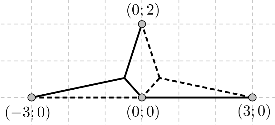 Figure 1
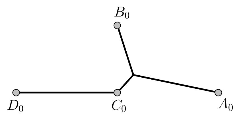 Figure 2
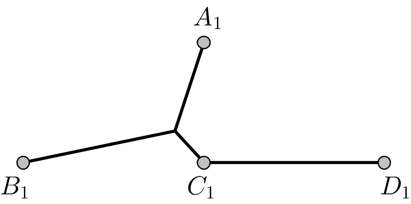 Figure 3
 Figure 4
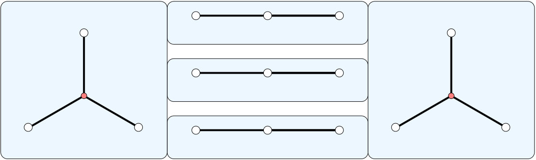 Figure 5
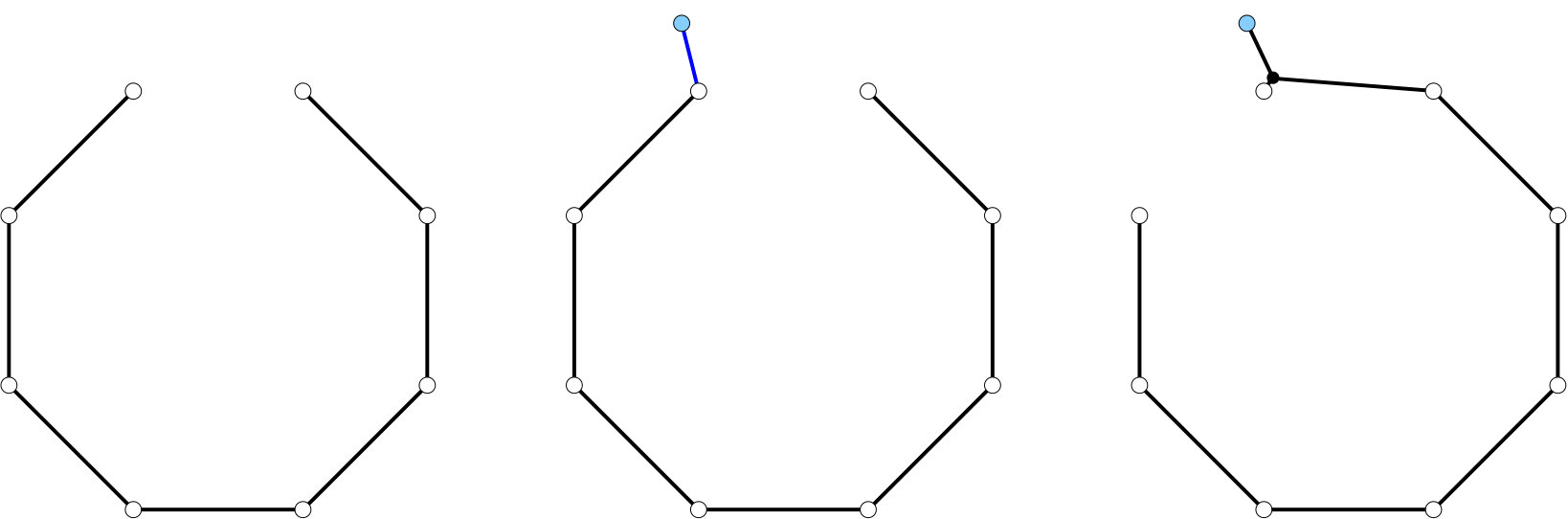 Figure 6
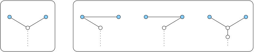 Figure 7
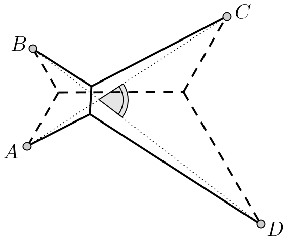 Figure 8
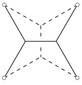 Figure 9
| ordered set of points in Euclidean space | |
|---|---|
| partially ordered connected graph | |
| network, graph; type | |
| network, graph; type | |
| homeomorphisms | |
| configuration, configuration space | |
| unambiguous cell, cell | |
| path | |
| time parameter, moment | |
| infinite sequence, index | |
| convergence, limit | |
| constant; bounded convex region | |
| vertices | |
| directions | |
| positive extensions | |
| supremum extension function | |
| motion vector, direction vector | |
| length, derivative | |
| angles |
Peer Reviews
No public reviews on file for this paper yet. If you reviewed it on a platform where reviews are public (OpenReview, ICLR, NeurIPS, ICML), you can paste yours below so the community can read it here.
Videos
No videos yet. Explain this paper in a talk, walkthrough, or lecture? Add one.
Taxonomy
TopicsComputational Geometry and Mesh Generation · Advanced Graph Theory Research · VLSI and FPGA Design Techniques
On the Configuration Space of Steiner Minimal Trees 111The authors acknowledge the support by the Russian Government through the mega project, resolution no. 220, contract no. 11.G34.31.0053.
H. Edelsbrunner222IST Austria (Institute of Science and Technology Austria), Klosterneuburg, Austria. and N. P. Strelkova333Moscow State University, Moscow, Russian Federation.
Abstract
Among other results, we prove the following theorem about Steiner minimal trees in -dimensional Euclidean space: if two finite sets in have unique and combinatorially equivalent Steiner minimal trees, then there is a homotopy between the two sets that maintains the uniqueness and the combinatorial structure of the Steiner minimal tree throughout the homotopy.
Keywords. Steiner minimal tree, shortest network, configuration space
05C05, 51M16
1 Introduction
Shortest networks connecting finite sets of geographic locations were intensely studied when the telephone providers were legally required to charge for phone calls an amount that is proportional to the length of the connection [3]. This motivated the discovery of many mathematical and computational properties of such networks. Nevertheless, many of the fundamental questions are still open. For example, in 1968 Gilbert and Pollak [7] conjectured that the ratio of the length of a minimum spanning tree over the length of a shortest network of the same point set cannot exceed . In 1992, Du and Hwang claimed a proof of the conjecture [4], but years later, Ivanov and Tuzhilin noted that there are gaps [11], and the problem remains open until today [13]. In contrast to the ratio problem, surprisingly little attention was directed toward the configuration space of the shortest networks, a topic we approach in this paper. Specifically, we consider a finite set of points, , in -dimensional Euclidean space, which we denote as . A spanning network of is a finite set of rectifyable curves, each connecting two points in but not necessarily in , whose union is connected and contains . We measure the length of the network using the Euclidean metric. A shortest network of is a spanning network of minimum length.
It is known to exist, and it satisfies the following properties; see e.g. [7]:
- •
it is a tree whose edges are straight line segments ending at vertices of degree , , or ;
- •
all degree- and degree- vertices are points in ;
- •
the angles between the edges meeting at a degree- vertex are , while the angle between the edges meeting at a degree- vertex is at least .
A shortest network of a finite set of points is usually referred to as a Steiner minimal tree. This tree may or may not be unique, and in the latter case, we call the Steiner minimal tree ambiguous. For example, the four corners of a square have two Steiner minimal trees; see Figure 1. Note that these two trees have different combinatorial structure if the points are labeled. Just to mention one difference: the points and are connected by a path of two edges in the solid tree, and by a path of three edges in the dashed tree. Suppose now that consists of four (arbitrary) points in the plane, and we need to find a Steiner minimal tree. If we know how many additional vertices there are in the tree, and how they are connected to the four given points and to each other, then we can locate them using the -condition. Generalizing this idea to points in the plane gives Melzak’s algorithm [14]. But a priori, we do not know which combinatorial structure gives the minimum length, and there is no known way that avoids checking all of them in the worst case. Indeed, the problem of constructing a Steiner minimal tree in is NP-hard even for ; see [6, page 209].
For a given finite set, , the collection of Steiner minimal trees of is well defined, and every tree in this collection has a different combinatorial type [7], a notion that will be made precise later. We are interested in the following question: for a given combinatorial type, what does the space of points whose Steiner minimal trees are of this type look like topologically? To make this more concrete, we order the points in and list the coordinates in sequence, mapping to a point in . For a given combinatorial type, we consider the space of points in that correspond to sets in with unambiguous Steiner minimal tree of the given type. Our main result is that this space is path-connected. We have a weaker result if we relax the requirement and allow ambiguous Steiner minimal trees. Here we can prove path-connectivity only for full networks in the plane. Finally, we exhibit an example to show that the space of points with necessarily ambiguous Steiner minimal trees of a given type is generally not connected. While the restricted setting for the result on cells is disappointing, it is consistent with a general lack of understanding of ambiguous Steiner minimal trees. For example, it is not known that the space of ambiguous Steiner minimal trees has measure zero. The only partial result is in dimensions, where the unambiguous Steiner minimal trees contain an everywhere dense open subset of the configuration space, but the proof in [12] is long and complicated. The approach in [15] leads to a shorter proof.
Outline.
Section 2 introduces the main concepts needed to formally state our results. Section 3 presents the key tools used in our proofs. Section 4 presents the proofs. Section 5 concludes the paper.
2 Concepts and Results
The two main concepts in this paper are the spanning networks of a set of points in , and the decomposition of the -dimensional configuration space into cells whose points have combinatorially equivalent shortest networks. We discuss both and introduce the terminology needed to formally state our results.
Graphs, networks, types.
Similar to the notion of a curve in differential geometry, we define a network as a map from an abstract topological to a concrete geometric space. In our context, the abstract space is a finite connected graph, . It is partially ordered, with ordered and unordered. The difference arises because the vertices in are mapped to the points in , which are ordered, while the vertices in can be mapped anywhere. To emphasize the difference, we sometimes call an element of a terminal vertex and an element of an interior vertex; an element of is an edge. Two partially ordered graphs, and , are combinatorially equivalent if there exist compatible bijections , , and of which the first preserves order. Observe that the preservation of order prevents the existence of such bijections for the two trees in Figure 1. We have , and since we are obliged to map to and so on, it is impossible to find a compatible bijection between the two edge sets.
We find it convenient to consider a graph as a -dimensional topological space, so it makes sense to talk about a point , which may be a vertex or a point on an edge of . If and are combinatorially equivalent, then there exists a consistent homeomorphism , that is: restricts to the bijections establishing the combinatorial equivalence. With this preamble, we introduce the first main concept.
Definition** 1****.**
A network is a continuous map such that the image of every edge is a rectifyable curve or a point, and the preimage of the image of every vertex is a subgraph of , possibly together with subsets of points on edges whose images happen to pass through this image. We call a parametrization of , and a contracting parametrization if every subgraph with constant image is connected.
The (combinatorial) type of is the graph obtained from by shrinking each subgraph with constant image to a vertex. Shrinking is similar to the contraction operation defined in Tutte [17, page 32] but more general because we do not require that the subgraphs that shrink to vertices be connected. The type is again a graph although it may have loops and multi-edges even if does not. The network spans an ordered set if restricts to an order-preserving bijection from to . To compare networks, we write for the sum of the lengths of the curves. A straight-line network maps every edge to a line segment or point. Of particular importance are shortest spanning networks, which are necessarily straight-line but also satisfy the three properties stated in Section 1. A Steiner minimal tree is the image of a shortest network. The image of a shortest network is necessarily a tree, so it is natural to parametrize it using a tree. In this case, the type is obtained by shrinking connected subtrees, so the parametrization is necessarily contracting.
The above definitions allow for different degrees of sameness between two networks, and . We call identical if are combinatorially equivalent and there is a consistent homeomorphism such that for every . Note that this is strictly stronger than requiring combinatorially equivalent graphs and equal images. A weaker and perhaps more natural notion calls the same if their types, , are combinatorially equivalent, and there is a consistent homeomorphism such that for every . For example, two shortest networks are the same iff they have the same Steiner minimal tree. Yet weaker is the notion that says have the same type if are combinatorially equivalent. In dimension , we require in addition that there is a homeomorphism such that . For plane embeddings, this is equivalent to requiring that the ordering of the edges around the vertices is the same in both images. While the three notions of sameness are different and relate to each other by a chain of implications, they are all transitive. We get the reverse chain of implications for the negations: having different type implies not being the same implies not being identical.
Configurations, cells, decompositions.
Let be an ordered set of points for . Listing the coordinates in sequence, we obtain a point
[TABLE]
We require that the points in are distinct, which implies that cannot lie on any of the -dimensional planes of the form , where we list the -th and the -th -tuple of coordinates, both specifying the same point in . Observe that all contain the diagonal of points . We use as the configuration space for sets of points in .
Definition** 2****.**
The cell of a type , denoted as , is the space of points that have shortest networks of type . The unambiguous cell of , denoted as , is the subspace of points such that has a unique Steiner minimal tree.
The remaining points, in , have at least two shortest networks, one of type and another of necessarily different type; see [7]. What can we say about the cells? Clearly, they cover the configuration space since every point has at least one shortest network. The cells have possibly non-empty intersections, and removing these intersections leaves us with the unambiguous cells, which are disjoint but do not necessarily cover the configuration space. As mentioned earlier, there is not much known about the space of points with ambiguous shortest networks. To complete the picture, we note that the points in the correspond to multisets, or after identification to sets of size in . We can therefore complete the decomposition of by partitioning the into strata within which is a constant, and to decompose each stratum according to shortest networks. By definition, the cells in these strata belong to the boundaries of the cells in , but not to the cells themselves.
We illustrate the decomposition of the configuration space with a small example: points in dimensions. There are only five different types, each generating a cell in ; see Figure 2. Factoring out the three dimensions of rigid motions, we may visualize the decomposition in the remaining dimensions. Drawing the diagonal as a point at the origin with three emanating half-lines for the , , we get a ring of three cells separating the two remaining cells. The origin lies in the boundaries of all five cells, while each half-line belongs to the boundaries of four. Only six of the ten transitions between the five cells avoid the origin and the half-lines, and we visualize them as -dimensional membranes, which lie in the common boundaries of the corresponding cells. In this particular example, these membranes belong to the three cells in the ring but not to the other two cells. For example, a point on the membrane separating the cell on the left from the cell at the center in Figure 2 has a Steiner minimal tree consisting of two edges that form an angle of at . The combinatorial type of this network is different from that on the left but the same as that at the center. Indeed, the two separated cells do not contain any points of their boundary, while the three cells in the ring contain every boundary point that does not belong to the origin and the half-lines.
Main results.
We are now ready to give formal statements of our main results. They state that unambiguous cells are connected for all dimensions , and that cells are connected for full networks in . In contrast, the difference between a cell and the corresponding unambiguous cell is not necessarily connected, which we will show by exhibiting an example of points in dimensions.
Theorem** 1****.**
(Connectedness of unambiguous cells)* Let be the type of a shortest network of a finite set of points in , for . Then is path-connected.*
Theorem** 2****.**
(Connectedness of cells)* Let be the type of a shortest network of a finite set of points in such that all terminal vertices have degree-. Then is path-connected.*
3 Tools
The proof of our main result is inductive, applying a procedure similar to Melzak’s algorithm; see [7, Section 5] or [14]. We begin by introducing the ingredients of the procedure, proving lemmas in preparation of the proofs of the theorems.
Locally minimal and pairs of codirected networks.
A network that satisfies the three properties stated in Section 1 is called locally minimal. Every shortest network is locally minimal but there are others; see Figure 3 for an example. As its name suggests, there are no shorter networks nearby, in which the notion of nearness is defined by parametrizing the networks by their interior vertices. More generally, it is not possible to have two locally minimal networks of the same type. We state this result for later reference; see [10, pages 927 and 939].
Proposition** 1****.**
(Uniqueness of minimal network)* Let be a partially ordered tree with terminal vertices and an ordered set of points in . If there exists a locally minimal network that spans and is parametrized by , then it is unique and the shortest such network.*
As a special case, we see that two different shortest networks of the same set that are parametrized by the same tree are impossible. A related concept is the following. Two straight-line networks, and , that span the same set are codirected if they look geometrically the same in the neighborhood of every vertex. More formally, we require that there exists such that the intersection of the ball with radius centered at with the images of and are the same for every terminal vertex . The existence of codirected locally minimal trees that are not the same is open, but in the plane it is known that such pairs do not exist [15].
Proposition** 2****.**
(Non-existence of codirected trees)* Any two locally minimal trees spanning the same ordered set of finitely many points in that are codirected are the same.*
Sequences of networks.
Another useful tool in the study of cells and their boundaries are converging sequences. We write for the networks in an infinite sequence, indexing them with the positive integers . In this paper, we are primarily interested in sequences such that the have all the same type, . We say such a sequence converges if the sequence of points converges for every vertex of . For straight edges, the limit of a converging sequence is well defined, namely the straight-line network such that for each vertex . We write as well as . Note that is not necessarily of type , but parametrizes by construction. An important method for obtaining converging sequences follows from the Bolzano-Weierstrass Theorem in analysis: starting with an infinite sequence of networks with finitely many types and points within a compact domain, we obtain a converging sequence by repeatedly restricting the choice and continuing the process with an infinite subsequence.
For straight-line networks, implies that the length of converges to the length of . It is therefore easy to see that if all are shortest networks, then is a shortest network with a contracting parametrization. Another important property of converging sequences of shortest networks is that convergence for the terminal vertices implies convergence for all vertices. In other words, as long as the shortest network does not change its type, it depends continuously on the points it spans.
Lemma** 1****.**
(Convergence of shortest networks)* Let be a tree, and let be a converging sequence of points in with shortest networks , all of type . Then is a converging sequence of networks, and the limit network is a shortest network of the limit of .*
Proof. Since converges, there exists a bounded and convex domain that contains the images of the terminal vertices of for all . The images of the interior vertices lie within the convex hull of the images of the terminal vertices and hence also in . We can therefore apply the Bolzano-Weierstrass Theorem and obtain a converging subsequence of shortest networks, with limit . To get a contradiction to the claimed property, we assume that does not converge to . Then there exists an interior vertex of , a constant , and an infinite subsequence such that for all . Applying the Bolzano-Weierstrass Theorem to this subsequence gives another converging sequence of shortest networks, now with limit . Thus, we get two shortest networks of the same set , both parametrized by the same tree . Both are locally minimal, which contradicts Lemma 1.
Note that Lemma 1 implies that every point in the boundary of has a shortest network parametrized by , and the parametrization is contracting.
Moustaches.
A particularly simple application of infinite sequences is used to shrink and grow edges of Steiner minimal trees that end at degree- vertices. Let be a shortest network of a set of points in , let be its type, and recall that it enjoys the three properties stated in Section 1. Hence, has at least one of the following two substructures: a two-sided moustache consisting of degree- vertices and both adjacent to a degree- vertex , or a one-sided moustache consisting of a degree- vertex adjacent to a degree- vertex . We call the anchor of the moustache in both cases. We shave a two-sided moustache by removing and together with the edges connecting them to . This leaves a smaller graph and a network that spans a smaller set of points, namely if , and union if . Similarly, we shave a one-sided moustache by removing together with the edge connecting it to . In this case, is necessarily in , so we get a spanning network of . Importantly, the operation preserves minimality in both cases. For later reference, we state and prove a slightly more general claim, namely that trimming a moustache preserves minimality.
Lemma** 2****.**
(Trimming a moustache)* Let be the type of a shortest network of a set of points in , let be a degree- vertex of and its neighbor. For , let be the same except that it maps to . Then is a shortest network of , and if is unambiguous then so is .*
Proof. Suppose there exists a network that spans with . Append the line segment from to to get a network that now spans . Then , which contradicts the assumption that is a shortest network of . The same argument contradicts the existence of different shortest networks for if there is only one for .
When we shave a moustache, we effectively map a point to a point in - or -dimensional configuration space, depending on the case. Doing this over all points and all moustaches of the corresponding shortest networks, we get multiple maps from higher- to lower-dimensional configuration spaces, each skipping either or dimensions. We will exploit the fact that every point in an unambiguous cell has plenty of preimages. In other words, if has an unambiguous shortest network, then we can grow a moustache while preserving that the network is shortest and unambiguous, of course now spanning a larger set . This property does not necessarily hold for sets with ambiguous shortest networks. Indeed, the corners of a regular octagon have eight different shortest networks [5], and none of them permits the growth of a one- or two-sided moustache such that the network remains shortest; see Figure 4.
Admissible extensions.
Before proving the property for unambiguous shortest networks, we introduce notation for adding a moustache. Let be a shortest network, let be a degree- vertex with neighbor in , and let be a direction. To add a two-sided moustache with anchor , we require that the angle between and the direction be . Equivalently, we require , and if this equation is satisfied, then we call an allowed direction for . For such a , there exists a unique second direction such that . Choosing , we construct . Similarly, we construct from by adding vertices and , connecting both with new edges to , and we construct such that the restriction to agrees with . We call admissible for and if is the unique shortest network of .
Adding a one-sided moustache is similar, except that is an allowed direction if , and there is no second direction to worry about.
Lemma** 3****.**
(Existence of admissible extensions)* For each unambiguous shortest network , each degree- vertex in , and each allowed direction , there exists such that every is admissible for and .*
Proof. We consider the two-sided case and omit the proof of the easier, one-sided case. Assume without loss of generality that is the type of , write for the ordered set of points spanned by , and let be the image of the anchor. We prove that the set of admissible extensions is not empty. Given a positive admissible extension, Lemma 2 then implies that all smaller extensions are also admissible, which gives the claimed statement. To get a contradiction, we assume that there is a degree- vertex of and an allowed direction , such that no is admissible for and . The plan is to construct two different locally minimal networks that are parametrized by the same tree. By Proposition 1, such networks do not exist, which will furnish the desired contradiction.
The first locally minimal network is obtained by growing a two-sided moustache of sufficiently small size to avoid self-intersections. Assuming is its type, we get from by adding vertices and and edges that connect them to . To construct the second locally minimal network, we use the assumption that there is no positive admissible extension. Choosing an infinite sequence that vanishes in the limit, we set and write for the shortest network of , letting be its type. Since we can select a converging subsequence, we may assume that for all , and that converges to a network . Since both and are shortest, they are the same, only with different parametrizations. To analyze this difference, we consider the preimage, .
We note that and are the only terminal vertices whose images converge to . All interior vertices of have degree , but one of them can have degree less than in , namely the endpoint of the edge that connects to the rest of the tree. There cannot be a second such vertex for this would contradict that has a contracting parametrization as implied by Lemma 1. Since has at most three vertices of degree less than , we are left with the choices shown in Figure 5. The tree on the very right can be used to reparametrize the other three. We can therefore reparametrize and with the same tree. Both networks are locally minimal and span the same set, , which contradicts that they are different.
Lower semi-continuity.
Fixing , we may consider the shortest networks of all and grow a moustache from the fixed anchor, , in each. Within each such network, we have a direction determined by the image of and the image of its neighbor, . By Lemma 1, depends continuously on . We can therefore choose an allowed direction, , that depends continuously on . The second direction, , needed to grow a moustache is uniquely determined by and . Let be defined by mapping to the minimum of and the supremum of the thresholds for which Lemma 3 holds. We do not know whether this function is continuous, but we can prove lower semi-continuity, which is sufficient to prove that the infimum of over a compact set of points is positive.
Lemma** 4****.**
(Lower semi-continuity)* Let , all points in a common unambiguous cell. Then .*
Proof. We consider the two-sided case and omit the proof of the easier, one-sided case. To get a contradiction, we suppose that for some . Choose a converging sequence such that for each . Writing for the set of points that corresponds to and for the image of the anchor, we introduce and let be the network obtained by adding the moustache to the shortest network of . Writing for the type of that shortest network, we get the type of from by adding vertices and and connecting them with edges to the anchor. Because , the constructed network is either not a shortest network or it is not unique. In either case, there exists a different shortest network spanning the same ordered set . Since we can choose subsequences, we may assume that the all have the same type . By Lemma 1, converges to a shortest network spanning . By construction, , so has a unique shortest network . This implies that and are the same. Networks of type can therefore be parametrized by . But then and are different locally minimal networks parametrized by the same tree, which contradicts Proposition 1.
4 Proofs
With the preparations in Section 3, we are now ready to prove Theorems 1 and 2, which have been formally stated at the end of Section 2. In addition, we illustrate the limitation of connectivity with an example.
Proof of Theorem 1.
Recall that this theorem asserts that unambiguous cells in the decomposition of the configuration space of points in are path-connected for all . We use induction over the number of points. For , there is only the trivial Steiner minimal tree, whose unambiguous cell is the entire , which is path-connected. For , there is again only one Steiner minimal tree consisting of two points connected by a line segment. The unambiguous cell is the entire minus the diagonal, which is a -dimensional plane. This space has the homotopy type of the -dimensional sphere. It is path-connected for all . This establishes the claim for and .
For the inductive step, we consider two points, and , in an unambiguous cell , and prove that there exists a path with and . Choose a moustache in , shave it, and write for the resulting smaller tree. This construction establishes a map from to , as described in Section 3. Note that is contained in or in , depending on the choice of moustache. By induction, is path-connected, which implies the existence of a path such that and are images of and under the map. We are going to lift the path to taking inverses. Lemma 3 states that we can find a preimage of for every . It remains to show that the preimages can be chosen in such a way that they give a path . But all the work needed to achieve this has already been done. As explained before Lemma 4, we can choose directions and that depend continuously on . It is easy to modify this direction field so that when we move along , we connect the needed directions at the two ends. Next, we set and note that because is compact, and is everywhere positive as well as lower semi-continuous; see Lemma 4. Moving along , we thus get a path consisting of networks with moustaches of uniform size. To get , we first trim the moustache to go from to , we second move from to , and we third enlarge the moustache to go from to .
Proof of Theorem 2.
Our second result asserts path-connectivity for cells, but only in dimension and for a full network in which all terminal vertices have degree . Suppose is a shortest such network for a set , let be its type, and let . Since we know that is path-connected, it suffices to construct a path that starts at and ends at a point . We prove the existence of such a path by considering the derivative of the length function. Write for the motion vector of , and define the direction vector by taking the sum of unit vectors in the directions of the incident edges:
[TABLE]
The first derivative of the length function in the direction of the motion is the sum of scalar products between motion and direction vectors. Since the direction vector of every interior vertex vanishes, this gives
[TABLE]
see [9, page 64]. We are interested in the special case in which for every . Then , the number of terminal vertices. Returning to the task at hand, we consider a second shortest network, of , and we compare the two derivatives. The vectors have at most unit length. This is immediate if the degree of in is , and it follows from the angle condition if the degree is . Hence, , with equality iff for all terminal vertices. If the difference is positive, then we move the points to for smaller than the length of the shortest edge of . After this motion, the adjusted network is shorter than the adjusted network .
It remains to show that vanishing difference is not possible. As mentioned, this is equivalent to for all . If all terminal vertices have degree , then this implies that and are codirected, which according to Proposition 2 is impossible for two shortest networks that are not the same. Otherwise, we grow a new edge from every vertex whose degree in is in the direction . We grow these edges both in and in . The two trees may no longer be shortest, but for sufficiently short extensions, they are both locally minimal. We thus get a contradiction from the stronger version of Proposition 2 which asserts that no two locally minimal trees can be codirected.
Example.
To complement our theorems, we show that ambiguous subsets of cells are not necessarily connected. Specifically, we exhibit an ambiguous shortest network of type such that is not connected. The network spans the ordered set of points in drawn in Figure 6. The two trees superimposed on the left are the only two Steiner minimal trees of the four points. Indeed, there cannot be a full Steiner minimal tree with two interior vertices because the four points do not form a strictly convex quadrilateral; see [16, Lemma 5], and the remaining types with one or zero interior vertices give longer networks.
For the next step, we choose two orderings of the four points such that the first Steiner minimal tree for the first ordering has the same type as the second Steiner minimal tree for the second ordering; see Figure 6 in the middle and on the right. We claim that there is no path from the first to the second tree along which the Steiner minimal tree remains of the same type and ambiguous at all times. To derive a contradiction, we suppose there is such a path . Consider the counterclockwise angle, , from the edge connecting to to the second edge incident on . Since we have a Steiner minimal tree at all times, we have for all . Taking a look at Figure 6, we see that and . Since depends continuously on , there is a value such that . At , the Steiner minimal tree is determined by the points . However, the Steiner minimal tree of three points cannot be ambiguous. This contradicts that is a path inside . We note that this example does not extend to dimensions.
5 Discussion
This paper continues the study of the decomposition of the configuration space of points in as defined by the combinatorial types of the Steiner minimal trees, which was initiated in [12]. We consider the ordered setting and our main result is a proof that the cells consisting of configurations with unambiguous Steiner minimal trees are path-connected. There are many questions that remain open.
- •
Can our partial results for cells be extended to all configurations in and to higher dimensions?
- •
Is it true that the set of points in with ambiguous shortest networks has measure zero?
- •
Is the non-empty intersection of two cells in necessarily path-connected?
- •
Is the union of sets in over all types path-connected?
Besides the ordered setting considered in this paper, it would be interesting to address the same questions for unordered point sets. The additional symmetries complicate the global topology [2], and more sophisticated notions of connectivity as offered by homology and homotopy groups seem appropriate.
Acknowledgments.
The authors thank A. O. Ivanov, Z. N. Ovsyannikov, and A. A. Tuzhilin for insightful discussions on the contents of this paper.
Appendix A Notation
Appendix B Dependence
The reference list from the paper itself. Each links out to its DOI / PubMed record.
- 1[1]
- 2[2] J. S. Birman. Braids, Links, and Mappings. Princeton Univ. Press, Princeton, New Jersey, 1974.
- 3[3] X. Cheng, Y. Li, D.-Z. Du and H. Q. Ngo. Steiner trees in industry. In Handbook of Combinatorial Optimization, Vol. 5 , eds.: D.-Z. Du and P. M. Pardalos, 193–216, Kluwer Academic Publ., 2004.
- 4[4] D.-Z. Du and F. K. Hwang. A proof of Gilbert-Pollak conjecture on the Steiner ratio. Algorithmica 7 (1992), 121–135.
- 5[5] D.-Z. Du, F. K. Hwang and J. F. Weng. Steiner minimal trees for regular polygons. Discrete Comput. Geom. 2 (1987), 65–84.
- 6[6] M. R. Garey and R. L. Johnson. Computers and Intractability. A Guide to the Theory of NP-Completeness. Freeman and Company, San Francisco, California, 1979.
- 7[7] E. N. Gilbert and H. O. Pollak. Steiner minimal trees. SIAM J. Appl. Math. 16 (1968), 1–29.
- 8[8] F. K. Hwang. A linear time algorithm for full Steiner trees. Oper. Res. Lett. 4 (1986), 235–237.