A minimal model for slow, sub-Rayleigh, super-shear and unsteady rupture propagation along homogeneously loaded frictional interfaces
Kjetil Th{\o}gersen, Henrik Andersen Sveinsson, David Sk{\aa}lid, Amundsen, Julien Scheibert, Fran\c{c}ois Renard, Anders Malthe-S{\o}renssen

TL;DR
This paper introduces a minimal, two-parameter model for various rupture front types along frictional interfaces, revealing that diverse rupture behaviors are inherent to velocity-strengthening frictional systems.
Contribution
The study presents a simple yet comprehensive model capturing multiple rupture front modes using only two key parameters, advancing understanding of frictional rupture dynamics.
Findings
Model reproduces slow, sub-Rayleigh, super-shear, and unsteady rupture fronts.
Diverse rupture behaviors are inherent to velocity-strengthening friction.
Model highlights the role of prestress and viscosity in rupture dynamics.
Abstract
In nature and experiments, a large variety of rupture speeds and front modes along frictional interfaces are observed. Here, we introduce a minimal model for the rupture of homogeneously loaded interfaces with velocity strengthening dynamic friction, containing only two dimensionless parameters; which governs the prestress, and which is set by the dynamic viscosity. This model contains a large variety of front types, including slow fronts, sub-Rayleigh fronts, super-shear fronts, slip pulses, cracks, arresting fronts and fronts that alternate between arresting and propagating phases. Our results indicate that this wide range of front types is an inherent property of frictional systems with velocity strengthening branches.
Click any figure to enlarge with its caption.
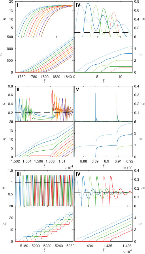 Figure 1
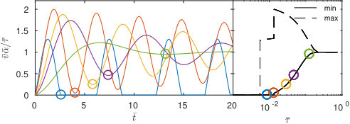 Figure 2
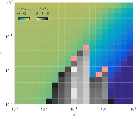 Figure 3
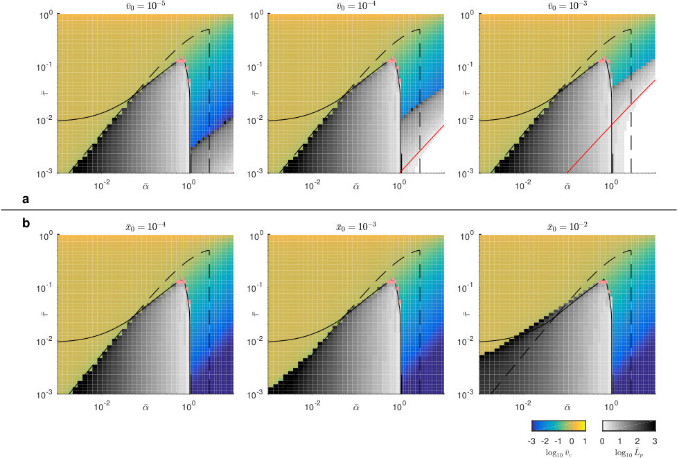 Figure 4
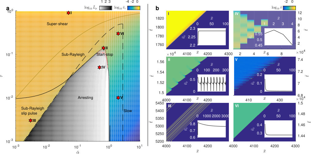 Figure 5
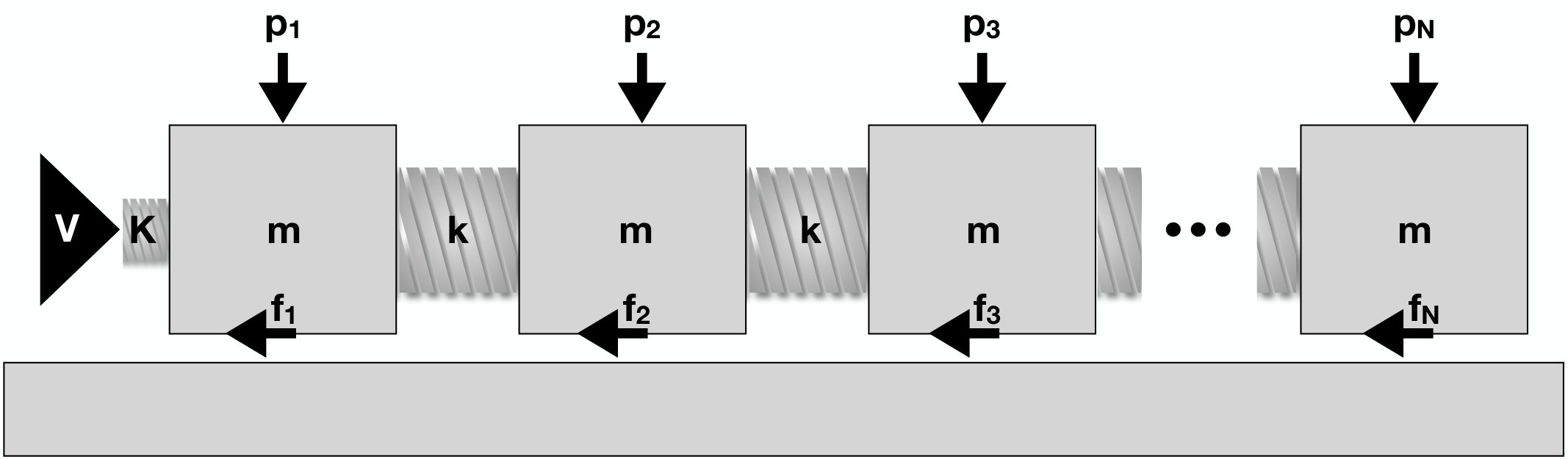 Figure 6
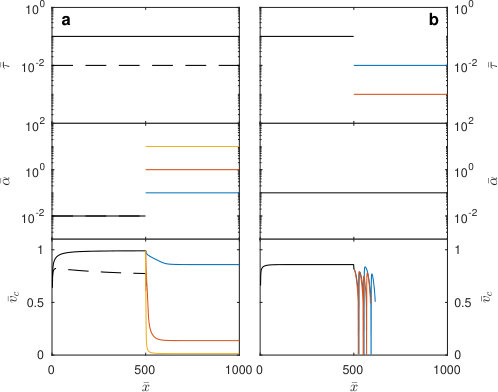 Figure 7
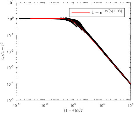 Figure 8
Peer Reviews
No public reviews on file for this paper yet. If you reviewed it on a platform where reviews are public (OpenReview, ICLR, NeurIPS, ICML), you can paste yours below so the community can read it here.
Videos
No videos yet. Explain this paper in a talk, walkthrough, or lecture? Add one.
A minimal model for slow, sub-Rayleigh, super-shear and unsteady rupture propagation along homogeneously loaded frictional interfaces
Kjetil Thøgersen
Henrik Andersen Sveinsson
David Skålid Amundsen
Julien Scheibert
François Renard
Anders Malthe-Sørenssen
Physics of Geological Processes, The NJORD Centre, University of Oslo, 0316 Oslo, Norway
Department of Geosciences, University of Oslo, 0316 Oslo, Norway
Department of Physics, University of Oslo, 0316 Oslo, Norway
Astrophysics Group, University of Exeter, EX4 4QL Exeter, UK
Univ Lyon, Ecole Centrale de Lyon, ENISE, ENTPE, CNRS, Laboratoire de Tribologie et Dynamique des Systèmes LTDS, F-69134, Ecully, France
University Grenoble Alpes, University Savoie Mont Blanc, CNRS, IRD, IFSTTAR, ISTerre, 38000 Grenoble, France
Abstract
In nature and experiments, a large variety of rupture speeds and front modes along frictional interfaces are observed. Here, we introduce a minimal model for the rupture of homogeneously loaded interfaces with velocity strengthening dynamic friction, containing only two dimensionless parameters; which governs the prestress, and which is set by the dynamic viscosity. This model contains a large variety of front types, including slow fronts, sub-Rayleigh fronts, super-shear fronts, slip pulses, cracks, arresting fronts and fronts that alternate between arresting and propagating phases. Our results indicate that this wide range of front types is an inherent property of frictional systems with velocity strengthening branches.
I Introduction
The onset of sliding of frictional contacts is often mediated by the propagation of a slip front along its interface, in natural, laboratory and industrial situations scholz1998earthquakes ; vakis2018modeling ; svetlisky2019brittle . Slip fronts typically nucleate at the weakest and/or most loaded part of the interface, propagate and eventually either invade the whole contact or arrest after breaking only a portion of the interface.
This front propagation can be characterized by two main features: front speed and front mode. Two main front modes have been identified, both in earthquakes and in laboratory experiments: Cracks where the interface behind the front slips until propagation ends rubinstein2004detachment ; xia2005laboratory ; ben2010dynamics ; latour2011ultrafast , and slip pulses where the ruptured part of the interface rapidly heals and re-sticks during propagation baumberger2002self ; lykotrafitis2006self ; nielsen2010experimental ; shlomai2016structure ; latour2011ultrafast . Propagation can occur at speeds differing by orders of magnitude; at velocities close to but below the Rayleigh wave speed (sub-Rayleigh), above the shear wave speed (super-shear), and at speeds orders of magnitude smaller than the sound speeds (slow). In addition, quasi-static fronts with a speed controlled by the external loading rate prevost2013probing have been reported. For dynamic cracks (from slow to super-shear, through sub-Rayleigh), higher propagation speeds are found for larger prestress of the interface ben2010dynamics and for larger dynamic stress drop svetlizky2017brittle . Such observations are not limited to experiments. In nature, earthquakes can propagate at both seismic and aseismic velocities burgmann2018geophysics , which obey different relations between seismic moment and earthquake duration ide2007scaling . Observations in nature also include periodic pulsing of aseismic events nadeau2004periodic .
When the propagation speed decreases to zero before a front reaches the edge of an interface, the front is denoted as arrested. Such fronts can be considered as precursors to sliding if they precede fronts spanning a larger portion of the interface rubinstein2007dynamics . The propagation length, like the propagation speed, depends on both the interfacial prestress and dynamic stress drop bayart2016fracture . Overall, the combination of the front mode, the range of its propagation speed and the information about whether it has arrested constitutes what we call the front type.
The range of observed front types have already been successfully reproduced by a variety of models. Arrested cracks have been reproduced using quasi-static models scheibert2010role ; braun2014propagation ; kammer2015linear ; bayart2016fracture , or elastodynamic models in 1D maegawa2010precursors ; amundsen20121d or 2D tromborg2011transition ; radiguet2013survival ; tromborg2014slow ; taloni2015scalar ; tromborg2015speed , assuming either continuous scheibert2010role ; maegawa2010precursors ; tromborg2011transition ; amundsen20121d ; radiguet2013survival ; taloni2015scalar or discrete-microcontact-based friction laws tromborg2014slow ; tromborg2015speed , or fracture concepts kammer2015linear ; bayart2016fracture . Slip pulses have been reproduced using discrete gerde2001friction or continuum models assuming either a Coulomb yastrebov2016sliding , regularized Coulomb andrews1997wrinkle ; cochard2000fault ; adda2003self or state-and-rate putelat2017phase ; brener2018unstable friction laws. Models of cracks are ubiquitous, featuring super-shear tromborg2011transition ; amundsen2015steady ; kammer2018equation , sub-Rayleigh tromborg2011transition ; radiguet2013survival ; bar2013instabilities ; tromborg2014slow ; tromborg2015speed , slow bouchbinder2011slow ; bar2012slow ; tromborg2014slow ; tromborg2015speed or quasi-static braun2009dynamics ; tromborg2014slow ; papangelo2015fracture fronts. Note that front speed has been shown to depend on many features of the frictional system, including slip history radiguet2013survival ; tromborg2015speed , interaction between different fault planes romanet2018fast , the shape of the high speed branch of the friction law bar2015velocity , and spatial heterogeneities in stress or constitutive parameters boatwright1996frictional ; bizzarri2001solving ; liu2005aseismic ; bruhat2016rupture ; helmstetter2009afterslip .
In front of so many different models, the physical origin of the observed richness in front types remains elusive. In this paper we address the question of the single minimal model that would reproduce the observed richness. We show how a simple friction model, reducible to only two non-dimensional parameters, contains a wide range of observed front types. Our findings indicate that the richness of front types is an inherent property of interfaces with velocity strengthening dynamic friction, which is a generic feature of both dry bar2014velocity and lubricated interfaces gelinck2000calculation ; olsson1998friction .
II Model description
We introduce a one-dimensional Burridge-Knopoff model burridge1967model for homogeneously loaded interfaces obeying Amontons-Coulomb friction, where the dynamic friction coefficient is velocity strengthening (Figure 1). The dimensionless equation of motion for sliding blocks is derived in appendix A and can be written as
[TABLE]
where is the dimensionless displacement. is the dimensionless prestress, where is the shear preload, is the normal load and and are the dynamic and static friction coefficients, respectively. is the dimensionless viscosity, where is the viscosity coefficient of the interface, is the spring constant between two blocks, and is the block mass. We select the dimensionless time and the dimensionless block separation so that the dimensionless speed of sound in the model is . We assume soft tangential loading (small driving velocity and small driving spring stiffness ), which results in boundary conditions given by a constant force on the leftmost block equal to its value when that block reaches its static friction threshold; . At the right boundary we keep block fixed; (appendix A).
Blocks start to move once the static friction threshold is reached, which in dimensionless units can be written as
[TABLE]
Blocks restick if the velocity changes sign.
The assumed friction law has a discontinuity at , because . Note that we investigated regularization of the model using either a characteristic length scale or a characteristic velocity scale (appendix D). The overall qualitative features of the model, in particular the various front types produced and their occurrence as a function of and , are the same as in the simple, unregularized model (Figure 8). At large slip velocities, we assume a velocity strengthening friction force, as is classical for both lubricated diew2015stribeck and dry interfaces bar2014velocity . The combination of a velocity weakening branch followed by a velocity strengthening branch as the slip velocity in increased is typical for Stribeck-like curves gelinck2000calculation ; olsson1998friction .
We emphasize that the present model can be fully described using only two dimensionless numbers: the dimensionless viscosity, , which defines the velocity strengthening term and the prestress , which indicates how close the interface is to its static friction threshold.
III Richness of slip and rupture
We have performed simulations for and to obtain the relationship between prestress, viscosity and front velocities shown in Figure 2. To reduce the computational cost we have performed for , with and for with (the transients in the large regime require a smaller propagation distance before steady state is reached). The simulations were run until all blocks stopped or the front reached the end.
III.1 Front speed
For each simulation, we have measured the steady state velocity for fronts progagating through the entire interface (colorscale in Figure 2a). To obtain steady state front velocities, we measure the times of rupture of all blocks, and extrapolate linearly to using the last 20% of the blocks. For arresting fronts, we measure the propagation length . The results are shown in Figure 2, with corresponding slip and velocity curves for the examples shown in Figure 3. The front velocities span a continuum from slow velocities for low and large to super shear-velocities at large and low . The front velocity at can be found analytically and is given by amundsen2015steady
[TABLE]
To estimate the steady state propagation speed in the limit of large , we start with the steady state slip speed, which can be obtained directly from equation 1. If the slip speed is constant, then , and , so that equation 1 reduces to , where the steady state slip speed is
[TABLE]
In the limit of large we expect the propagation speed to be governed by the steady state slip speed. If block has just ruptured, the displacement necessary to trigger the rupture of block is ( and in equation 2). The dimensionless distance between the blocks is . At a speed of it takes a dimensionless time to travel the dimensionless distance , so that the front speed is
[TABLE]
In Figure 4 we use equations 3 and 5 and find that we obtain a decent data collapse of the steady state front velocities when we plot against . From this collapse we obtain an empirical approximation of the front propagation velocity which is valid in both limits
[TABLE]
Inserting for the dimensional quantities in equations 3 and 5, we find the following dependencies on the density :
[TABLE]
From this we can immediately conclude that fast fronts are dominated by inertia while slow fronts are not. We emphasize that this separation between inertial and non-inertial fronts only apples to the end-member solutions of equation 6, and does not apply for the intermediate front velocities (found for large and in Figure 2).
III.2 Front type
We observe that the model is able to produce a large variety of front types. In addition to sub-Rayleigh, super-shear, and slow cracks, we observe slip pulse solutions, arresting fronts, as well as rupture speeds that alternate between propagating and arresting phases. Figure 2 contains boundaries of the different front types, as well as examples of space-time development of each front type. The corresponding local slip and slip speed for the examples in Figure 2 is shown Figure 3.
The sub-Rayleigh and super-shear front velocities are found in the limit of small , or large combined with large . The front velocities systematically increase with increasing . Examples of sub-Rayleigh and super-shear propagation is found in Figure 2bI and Figure 2bVI, with corresponding slip profiles found in Figure 3I and Figure 3VI. The slow fronts are found in the limit of large and small . An example of a slow front is shown in Figure 2bV with the corresponding slip profiles found in Figure 3V.
We also observe a large region in where steady-state solutions do not exist (greyscale in Figure 2). For these arresting fronts we measured the propagation distance , which increases with decreasing . There is also a sharp transition from fronts that stop within a small distance and the slow regime where steady state-solutions exist close to .
Slip pulse solutions in the Burridge-Knopoff model typically manifest as a series of slip bands, each a few blocks wide, propagating at the same velocity. The steady state slip pulse-region is found for small and small , but the arresting region also contains slip pulse solutions. An example of a slip pulse is shown in Figure 2bIII, with the corresponding slip profiles in Figure 3III.
We also observe front propagation that alternates between propagating and arresting phases, which we denote as start-stop fronts. The mechanism behind this front type is as follows: If a crack that is arresting is sufficiently long, it will always be able to restart as long as all blocks behind the front are still sliding. If a block at the front of a propagating crack arrests at position , the block in front of it will carry a stress of , where corresponds to the static friction threshold. There is thus a possibility for a force to be carried by two arrested blocks at the front tip. Restarting the propagation requires that there is sufficient force available in the form of slow slip behind the front tip. The available force can be written as where is the position of the front tip at the time of arrest. The criterion for the existence of a start-stop front can be found by balancing these two contributions; . The criterion for the unconditional restart of a crack that has arrested is found when , which corresponds to a stress close to the static friction threshold on the two arrested blocks in front of the crack. This can be written as a crack length that allows for the existence of start-stop fronts
[TABLE]
Note that this argument requires that the entire interface behind the front tip is sliding, which means that slip pulses will not be subject to this behavior. The start stop fronts are marked with a pink contour in Figure 2a and an example is shown in Figure 2bII with the corresponding slip profiles found in Figure 3II, and the measured is taken as the propagation length when the front stops for the first time ().
III.3 Phase diagram boundaries
In the following, we investigate the boundaries between the different front types observed in Figure 2a.
First, we find the line of unconditional propagation in Figure 2 (dashed), which separates the slip pulse region from the arresting region at small and then divides the sub-Rayleigh region for larger . If a block at the front tip is able to trigger the next block even though the block behind it has stopped, a propagating front will not be able to arrest. Solving for this criterion in and gives a criterion above which steady state propagation will always occur. The condition of the existence of such solution can be found analytically (appendix B) and is given as
[TABLE]
To obtain the arresting domain of the phase diagram, we need to determine when blocks in the system are able to reach zero velocity. This can occur during very short transients or because a steady state solution contains large velocity fluctuations. We have not been able to determine this criterion analytically, but it is straightforward to find the criterion numerically. Blocks can either stop at the front tip as in Figure 3IV, or because of velocity oscillations behind the front, as demonstrated in Figure 5. For a fixed , varying systematically changes the amplitude of such oscillations, which leads to a well defined criterion for the existence of arresting blocks . The procedure for determining the criterion is as follows: We use a system of blocks. For a given and , we run a simulation and check whether it contains blocks that start and then arrest before the front reaches the end. We then use the bisection method for fixed , varying to find the limiting .
This solution is plotted as a solid black line in Figure 2.
The two criteria and combined explains both the region of the phase diagram where steady state slip pulse solutions exist and the location of the arresting region. Steady state slip pulses exist in for , where velocity oscillations can lead to arresting blocks, but where propagation will continue even if blocks behind the front arrest. The arresting region is determined by .
III.4 Heterogeneous interfaces
The front type phase diagram of Figure 2a has been constructed from steady-state data. Here we investigate to what extent it can be used to understand some features of fronts propagating along heterogeneous interfaces. Figure6 illustrates that transitions in and can act as barriers to propagation, which can be understood from Figure 2a.
Changes in can lead to arresting fronts if a front initiated in a region of corresponding to steady state propagation enters a region corresponding to the arresting regime. This is demonstrated in the Figure 6b, where fast cracks entering regions of smaller arrest. In such cases, the criterion for start-stop fronts in equation 9 may be satisfied in the arrest phase, leading to multiple start-stop events before the motion stops completely. This is visible as velocity fluctuations after in the bottom row of Figure 6b. As shown in Figure 6a (dashed lines), if a front is initiated in the slip-pulse regime and then enters a region of larger crossing (equation 10), it will arrest even if the region of larger corresponds to slow rupture. In the simulations in Figure 6a, this arrest occurs within a few blocks. This means that a propagating front entering a region of different can arrest even though each value of would allow for a steady state propagation on a homogeneous interface. For larger where the entire interface is sliding when the region of increased is reached (Figure 6a, solid lines), the front speed converges to a new value corresponding to the values of and in that region of the phase diagram.
IV Discussion
In this paper, we have demonstrated that a minimal one-dimensional model of rupture along frictional interfaces, obeying Amontons-Coulomb friction with velocity-strengthening dynamic friction, contains the main front types observed in the physics and geophysics literature. This includes cracks, slip pulses and arresting fronts with steady state propagation speeds ranging from slow, to sub-Rayleigh and super-shear velocities. In addition to these steady state velocities, we observe fronts that alternate between arresting and propagating phases. This model can be written in terms of only two non-dimensional parameters that determine the front type. Complexity and richness of frictional rupture has been demonstrated to depend on different parameter ranges, boundary conditions, as well as spatial heterogeneities in stress constitutive parameters boatwright1996frictional ; bizzarri2001solving ; liu2005aseismic ; bruhat2016rupture ; helmstetter2009afterslip . We emphasize that the observed complexity and richness of frictional rupture in this study occurs on interfaces that are homogeneous in both frictional properties and loading. This highlights that the large variation in modeled front types are likely generic features of frictional interfaces with velocity strengthening dynamic friction.
An important question is whether those results are robust against qualitative changes in the model; in particular whether there are specific effects related to the discontinuity of the friction law at vanishing slip speed. We have performed two additional sets of simulations using regularized friction laws; one with a velocity-weakening and one with a slip-weakening regularization. The corresponding equations of motion and the associated steady-state front type phase diagrams are presented in appendix D. Comparison between the phase diagram in Figure 2a and the regularized models in Figure 8 indicates that most qualitative features are essentially unchanged. While some differences may be noted (details in appendix D), the spatial organization of the various regions in the phase diagram remains largely unchanged, showing that the discontinuity of the friction law does not change our main conclusions.
We have also performed a set of two-dimensional simulations to address whether our results would be specific to the 1D nature of the system. We combine the bulk model of tromborg2011transition with the present friction law. The parameters used and the results obtained are presented in Appendix C. The obtained phase diagram (Figure 7) is again similar to Figure 2a, which demonstrates that our main conclusions are not artefacts of the 1D nature of the model.
The relative locations of the various regions in Figure 2 are consistent with experimental observations. At low and , the model predicts the existence of slip pulse solutions, in agreement with the experimental observation that slip pulses occur when the prestress is low compared to the static friction threshold nielsen2010experimental . For , the model only predicts super-shear rupture amundsen2015steady . For non-zero , sub-Rayleigh and slow rupture can occur. Super-shear rupture can still occur if the prestress is large. Overall, the propagation speed increases with increasing prestress, which is consistent with experimental observations ben2010dynamics . Slow fronts have also previously been reported to depend strongly on velocity strengthening friction bar2013instabilities ; bar2015velocity . Here, slow propagation occurs at large . Both the slip speed and the slow propagation speed are directly controlled by the velocity strengthening term , leading to a slow propagation speed inversely proportional to .
In addition to steady state rupture, the model predicts unsteady rupture velocities, where a crack alternates periodically between sub-Rayleigh speed and a transient arrest. Restarting arrested cracks requires that sufficient slow slip occurs in the broken part of the interface. Intermittent rupture then continues as long as the slow slip endures. A similar mechanism was found to control the transition from fast to slow rupture in a multi-asperity model tromborg2014slow , reproducing observations in laboratory experiments rubinstein2004detachment . We also speculate that the start-stop regime found in this study may be an analog to observed periodic pulsing of aseismic events have been observed nadeau2004periodic .
In real systems, the prestress can vary largely depending on the boundary conditions. For side driven systems, the stress at the interface after a rupture has passed is likely to coincide with the dynamic friction level amundsen20121d ; tromborg2011transition , which corresponds to . This assumption is consistent with the observation in continuum rate-and-state models that the velocity corresponding to the minimum friction force sets the steady state slip speed and thus the rupture velocity bouchbinder2011slow . In our simulations, this minimum is located at zero velocity. However, the possibility of a prestress that can be larger than the dynamic level leads to a large variety of possible rupture speeds.
Several mechanisms can be responsible for varying stress conditions on frictional interfaces. Romanet et al. romanet2018fast showed that the interaction between two fault planes can lead to the co-existence of sub-Rayleigh and slow rupture on the same fault. Interactions between fault planes could lead to large variations in the stress conditions of the fault planes prior to rupture. This is consistent with our findings for large , where variations in alone can lead to propagation speeds ranging from slow, through sub-Rayleigh to super-shear.
Heterogeneities of the interface can also be due to spatial variations in the stress conditions or frictional properties. For instance, viscous patches along frictional interfaces have been shown to act as barriers to propagation because they can inhibit fast slip nielsen2010experimental . Similarly, in our simulations, changes in and along a frictional interface can cause rupture fronts to continue with a different velocity, or arrest, depending on whether the initial front propagates as a crack or a slip pulse, and on the region of the phase-diagram that the new value of and corresponds to.
Our simulations show a region where rupture fronts will arrest, even when . At low , this region causes a clear separation between sub-shear and slow rupture regions. In nature, observations show that fast and slow rupture obey different scaling relations between seismic moment and earthquake duration ide2007scaling . There is currently an ongoing debate about whether there should exist a continuum of scalings between these two end-members ide2007scaling ; peng2010integrated . For prestress close to the dynamic threshold where , the arresting region in and could inhibit observations of intermediate rupture velocities, in turn causing observations of earthquake rupture mainly in the fast and slow end members.
V Conclusion
In this paper, we have demonstrated that a minimal model of homogeneously loaded interfaces containing only two dimensionless parameters reproduces a wide range of observed slip and rupture behavior. This includes arresting fronts, slip pulses, unsteady rupture velocity, slow slip and rupture, fast rupture and super-shear rupture. Our results indicate that richness of frictional rupture is an inherent property of frictional systems with velocity strengthening dynamic branches.
Acknowledgements.
K.T acknowledges support from EarthFlows - A strategic research initiative by The Faculty of Mathematics and Natural Sciences at the University of Oslo. H.A.S acknowledges support from the Research Council of Norway through the FRINATEK program, grant number 231621.
Appendix A Equations of motion
The equation of motion for the one-dimensional Burridge-Knopoff model with a viscous term is
[TABLE]
where is the block index, is the displacement, is the mass, is the spring constant is the viscosity coefficient, the blocks are separated by a distance , and is the friction force. obeys Amontons-Coulomb law of friction, where a block begins to move when the static friction force is reached. When moving, the friction force is . A block arrests when changes sign. Now assume that all blocks are initialized with positions . Any additional movement can be described by
[TABLE]
Combining equation 11 and 12 yields
[TABLE]
where we have introduced the prestress
[TABLE]
We then define the dimensionless variables , and so that
[TABLE]
where the derivative is now taken with respect to . Selecting
[TABLE]
we obtain
[TABLE]
where
[TABLE]
where corresponds to .
For most of this paper, we consider homogeneous interfaces (, , ) and homogeneous prestress (, ). We also assume that the propagation is in the positive direction. This means that we set and , obtaining equation 1. Note that means that equation 1 is only valid for both positive and negative velocities in the special case when . A small portion of the simulations we perform will contain oscillations with negative velocities (far) behind the front tip, and these results are thus only strictly valid under the assumption . We have checked that this choice does not affect the propagation speed, but the detailed dynamics behind the front could depend on . The constraint results in the existence of steady state propagation only when . The choice of also ensures that a dimensionless front propagation speed of corresponds to the velocity of sound in the system
[TABLE]
Next, we set the boundary conditions. Block ruptures when the friction force reaches the static friction threshold. If the system is driven by a spring with spring constant driven at velocity , this corresponds to adding a force on block 1, which in dimensionless units becomes , where and is the time when the first block reaches the static friction threshold. For soft tangential loading , this boundary condition is reduced to .
In the Burridge-Knopoff model, the elastic modulus is given by , where is the cross-sectional area of the blocks. The mass density is defined as , which we make use of in the main text.
Appendix B Criterion for the unconditional existence of steady state propagation
If a block at the front tip is able to trigger the next block even though the block behind it has stopped, a propagating front will not be able to arrest. This criterion can be formulated as follows: The minimum criterion in for the existence of a steady state propagation is that a block stops at exactly , corresponding to the static friction threshold of the next block, thus triggering it. This assumptions translates to , , , . From equation 1 we find
[TABLE]
which has the solution
[TABLE]
From the assumptions and we find
[TABLE]
where we have assumed that the system is underdamped (). From we have
[TABLE]
where is the time at which the block position reaches . The requirement of zero velocity at can be found from
[TABLE]
where we are looking for the first non-trivial solution
[TABLE]
Inserting for in equation 23 we obtain
[TABLE]
which gives us the line of unconditional propagation in the phase diagram of and , as shown in Figure 2.
Appendix C Two-dimensional simulations
Here we address whether our results would be specific to the 1D nature of the system. We performed a set of simulations in 2D with the spring-block model described in tromborg2011transition . We simulate a slider of dimensions m, with blocks. We use friction coefficients and , and a varying velocity strengthening term . We use a Young’s modulus GPa, density kgm*-3*, width m, with a bulk damping coefficient of . To limit wave reflections from the top surface, we use a damping term at the top blocks. The normal force on the bottom blocks is prescribed to kN per block, and the system is initialized with a prestress , and the slider is pushed from all blocks on the left interface. The system is solved using adaptive time-stepping and event detection for the transition from static to dynamic friction. The simulations are run until all blocks have ruptured or all blocks have arrested.
Figure 7 shows the resulting front velocities, which confirm that the qualitative behavior from the one-dimensional still remains in two dimensions, and that the main conclusions are not artefacts of the one-dimensional nature of the model.’
Appendix D Regularization of the friction law
An important question is whether the results from the main text are robust against qualitative changes in the model. In particular, one may first ask whether there is any specific effect related to the discontinuity of the friction law at vanishing slip speed, when the frictional resistance on a block abruptly drops from the static friction force to the dynamic friction force. To answer the question, we performed two additional sets of simulations, using regularized friction laws: one with a velocity-weakening and one with a slip-weakening regularization.
First, we introduce a velocity scale for the decay from static to dynamic friction so that the equation of motion for sliding blocks can be written as
[TABLE]
where is a characteristic velocity scale that we vary. The resulting front velocities and propagation lengths are shown in Figure 8a. The main effect of the velocity regularization is that it introduces a minimum in the friction law that gives a minimum that allows for steady state propagation. For this criterion, which is the main cause of arresting in the large regime, we can immediately set up the expression
[TABLE]
This line is shown in red in Figure 8. No steady state can exist below this curve.
We also perform regularization with a displacement dependent term, which results in the following equation of motion:
[TABLE]
where is the displacement of block since the last time it ruptured. As can be seen in Figure 8b, the phase diagram is essentially unaffected by the regularization for small . For larger , the slip weakening regularization induces a widening of the arresting region at small values when the characteristic slip distance large. In those cases, the main effect is to shrink the region where slip pulses are allowed, making them more difficult to identify as a potential front type in the model.
Comparison between the phase diagram of the main model (Figure 2a) and that of the regularized models (Figure 8) indicates that most qualitative features are essentially unchanged. In particular, the spatial organisation of the various regions (front types) in the phase diagrams are unchanged, showing that the discontinuity of the friction law does not change our main conclusions.
The reference list from the paper itself. Each links out to its DOI / PubMed record.
- 1(1) Scholz, C. H. Earthquakes and friction laws. Nature 391 , 37 (1998).
- 2(2) Vakis, A. I. et al. Modeling and simulation in tribology across scales: An overview. Tribology International 125 , 169 – 199 (2018).
- 3(3) Svetlizky, I., Bayart, E. & Fineberg, J. Brittle fracture theory describes the onset of frictional motion. Annual Review of Condensed Matter Physics 10 , 253–273 (2019).
- 4(4) Rubinstein, S. M., Cohen, G. & Fineberg, J. Detachment fronts and the onset of dynamic friction. Nature 430 , 1005 (2004).
- 5(5) Xia, K., Rosakis, A. J., Kanamori, H. & Rice, J. R. Laboratory earthquakes along inhomogeneous faults: Directionality and supershear. Science 308 , 681–684 (2005).
- 6(6) Ben-David, O., Cohen, G. & Fineberg, J. The dynamics of the onset of frictional slip. Science 330 , 211–214 (2010).
- 7(7) Latour, S. et al. Ultrafast ultrasonic imaging of dynamic sliding friction in soft solids: The slow slip and the super-shear regimes. EPL (Europhysics Letters) 96 , 59003 (2011).
- 8(8) Baumberger, T., Caroli, C. & Ronsin, O. Self-healing slip pulses along a gel/glass interface. Physical review letters 88 , 075509 (2002).