Possibility of suppression of the formation of solute-enriched clusters
A.V. Subbotin, M.I. Gurevich, A.A. Kovalishin, P.A. Likhomanova

TL;DR
This paper explores a method to suppress solute-enriched cluster formation in irradiated pressure vessel steels by light alloying, altering solidification mechanisms, and preventing cluster formation in specific steel types.
Contribution
It introduces a novel approach of light alloying with selected elements to inhibit solute-enriched cluster formation during irradiation.
Findings
Suppression of cluster formation through alloying with elements of specific properties.
Alteration of solidification mechanisms to prevent solute drag.
Applicability limited to B.C.C. steels, not F.C.C. steels.
Abstract
Based on the earlier proposed mechanism of formation of solute-enriched clusters in irradiated pressure vessel steels, it has been demonstrated that it is possible to suppress this process by the method of light alloying of PVS with a chemical element with specially selected properties such as solubility, activity, and mobility. It is shown that it is possible to change the thermal spike molten zone solidification mechanism and suppress the "solute drag" leading to the formation of solute-enriched clusters. It must be noted that such a solute-enriched cluster formation mechanism is appropriate for alloying elements with low solubilities - it fits for B.C.C. steel-metal of PVS, but does not for the F.C.C. austenitic steels.
Click any figure to enlarge with its caption.
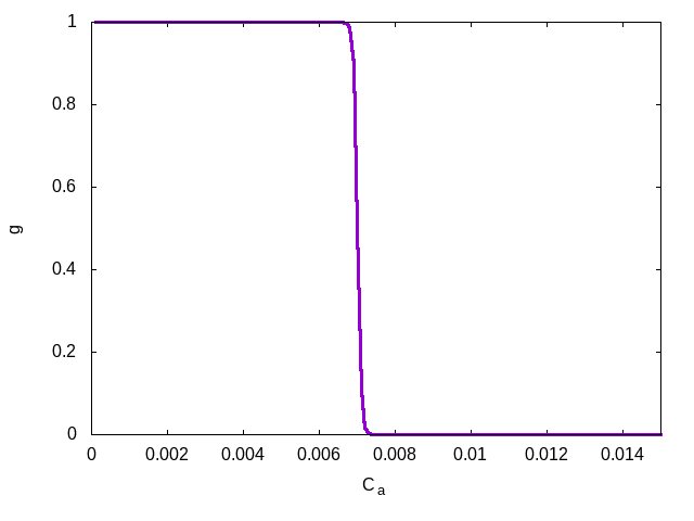 Figure 1
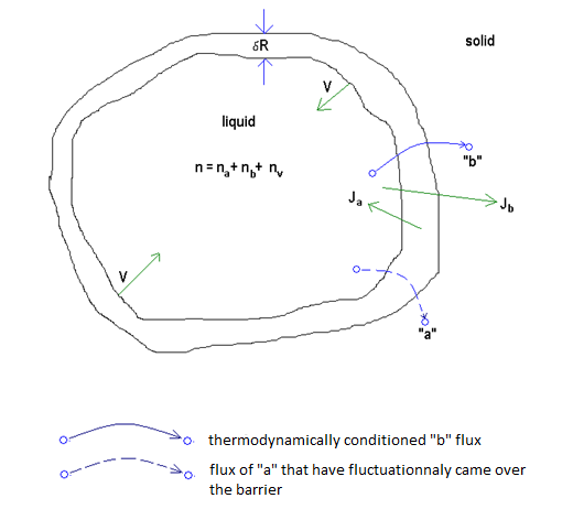 Figure 2
 Figure 3
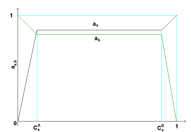 Figure 3
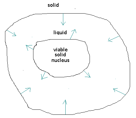 Figure 5
Peer Reviews
No public reviews on file for this paper yet. If you reviewed it on a platform where reviews are public (OpenReview, ICLR, NeurIPS, ICML), you can paste yours below so the community can read it here.
Videos
No videos yet. Explain this paper in a talk, walkthrough, or lecture? Add one.
Taxonomy
TopicsCrystallization and Solubility Studies
Possibility of suppression of the formation of solute-enriched clusters
A. V. Subbotin, M. I. Gurevich, A. A. Kovalishin, P. A. Likhomanova
NRC ’Kurchatov Institute’, 123182, Russia, Moscow, Academician Kurchatov Square, 1 CONTACT Email: [email protected]
Abstract
Based on the earlier proposed mechanism of formation of solute-enriched clusters in irradiated pressure vessel steels, it has been demonstrated that it is possible to suppress this process by the method of light alloying of PVS with a chemical element with specially selected properties such as solubility, activity, and mobility. It is shown that it is possible to change the thermal spike molten zone solidification mechanism and suppress the "solute drag" leading to the formation of solute-enriched clusters. It must be noted that such a solute-enriched cluster formation mechanism is appropriate for alloying elements with low solubilities—it fits for B.C.C. steel-metal of PVS, but does not for the F.C.C. austenitic steels.
K****eywords solute-enriched clusters, thermal spike, solute-liquid interface, solubility, nucleation, non-linear diffusion equation, boundary conditions
1 Introduction
In the present study, we continue the consideration of one of the two processes causing radiation-induced embrittlement of PWR-type reactor vessel steels, namely grain body hardening[1], [2], [3], [4], [5]. Through numerous experimental studies, it was concluded that radiation-induced generation of small-sized ( nm) quasi-spherical clusters enriched with solute elements , and considerably contributes to radiation-induced grain body hardening [6], [7], [8].
Reference [9] proposed and partly explicated the radiation-induced generation mechanism of solute-enriched cluster ensembles, which involves several stages.
) Thermal Spike Stage
Upon interaction with the lattice, a neutron with sufficient energy generates a primary knocked-on atom (PKA), which in its turn produces a collision cascade and a residual energy dissipation zone. Thermalization results in the generation of a thermal spike in a highly overheated (up to a temperature , where is melting temperature) localized zone for s. The PKA energy interval
is limited by the possibility of molten zone generation (for the lower limit) and the subcascading process (for the upper limit), and is interesting on account of the following considerations.
) Molten Zone Evolution Stage
A viable liquid phase nucleus can appear as a result of a fluctuation produced in the overheated zone and quickly grow to sizes conditioned by the thermal spike dispersed in the space. The condition for the stoppage of the development of the molten zone is
where is the maximum radius of the molten zone; is the thermal spike zone radius, with ; is the duration of development of the molten zone.
The duration of liquid phase generation corresponding to the typical parameters of the thermal spike does not exceed s.
) Solidification and Solute Drag
The thermal spike and the molten zone contained in it are present in the surrounding medium (metal) that has the temperature
Natural dispersion of the thermal spike suggests that the thermal spike zone () should begin contracting fast and become smaller than the molten zone. In reality, contraction of the zone corresponding to is mainly determined by the thermal conductivity. The molten zone contraction (sol-liq boundary motion) is governed by the mechanism of atom-by-atom liquid phase connection to the solid phase, where the main parameter is the atomic diffusion coefficient in the liquid phase, which is approximately two orders lower than the thermal conductivity coefficient. It indicates that the sol-liq interface must lag the interface, and the molten zone attains the purely undercooled condition.
Even considering the energy released at the sol-liq interface as the melting enthalpy, numerical solution of the corresponding equation of conductivity reveals that the entire molten zone attains the undercooled condition at for times s (where ) [10].
Further evolution of the molten zone in the undercooled condition can result in different scenarios, depending on the liquid phase composition.
In effect, the development of the liquid phase depends on the competition between two processes:
Solidification by way of the solid phase absorbing atoms from the liquid phase—this process is characterized by smooth (i.e. without any discontinuity) movement of the sol-liq interface till the end of the process. In this case, the lifetime of the liquid phase is determined by the relation
where depends on the near-interface concentrations of the solute ”” and of the solvent ”” in the equation for the liquid phase boundary motion rate. Estimations show that (see below)
for the simplest case of the ”fastest” one-component (solvent ””-) melt.
Solidification through generation of viable (supercritical) nuclei of the solid phase in the liquid phase by fluctuation and further growth of the nuclei is a competing process.
In this case, movement of the sol-liq interface must become chaotic and the solute drag must stop.
It is worth noting that the ”solute drag” mechanism is observed owing to the difference in the solubility of the dissolved element ”” between the liquid and solid phases.
The driving force of the solute drag mechanism is the solidification process (release of melting enthalpy), which occurs in the presence of stable motion of the sol-liq interface.
Estimations of the case considered in [9] for solution in solvent at , where are the diffusion coefficients in the liquid phase, show that the solution exerts a rather small influence on the sol-liq interface up to the late stages.
In this case, the expected time of nucleation of the solid phase exceeds , which indicates that the solidification is due to the interfacial motion. Stable movement of the interface enables the solute drag mechanism and the formation of solute-enriched clusters.
The presence of a spike in the solubility of component ”” at the sol-liq interface suggests that it is the atoms of ”” that are mainly absorbed by the solid phase.
If the atoms ”” and ”” have comparable mobilities, absorption priority must lead to an increase in the near-surface concentration of component ”” (from the liquid phase side) and, consequently, to a decrease in the solidification velocity due to the absorption of the solvent ””. It is a result of the decrease in the mobility of component ”” as the concentration of ”” increases.
An increase in increase the probability of spontaneous generation of a solid phase in the liquid phase, which must destruct the solute drag mechanism and suppress the generation of solute-enriched cluster ensembles.
Finally, the similar probability of sol-liq interface ”poisoning” is substantiated by the solution of the diffusion equation with regard to the component ”” (see (3) and (56)) for two different cases.
- stable in terms of solution composition for all concentration ranges.
- unstable in terms of composition in certain concentration intervals (spinodal decomposition).
Here, is the Helmholtz free energy of the solution.
The boundary conditions and the motion rate of the boundary are obtained from an analysis of the movement of ”” and ”” atoms through the sol-liq interface.
Therefore, the liquid phase evolution is described by a self-consistent solution of the diffusion equation (56) for , with the moving boundary and the boundary conditions depending on .
It is shown in [9] that for the case of the new model of "solute drag" processes explains the available regular patterns of the solute-enriched clusters obtained in the experiments:
-
Concentration of cooper atoms in the solute clusters
-
Linear dimensions of the solute clusters
-
Concentration pattern at the solute cluster boundary
-
Residual concentration of the solute atoms outside the solute cluster domain after the solid-liquid interface transit
-Kinetics of accumulation of the solute clusters under neutron irradiation.
The typical time of the development of one solute-enriched clusters is s.
It is important to note that the empirically derived and widely used dose dependencies of the embrittlement process for PWR- and WWER-type reactor PVs are based on determening doses of neutrons with energies of either (for PWR) or (for WWER).
This is evidence that the processes initiated by high-energy neutrons are of significance, which in our opinion, is in favour of the model.
2 Boundary Conditions and the Motion Rate of the Boundary
The following relation is true for both the solid and liquid phases
[TABLE]
where and are the solute and solvent concentrations in the solid () and liquid () phases.
- concentration of vacancies in the respective phases.
A vacancy in the liquid phase is defined as a local fluctuation in the density (of the order of the atomic volume). Such a definition can be used only for a highly undercooled condition, similar to the case being considered () [11], [12], [13].
Darken’s equation (2) is suitable for alloys containing substitutional alloying elements without any assumption of the structural aspects of the material [14]. According to the presently accepted Darken’s equation for the chemical interdiffusion coefficient,
[TABLE]
Here, and are the tracer diffusion coefficients for the components ”” and ””, respectively.
The ratio of the activity coefficients in the two-component solution is used in (2):
where the activities are [15], [16]
Thus, it is possible to determine the in the liquid phase in the local coordinate system [16],[17] :
[TABLE]
Equation (3), but in the laboratory coordinate system (see (56)), is used for analyzing the quasi-spherical zone of the liquid phase with a moving sol-liq interface. If , the thermodynamically conditioned process of atomic transition from the liquid to the solid phase is maintained, which decreases the number of atoms in the liquid phase
and, consequently, the sol-liq boundary motion.
The boundary motion rate is determined from the self-consistent solution of equation (56) and the boundary condition which is the function in the near-boundary zone (see below).
Let us use the known expression for the phase growth rate for the one-component case [18], [19], [20], [21]
[TABLE]
where is the diffusion coefficient which considers the jump from the liquid phase to the solid one
is the diffusion coefficient in the liquid phase, is the entropy contribution due to the atomic transition from the liquid phase to the solid phase (for metals, [21]; is the interatomic distance (average for the liquid phase); is the atomic jump length attributable to the sol-liq boundary transition (); - interface roughness - for metals (atomic connection; centre concentration); is the Gibbs free energy of the system including the liquid phase and the surrounding solid body:
[TABLE]
where ;
;
, the interface (surface) energy;
is the elastic stress energy (see [9]);
and are the chemical potentials of the atoms in the liquid and solid phases;
- solid-liquid interfacial energy per atom (, for iron);
;
and are the numbers of atoms in the liquid and solid phases, respectively.
It should be noted that the analysis was conducted by taking into account a considerably higher mobility of the atoms in the liquid phase (), which enables consideration of the concentrations and in the solid phase only in the surface layer.
In the two-component case under consideration, the expression for the solid-liquid motion rate , corresponding to the decrease in the number of atoms in the liquid phase, must contain two contributions (see fig. 1).
Thermodynamically conditioned flux of ”” solvent atoms:
[TABLE]
where is the atomic flux entering the solid phase.
Equation (6) is written by neglecting the small surface term and considering the fact that makes sense only at the later stages [9]:
[TABLE]
;
;
;
is the melting enthalpy per ”” atom;
are the solubilities of ”” atoms in the solid and liquid phases of the solvent, and are neglected;
and are the chemical activities in the liquid and solid phases, is the near-boundary concentration.
The flux of atoms ”” has the form
[TABLE]
where as well as for component ””
is the melting enthalpy per atom of ”” in the solvent phase;
- solubility of ”” atoms in the solid phase of the solvent - from here on, we neglect the changes in these values with the change in and ; is the near-boundary concentration.
Absence of the term describing the transition of ”” atoms from the solid phase to the liquid phase in equation (8) is explained by two conditions that are simultaneously met:
For the near-boundary zones of the solid phase, (see below);
.
Thus, it is possible to consider as ”instantaneous” at each moment, which is a result of the jumps from the liquid phase to the solid phase during the solidification analysis. These considerations make it possible to understand that the reverse flux of ”” component at , and the sol-liq interface is a kind of ”Maxwell demon” for ”” component.
Using (6)-(8) we obtain the rate of decrease in the total quantity of atoms in the liquid phase, which is equivalent to the boundary motion rate .
[TABLE]
[TABLE]
where
The obtained expressions (6), (8), and (9) are exact enough in the case of a ”narrow” transition zone, which comprises an approximately one atom thick layer.
In the case under consideration, the transition zone is an atomically diffuse interface, in which the transition from the liquid to the solid occurs over several atomic layers [20], [21]. The ”diffusion” interface condition () is , which was just satisfied for the typical metal parameters used by us: , .
Accordingly, expression (9) is partly qualitative.
It is worth noting that equation (9) is still formal because it involves a two-component system and cannot be used for describing liquid phase solidification. In the process analysed, the concentrations are not arbitrary, and are functionally connected, conditioned by the kinetics of the process.
Such an analysis based on a balance of the fluxes through the boundary is given below. It should be noted that the case of interest for us is different from that considered in [9] (using dilute solutions technique); local (near-boundary) zones with increased concentration of component ”” can be obviously produced at the early stages.
Let us use the method reported in proceedings [15], [16],[17], [21] for description of the matter transport processes in concentrated solid solutions to obtain the required relation .
We suppose that the interfacial zone exhibits the same peculiarities of the undercooled liquid phase with regard to the diffusion mechanism.
Let us conduct a thermodynamic analysis of the atomic fluxes in the transition layer and its surrounding zones, which are considered to contain undercooled liquid phase with a chemical potential jump, for which the ”free volume” concept is applicable.
The transition layer displays a drift with respect to the liquid phase in the presence of two fluxes and (not implicate for and ); the drift rate can be obtained from the condition
[TABLE]
from which is the drift rate.
All the analyses were simplified by neglecting the differences in the solid and liquid phase densities.
Consequently, in zone coordinates, the boundary motion rate can be as follows.
[TABLE]
with respect to a random point in zone.
The fluxes of the components ”” and ”” with respect to the transition layer are as follows.
[TABLE]
In turn, it is possible to write expressions for the fluxes and initiated by the chemical potential gradients and appearing at the moving boundary by using Onsager relations [15],[16],[17] in the following forms
[TABLE]
.
Supposing that the whole process is in a weak nonequilibrium state , we use Gibbs-Duhem equation
[TABLE]
whence it follows that
[TABLE]
[TABLE]
where
[TABLE]
[TABLE]
and the chemical potential gradients are approximately
[TABLE]
[TABLE]
Using (15)-(18) in (12), we obtain the fluxes ”” and ”” in the transition layer
[TABLE]
[TABLE]
where
By using the relations (10), (11), (14), and (19), it is possible to write the expression for the boundary motion rate for an arbitrary point of the transition layer
[TABLE]
where has the form of (9) and .
Our goal is to prove that, owing to the present ”difficulty” of component ”” crossing zone in the near-boundary zone (in the liquid phase), a component ”” enriched zone must appear, which should result in component ”” depletion because of condition (1). The change in the relation between and considerably influences the diffusion coefficients and because they contain a multiplier
[TABLE]
which provides the main contribution to the boundary slowdown.
For this reason, the liquid phase lifetime must increase considerably, which may change the solidification mechanism under certain conditions.
Let us obtain the relation . For this, we formulate the flux balance equations. It is possible to write for component ””
[TABLE]
in zone coordinates.
Because of (1), we have the analogous relation for ””.
Let us analyze (21) by using the relations (9), (19), and (20) and considering the relations between activities and concentrations.
[TABLE]
in different concentration ranges and . Let us now perform only a quality analysis by using as in [9] the behaviour laws for solid solution (see [22]) as an example.
All the expressions are written for the inner (liquid) and outer (solid) surrounding zones of the transition layer , which require the use of approximations (18).
It is possible to divide all the concentration zones into three ranges (see Fig. 2)
\raisebox{-.9pt} {A}⃝
[TABLE]
[TABLE]
in the range ;
\raisebox{-.9pt} {B}⃝
[TABLE]
[TABLE]
in the range ;
\raisebox{-.9pt} {C}⃝
[TABLE]
[TABLE]
in the range .
It is worth noting that the activity-concentration relations for many elements in the solid and liquid solutions in different temperature ranges are highly complicated; in particular, they can have several points of discontinuities. It does not change the qualitative sense of the analysis reported below, but can reveal several ”fronts” in the concentration distribution.
The use of expression [14]
[TABLE]
for the diffusion coefficient is not strict (see for example [23], [24]), therefore, the diffusion coefficient decreases in certain concentration ranges, however, it does not vanish for obvious reasons.
Thus, the presence of weak concentration dependences of the activities in certain concentration ranges for concentrated solid solutions leads to decreases in both and in these ranges (see (2)) and the appearance of sufficiently expressed concentration ”fronts” [16].
Let us analyze (21) in the form
[TABLE]
where
[TABLE]
[TABLE]
[TABLE]
[TABLE]
[TABLE]
[TABLE]
Taking into account that the initial concentrations of the solute elements are rather small (), the boundary motion process starts from the stage , where .
The relations given by (22) are valid in this case, and their use in equations (26) - (30) enables us to draw the conclusion that in the case \raisebox{-.9pt} {A}⃝\raisebox{-.9pt} {A}⃝, the rate is determined by the dominant term .
Equation (26) takes the form
[TABLE]
Assuming that the process of ”solute drag” takes place and, consequently, , we obtain from (31)
[TABLE]
From this, we obtain by considering that in the case \raisebox{-.9pt} {A}⃝\raisebox{-.9pt} {A}⃝
, , ,
[TABLE]
Relation (33) determines the connection between and in the range \raisebox{-.9pt} {A}⃝\raisebox{-.9pt} {A}⃝: ;
Let us estimate the degree of solute drag for the case \raisebox{-.9pt} {A}⃝\raisebox{-.9pt} {A}⃝.
[TABLE]
Therefore, a considerable solute drag process takes place.
Let us now estimate the equilibrium deviation measure.
[TABLE]
where the equilibrium value of the activity in the solid phase at the specified concentration in the liquid phase is determined from the condition
[TABLE]
whence
[TABLE]
Using (36), we obtain
[TABLE]
Expression (33) shows obviously that if the boundary sol-liq moves, at least at the stage \raisebox{-.9pt} {A}⃝\raisebox{-.9pt} {A}⃝ must increase; and remains in the range \raisebox{-.9pt} {A}⃝\raisebox{-.9pt} {A}⃝.
The next step should be the consideration of the case \raisebox{-.9pt} {B}⃝\raisebox{-.9pt} {A}⃝ - in the range ; meanwhile, remains in the range (\raisebox{-.9pt} {A}⃝).
However, before analyzing the case \raisebox{-.9pt} {B}⃝\raisebox{-.9pt} {A}⃝, let us determine the concentration range where the flux of component ”” - dominates (the case where ).
Let us consider the condition of the fluxes and being comparable and write them in the form
[TABLE]
Considering that , it is obvious that , (see (23)). On the other hand, it follows from the equality of and that
[TABLE]
where we do not yet define and concretely for the and location zone.
It follows from (39) that
[TABLE]
whence
[TABLE]
Condition (40) implies that
[TABLE]
It suggests that the concentration value at which the fluxes are compared is in zone (see (24)).
Using (40) and (41), we obtain the value at which the fluxes ”” and ”” are compared.
[TABLE]
For earlier values of the parameters (Appendix 3),
[TABLE]
Let us also consider the condition of vanishing flux , from which the condition for follows. Using (28), we obtain
[TABLE]
?onsidering that in the developed solute drag process , we obtain the value when vanishes:
[TABLE]
Comparison of (43) and (44) demonstrates that the condition precedes , consequently, we shall further consider the case \raisebox{-.9pt} {B}⃝\raisebox{-.9pt} {A}⃝ for the range
[TABLE]
By taking into account the fact that prevails in the range under consideration and that the activities for obey (23), and, those for , expression (22), we obtain an expression similar to that of the case \raisebox{-.9pt} {A}⃝\raisebox{-.9pt} {A}⃝:
[TABLE]
It is not difficult to see that in this case i.e. the solute drag case, is realized.
The equilibrium deviation measure in this case has the form
[TABLE]
at .
It should be noted that a considerable decrease in is observed in this zone.
Let us estimate the contribution of the drift term at the stage \raisebox{-.9pt} {B}⃝\raisebox{-.9pt} {A}⃝ in the range (see (26-29)). By using (45) for , it is easy to demonstrate that
[TABLE]
up to the value
[TABLE]
at which begins prevailing in the expression for .
Further, we shall consider the following simple case without the loss of generality of the results:
i.e.
Under this condition, expression (45) is valid for .
Considering that the dominant term is in at , it is possible to write the flux balance equation (26) in this range of concentrations in the form
[TABLE]
whence it follows that
[TABLE]
or, in a more convenient form
[TABLE]
where ,
Table 5
It becomes obvious from (48), (49), and Table 5 that increases up to values comparable to and, consequently, the solute drag of component ”” stops at .
The solute drag measure is in this case, which corresponds to the actual stopping of the process.
The equilibrium deviation measure
refers to the short stage of essential deviation from equilibrium.
The obtained expressions for the relation between and and analysis of the equitable solution areas make it possible to write the expressions for the sol-liq boundary motion rate and for the flux of the solute ”” atoms through the boundary. Taking into consideration the fact that diffusion processes in the solid phase are actually blocked (”frozen”), in comparison to the liquid phase, corresponds to the sol-liq boundary motion rate with respect to the solid phase.
I. Case where (solute drag):
- the sol-liq boundary motion rate with respect to the solid phase is given by
[TABLE]
where
- the flux of component ”” from the liquid phase crossing the boundary is
[TABLE]
II. Case where (solute drag):
- the boundary motion rate is
[TABLE]
where
-the flux of component ”” moving to the solid phase is
[TABLE]
III. Case where (solute drag stopped):
- the boundary rate is
[TABLE]
-the flux of component ”” moving to the solid phase is
[TABLE]
3 Evolution of the Concentration of Solute ”a” in the Liquid Phase During Solidification
In the previous section, for obtaining the boundary conditions, we used a local coordinate system connected with an arbitrary element of the volume under drift which was different in each element at the rate
[TABLE]
which is what equation (3) corresponds to.
However, it is necessary to use the laboratory coordinate system for the entire volume of the liquid phase for obtaining the solution for . It is easy to demonstrate that the transition from (3) to the laboratory system yields a solution for the spherically symmetrical case with a moving boundary:
[TABLE]
where ,
is the boundary coordinate.
In the range , the initial conditions for (56) have the form
[TABLE]
[TABLE]
and the boundary conditions
[TABLE]
for the boundary motion rate;
[TABLE]
Where the flux through the boundary is given by expression (51) for and (53) for .
See estimations of the upper limit of in Table 4.
It is worth noting that, as shown in both (51) and (53), the fluxes through the boundary are negligible in comparison with the flow of the solvent ”” atoms. Besides, as seen in the obtained solutions, the condition is not practically reached in physically interesting cases - all the solutions are practically in the left part of the diagram in Fig. 2.
The formulated equation, in combination with the boundary conditions, is a self-consistent non-linear problem, for which an additional external condition is the dependence
[TABLE]
Noting that we do not consider the concrete solute ””, but rather we set the inverse problem, to demonstrate that it is possible to suppress the solute drag process at certain values of and , we introduce approximations rather arbitrarily (Fig. 3):
[TABLE]
[TABLE]
which correspond to the left part of the diagram for (see Fig. 2)
In this case, .
Our aim is to obtain solutions for rather light alloying which are in line with the ideology of the vessel steels considered (see Appendix 1).
Let us perform calculations for the case
.
Fig. 4-7 show the evolution of the concentration and the parameters that depend on it. We can observe that the mobilities of both the components ”” and ”” start changing considerably when they approach the value (see (25)). It explains the sharp drop in the interfacial boundary motion rate and the increase in the liquid phase lifetime.
4 Solute Drag Interruption
It has been demonstrated above that stable solute drag appears in the case of liquid phase solidification by accession of atoms from the liquid phase to the interface boundary, which eventually results in the formation of solute-enriched clusters. The case [9] was considered.
However, it is not the only way of solidification if the parameters of the solute atoms vary. If it is feasible for fluctuations to generate viable nuclei of the solid phase which grow and coalesce in the liquid phase, the process of formation of uniform solute-enriched clusters is interrupted (see Fig. 8).
Here, the formation of a compact zone with solute concentration , which can be the centre of pinning, is not feasible anymore.
Let us consider the value of which corresponds to the number of viable nuclei that appear in the liquid phase during its lifetime as a result of fluctuations to estimate the feasibility of the solidification mechanism changing.
In the case of , the mechanism change process is less probable; stable solute-enriched clusters are formed.
In the case of , the mechanism can be changed and the formation of solute-enriched clusters can be stopped.
[TABLE]
where refers to the number of viable nuclei of the solid phase appearing in unit volume per unit time,
[TABLE]
- the liquid phase volume at time ,
is the time for which the present analysis makes sense.
The flux of solid phase viable nuclei () generated in 1cm3, containing atoms, has the form (see [25], [26], [27])
[TABLE]
where is the number of atoms in the nucleus.
[TABLE]
- the number of atoms in the critical nucleus (for the chosen parameters atoms).
- the diffusion coefficient in - number space in the neighbourhood
[TABLE]
- thermodynamic potential of the solid phase nucleus containing atoms,
Taking into account the fact that it is interesting to consider a solute component with a rather high solubility energy in the solid phase and the concentrations being rather small, expressions (62)-(64) are written as approximations of the pure solvent.
Finally, the expression for takes the form
[TABLE]
For the selected parameters, we obtain
.
Let us analyze by considering concrete examples.
- Let . In this case, the concentration is approximately uniformly distributed in the volume and the migration rates at the boundary and in the volume are equal for both and . It is possible to write the expression for by using relations (66) and (62) with equally changing :
[TABLE]
The obtained estimate suggests that the mechanism does not change at equal mobilities both in the boundary neighbourhood and in the volume (i.e. reaches the value of simultaneously in all the volume) - it is the case of stable solute-enriched cluster formation.
- The case where in the approximation for (equation (60)), and is used. The solution of equation (56) is presented in Fig. 4.
It is possible to draw the following conclusions from the obtained calculation results.
I. The stage at which the concentration (curve ()) is reached at the boundary at the end ( s)—at this stage, the mobilities are high and have the same forms both in the volume and at the boundary:
[TABLE]
for both (66) and (62).
II. The stage between curves () and (), Fig. 4—at this stage, which lasts s, according to the form of , the processes occurring at the boundary are sufficiently suppressed (Fig. 4), but the mobilities are the same in the volume as those at the first stage up to . Thus, the values of in (66) are much more than those in (62).
III. The stage after reaching the curve ()—the processes are suppressed both in the volume and in the near-boundary zone. The duration of the third stage does not matter for the estimation of because if the mobilities are equal, their dependence on the duration disappears. The calculation of in this case yields values of .
It implies that it is possible to select such functional dependences of activity, solubility, mobility parameters, and solute element concentrations which change the solidification mechanism and stop the formation of clusters.
5 Conclusion
We would like to draw attention to the fact that, strictly speaking, solute-enriched clusters are radiation-induced only at the stage of thermal spike formation.
All further development is a local first order phase transition involving solute drag, which renders this process fundamentally different from the usual radiation processes such as radiation growth, swelling, radiation-induced creep, and radiation-induced segregation.
The analysis conducted enables complete formularization of a self-consistent problem on the determination of the concentration of the solute element ”” consisting of
-
the non-linear diffusion equation (56);
-
an initial condition;
-
a boundary condition in the form of a flux through the boundary, specified by expressions (51), (53), and (55) and depending on the range of Ca values in the near-boundary zone; and
-
the boundary motion rates (50), (52), (54).
This, in turn, enables us to describe the scenario of liquid phase development and select the parameters (for actually choosing the solute and its concentration) which make it possible to adopt a mode that excludes solute-enriched cluster formation.
It has been demonstrated that by selecting the solute properties, it is possible to change the thermal spike molten zone solidification mechanism, and thus, suppress the grain body hardening mechanism which causes the formation of solute-enriched clusters.
Acknowledgement
The authors acknowledge Dr. O. Telkovskaya from NRC "Kurchatov Institute" and Dr. S. Panyukov from P. N. Lebedev Physical Institute for their fruitful discussions and assistance with this work.
The work was supported by the NRC "Kurchatov Institute" ( 1579).
This work has been carried out by using the computing resources of the federal collective usage centre Complex for Simulation and Data Processing for Mega-Science Facilities at NRC Kurchatov Institute, http://ckp.nrcki.ru.
Appendix 1
Numerical method of solution of equations:
Formulas (56), (57), and (58) yield a consistent system of two equations: one of them is a partial derivative evolution equation, and the second is an ordinary differential equation.
According to the formula , it is also necessary to calculate the leakage of "" component to the solid phase for complete closure of the system.
Formulas (51), (53), and (55) provide the dependence of on the cuprum concentration at the liquid phase boundary.
Since the cuprum concentration never reached the application range in the calculations based on (55), it was only the relations (51) and (53) which were practically used. At the value , the transition from (51) to (53) yielded a functional step while computing in the small neighbourhood of , where linear interpolation was used.
In all the calculations, the values of were small in comparison with , therefore, these approximations did not play a significant role.
Since the system exhibits spherical symmetry, it is possible to simplify the problem (56)-(58):
[TABLE]
[TABLE]
[TABLE]
It is convenient to introduce a moving coordinate system in the calculations for spatial one-dimensional problems with moving boundaries [28], [29].
In the present study, the following coordinates were used.
[TABLE]
whence (by using (57))
[TABLE]
The system takes the following form when represented in these coordinates ( is always in [0,1]):
[TABLE]
[TABLE]
[TABLE]
The form of (A3) with open brackets is also used for the point :
[TABLE]
A uniform grid , , was used for digitalization involving spatial variables.
We used difference approximation of the diffusion term from the paper [28], which provides recommendations for one-dimensional parabolic non-linear equations.
A zero flow is supposed for the sphere centre, therefore, it is considered that , and the function is actually considered for the grid with indices
Further, will be designated as and as . Besides, the equations are used.
Let us introduce the designation .
After digitalization by the spatial variable, we obtain a system of ordinary differential equations of the form
[TABLE]
The scheme in which full by sphere flow-over between the nodes and is approximated by the expression
[TABLE]
which describes the flow-over balance, except at the extreme points. Therefore, it is used for the approximation of the diffusion term.
[TABLE]
for all the nodes except the th. We use the equality for the first node. For the approximation term
[TABLE]
we use the central difference derivative for the points .
Considering that
[TABLE]
we obtain the following expressions for the right-hand side parts of the ODE system :
[TABLE]
[TABLE]
[TABLE]
For , i.e. , the form (A6) is used; in this case, it takes the form
[TABLE]
Accordingly, it is possible to write as a sum of 3 addends
[TABLE]
It follows from Taylor’s expansion that
[TABLE]
Formula (A4) yields
[TABLE]
From this, we obtain the approximation
[TABLE]
As the point where is absent, we use the left difference derivative for the first derivative in the rest of the addends:
[TABLE]
[TABLE]
It is clear that the formulas are reduced to a more convenient computational form in the realization of the program.
The abovementioned approximations are used to calculate the functions and .
It is worth noting that it follows immediately from the given formulas that if we formally designate , , and , the Jacobi matrix has only one diagonal adjoining the main diagonal in the lower triangle. In other words, solving a system of linear equations by using such a matrix does not require too much calculations.
We also observe that the formulas (51), (53), and (57) are such that calculations of the partial derivatives involving various only require the presence of a function for calculating the value , because depends only on .
At first, several variants of the dependence were used in the calculations. The abovementioned property enabled us to change only two functions and for calculating .
Since the present program uses implicit schemes, it has an option in terms of when the user can input a subprogram for the calculation of the Jacobi matrix, which accelerates the computation process. It is the availability of this option that facilitated the use of not only the function but also ; furthermore, the obtained matrix was only a Hessenberg matrix.
During the calculation, we conducted tests to control the accuracy. In the reduced difference approximations at points , as well as at (equation for ), we provide an accuracy of up to , whereas, at the point , it is only .
It is possible to improve the scheme with respect to the terms and , but the order of accuracy remains the same. This disadvantage is slightly mitigated by the smallness of the coefficients of the order terms.
Control calculations with different numbers of intervals were conducted. They showed that an increase in above 400 (the main variant) does not have a considerable influence.
We also performed calculations with an improved difference scheme for the extreme point , but that did not yield considerable refinement either.
Appendix 2
- energy of a primary knock-on atom;
- tracer diffusion coefficient for the components ”” and ””, respectively;
- sol - liq boundary motion rate;
- activities;
- chemical potentials of the components ”” and ”” in the liquid and solid phases;
- fluxes of the components ”” and ”” from the liquid phase to the solid phase based on the approximation of a ”thin boundary” (see (6), (8)); refined (see (51), (53), (55));
- fluxes of ”” and ”” from the liquid phase to the boundary zone;
- fluxes with regard to the boundary zone (minus the drift, see (12));
- the sol-liq boundary motion rate, considering the drift in the near-boundary region \raisebox{-.9pt} {B}⃝ (20);
- solute drag measure (34), (45);
- equilibrium deviation measure (36), (45);
- from conditions (36), (45).
Appendix 3
, - sol - liq boundary energy per atom;
, melting enthalpy per atom of iron;
, - melting temperature of iron;
, - process temperature;
;
;
;
- lattice parameter;
; - interface ”thickness”;
; - atom jump length across the interface;
; - surface roughness measure;
;
;
cm; - initial radius of the molten zone;
;
cm3; - atomic volume of iron;
cm2/s; - self-diffusion coefficient of iron;
cm3; - initial volume of the molten zone;
Appendix A Figures, tables, references
A.1 Figures
A.2 Tables
The reference list from the paper itself. Each links out to its DOI / PubMed record.
- 1[1] G.M. Worrall, J.T. Buswell et.al. J. Nucl. Mater. 148 (N 1) (1987) 107-114
- 2[2] J.T. Buswell, W.J. Phythian et.al. J. Nucl. Mater. 225 (1995) 196-214
- 3[3] R.E. Stoller, G.R. Odetle et.al. JCCCNRC Working Group 3, Russia, Moscow, 1996
- 4[4] L.M. Davies, Int. J. Press Vessels Pip 76 (1999) 163-208
- 5[5] R.G. Carter, N. Soneda et.al. J. Nucl. Mater. 298 (2001) 211-224
- 6[6] M. Akamatsu, J.C. van Duycen et.al. J. Nucl. Mater. 225 (1995) 192-195
- 7[7] P. Auger, P. Pareige et.al. J. Nucl. Mater. 225 (1995) 225-230
- 8[8] M.K. Miller, P. Pareige, M.G. Burke Mater. Charact. 44 (2000) 235-254