Stellar Interferometry for Gravitational Waves
I.H. Park, K.-Y. Choi, J. Hwang, S. Jung, D.H. Kim, M.H. Kim, C.-H., Lee, K.H. Lee, S.H. Oh, M.-G. Park, S.C. Park, A. Pozanenko, C.D. Rho, N., Vedenkin, E. Won

TL;DR
This paper introduces a novel stellar interferometry method for gravitational wave detection using spatial coherence of stellar light, enabling lower frequency observations and potential astrophysical applications.
Contribution
The paper presents a new interferometric technique utilizing stellar light coherence for gravitational wave detection, expanding the frequency range and application scope beyond conventional laser-based methods.
Findings
Detection sensitivity analysis including noise factors
Capability to detect primordial black holes
Potential to measure neutron star sizes
Abstract
We propose a new method to detect gravitational waves, based on spatial coherence interferometry with stellar light, as opposed to the conventional temporal coherence interferometry with laser sources. The proposed method detects gravitational waves by using two coherent beams of light from a single distant star measured at separate space-based detectors with a long baseline. This method can be applied to either the amplitude or intensity interferometry. This experiment allows for the search of gravitational waves in the lower frequency range of to Hz. In this work, we present the detection sensitivity of the proposed stellar interferometer by taking the detector response and shot and acceleration noises into account. Furthermore, the proposed experimental setup is capable of searching for primordial black holes and studying the size of the target neutron star, which…
Click any figure to enlarge with its caption.
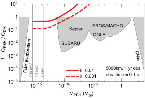 Figure 1
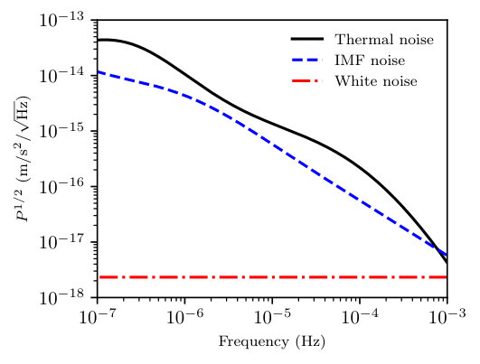 Figure 4
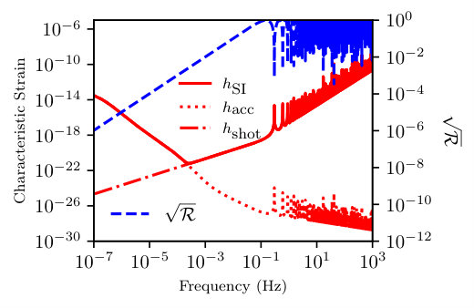 Figure 7
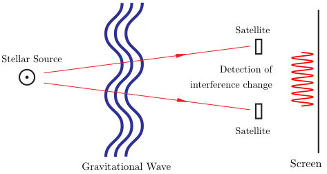 Figure 4
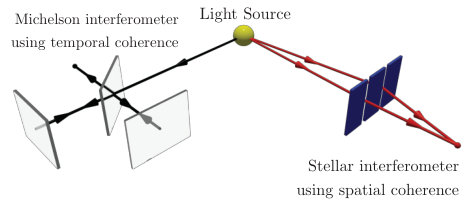 Figure 5
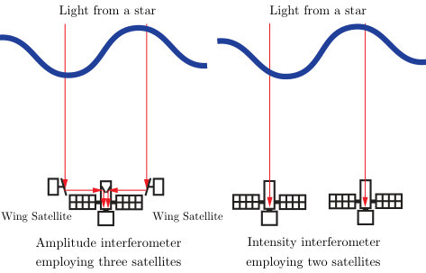 Figure 6
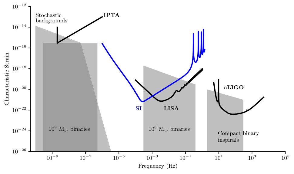 Figure 7
| Power spectral density | |
| Type of acceleration noise | ) |
| at Hz | |
| Spacecraft magnetic field effect | |
| Interplanetary magnetic field effect | |
| Combined magnetic field effect | |
| Radiation | |
| Radiometer | |
| Combined thermal effect | |
| Transformer thermal noise | |
| Cosmic ray momentum transfer | |
| Overall acceleration noise |
Peer Reviews
No public reviews on file for this paper yet. If you reviewed it on a platform where reviews are public (OpenReview, ICLR, NeurIPS, ICML), you can paste yours below so the community can read it here.
Videos
No videos yet. Explain this paper in a talk, walkthrough, or lecture? Add one.
Stellar Interferometry for Gravitational Waves
I. H. Park
K. -Y. Choi
J. Hwang
S. Jung
D. H. Kim
M. H. Kim
C. -H. Lee
K. H. Lee
S. H. Oh
M. -G. Park
S. C. Park
A. Pozanenko
C. D. Rho
N. Vedenkin
E. Won11footnotetext: Corresponding author.
Abstract
We propose a new method to detect gravitational waves, based on spatial coherence interferometry with stellar light, as opposed to the conventional temporal coherence interferometry with laser sources. The proposed method detects gravitational waves by using two coherent beams of light from a single distant star measured at separate space-based detectors with a long baseline. This method can be applied to either the amplitude or intensity interferometry. This experiment allows for the search of gravitational waves in the lower frequency range of to Hz. In this work, we present the detection sensitivity of the proposed stellar interferometer by taking the detector response and shot and acceleration noises into account. Furthermore, the proposed experimental setup is capable of searching for primordial black holes and studying the size of the target neutron star, which are also discussed in the paper.
1 Introduction
The discovery of gravitational waves (GWs) that originate from mergers of compact objects i.e. black holes (BHs) and neutron stars (NSs) [1] has successfully led us to a new era of physics, demonstrating Einstein’s theory of General Relativity. The recent detection of the GW170817 event by the LIGO and Virgo groups [2, 3], together with the successful electromagnetic (EM) follow-up observations by more than 70 observatories, has opened a new opportunity to better understand the makings of the universe. In addition, multi-wavelength observations will become increasingly important for GW astronomy, analogous to EM astronomy over the entire range of frequencies that has advanced over the preceding decades.
Multi-wavelength GW observation is foreseen from various detection methods. The most successful GW detectors, at present, are ground-based laser interferometers, i.e. LIGO [4, 5], Virgo [6], and KAGRA [7], while space-based laser interferometers such as LISA [8], DECIGO [9], and BBO [10] are expected to launch in the late 2020s or later. The ground interferometers are sensitive to GWs of around 100 Hz that are known to be driven by compact binaries, supernovae, and pulsars whereas space-based interferometers can detect GWs ranging from 1 Hz to Hz with the origin of resolvable supermassive blackhole (SMBH) binaries in the scale of [11] (Appendix A).
Interferometry, currently, is the most widely used method in detecting GWs that uses coherence of light, a measure of correlation between the phases at temporally or spatially different points on a wave. Laser based interferometers for GW detection such as LIGO and LISA are temporal coherence experiments, known as Michelson interferometer. These experiments take advantage of a significantly long coherence time of lasers. Here, we propose a new method, a stellar interferometry for the detection of gravitational waves using spatial coherence interferometry, as denoted hereafter by SI (Stellar Interferometry for gravitational waves). Instead of using a laser as a source, this method will use stellar light as the probe of space-time disturbance caused by gravitational waves. This method focusses on detecting low-frequency band GWs associated with SMBHs. The proposed SI can observe GW frequency range of Hz to Hz, corresponding to SMBH binaries of mass between and . This would complement the lower parameter space of LISA in the study of GWs using a completely different method [12, 13, 14, 15].
Furthermore, SI can be used as a testbed for other interesting physics. These include placing a better constraint on the size of the target neutron star and searching for the evidence of primordial black holes as a dark matter candidate. See Appendix A for more detail.
2 Model
The proposed SI will operate using a stellar source for its spatial coherence experiment, while LIGO and other similar observatories use lasers as their light source for temporal coherence. Basic principles and differences between spatial and temporal coherence interferometry are illustrated in Fig. 1. Stellar interferometry, for the purpose of studying stars, was first suggested in the 19th century by Hippolyte Fizeau [16]. He noted that the diameter of an extended disk could be determined interferometrically through the measurement of the baseline length at which the fringe contrast drops to zero. This concept was first exploited by Albert A. Michelson and Francis G. Pease [17]. In 1919, Michelson successfully determined the angular size of six supergiant stars to milliarcsec scale, among which was Orionis (Betelgeuse), measured at 0.047 arcsec. Note that for a single star, interference disappears when where is the distance between the two slits, is the wavelength of the incident EM wave, and is the angular diameter of the star [18].
For SI, we apply a similar methodology to detect gravitational waves in space. The most fundamental concept of SI is depicted in Fig. 2. While the experimental setup for a Michelson stellar interferometer and SI are identical, SI will monitor changes in interference patterns resulting from disturbances in space caused by gravitational waves.
SI can be best designed to be carried out in space, as shown in Fig. 3. A straightforward configuration is a constellation of three satellites (Fig. 3 left). A host satellite and two wing satellites, each equipped with a telescope for capturing stellar light from a stellar source. The two wing satellites will serve as a Michelson stellar interferometer by reflecting star light to a host satellite. The host satellite can collect and combine the reflected coherent lights and the interferometer will look for changes corresponding to gravitational waves in the resultant interference patterns.
As an alternative, a two-satellite system configuration is also viable, as shown in Fig. 3 right. This tandem configuration uses intensity (electrical) interferometry, pioneered by Hanbury Brown and Twiss [19, 20, 21], instead of amplitude (optical) interferometry. The intensity interferometer is more advantageous in space-based, long baseline experiments due to relatively simpler deployment and maneuvering of satellites. The two detectors would collect data with order picosecond time resolution. All of the data obtained from each of the detectors are stored that can be analysed offline to measure the cross-correlation of the intensity fluctuations (second order spatial correlation of electric fields) of the stellar light. The data from the two detectors with time stamps can be matched to find a pair of two signals that have a mutual coherence. This is a fundamental characteristic of intensity interferometry with long baseline, a great advantage over classical techniques involving real-time cross correlation. Real-time cross correlation keeps only the final product of the correlation and loses the original data from each detector, forbidding any further analysis of raw data. Moreover, this method removes the need for real-time controlling of the satellites with extreme accuracy and there is no physical connection between the two detectors.
In both cases, a drag-free system with a test mass is required. A summary of the acceleration noise and detailed description of the noise computation can be found in Section 3 and Appendix B, respectively.
The ideal orbit of the satellites can be determined depending on the chosen stellar source and the amount of reduction in noise. Some of the candidates would be the L2 (Lagrange point 2) orbit for the Sun-Earth system or a heliocentric orbit, both of which can be adopted with either the intensity or the amplitude interferometry. With minimal gravitational perturbation, long lifetime of spacecrafts, low temperature, and low background environments, the L2 orbit of the Sun-Earth system could be preferred for SI. Since the orbital plane around the L2 point can be chosen in any orientation, the position of the stellar source should not be problematic for the SI experiment. Furthermore, the SI experiment requires relatively light-weight satellites without a need for high power laser devices. Such aspects would reduce related noises as well as the cost and time required for the realization of the experiment.
3 SI Sensitivity
3.1 Stellar source and response function
The distance between the two slits, i.e. satellites, is an important parameter for GW detection and the detection sensitivity of SI. The separation between two satellites depends on the spatial coherence length of a given star and thereby its distance from the satellites and the size of the star. For the visible light of 550 nm, a few promising candidates include SMC AB8 (12.83 mag, 197,000 Ly distance, km) and the Crab Pulsar (16.5 mag, 6,523 Ly distance, km). A very small area of the Sun can also serve as a stellar source with magnitude and 0.1 milliarcsec of parallax that corresponds to area of the Sun’s surface, granting km. For the calculation of the sensitivity, we chose a half of the actual computed (maximum) as our , which would translate to a fringe visibility of approximately 0.6 in coherence experiments. Note that the is not necessarily the most optimal choice. For given parameters of a stellar interferometer with and the magnitude of a star, we need to calculate the path length difference perturbed by a GW in terms of strain . This dimensionless quantity gives a fractional change in the path length of a photon emitted from a star, as defined by where is the characteristic length that corresponds to half the target wavelength of GW () in the case of SI. The response of the detector should be considered in terms of a response function that reflects the geometrical configuration of the detector with respect to the GW propagation. This response degrades the sensitivity of GW signal () hence this factor is divided from the strain noise () as given by . A detailed calculation of the response function is discussed in Appendix B. For the calculation of the sensitivity, we initially assumed orthogonal GW propagation direction with respect to our line of sight to obtain maximum sensitivity. Then, for the final estimation of the sensitivity, we took into account the change in the orientation due to orbital movements of the detector satellites.
3.2 Photon statistics and noise
The noise components arise from the detection process in many varieties and forms, that may sit on top of GW signals. The sensitivity of SI is determined primarily by two major sources of noise. One is shot noise due to the limitation of the luminosity of the target star as a light source. The other is acceleration noise that is instrument and/or experiment specific. Interferometric detectors are limited at high frequencies by the shot noise, which arises due to the randomness in the production of photons from their source. Shot noise can be calculated using the uncertainty principle: where is the reduced Planck constant. In terms of the uncertainty in the photon number () and displacement (), it can be shown that the minimum detectable change by a gravitational wave is given by and . Each photon from a source arrives at a receiver at random times but with an average rate that is proportional to the signal strength. For this type of phenomena, the number of events that occur in a given time interval varies statistically, following a Poisson distribution. For a stellar source with optical power , the average number of photons that arrive within is given by and the root-mean-square deviation becomes . Thus, a minimum detectable change from the shot noise can be written as
[TABLE]
Due to the orbital motion of the spacecraft and the relative position of a GW source with respect to the orbit, the maximum amplitude cannot be achieved. It is reduced by a factor of , when an average of interferometer response is taken with respect to the entire sky [22]. Furthermore, the separation between two satellites () may not be comparable to the wavelength of GW’s, hence the response is further impeded by an order of . There is a trade-off between and that a small means higher visibility but it also needs to be high enough to be comparable to for better sensitivity.
A star of apparent magnitude 8 yields optical power of W for R-band with m. Note that the available optical power for LISA is W. Finally, the minimum detectable change in SI can be computed using
[TABLE]
where is the integration time equivalent to . This equation includes our choice of , which implicitly contains the effect of having the visibility of 0.6. A full derivation of Eq. (3.2) can be found in Appendix B.
Another noise component, dominant in the lower frequency range, is the acceleration noise. This noise is associated with external forces and is produced from fluctuations of magnetic field, electric field, gravity, temperature, and pressure acting on the detector. For SI, the orbital plane of the satellites can specifically be chosen to be maintained perpendicular to the line of sight to the reference star. SI will have the light propagation paths perpendicular to the satellite orbital plane, and thus potential forces, i.e. drag forces. This means any associated acceleration noise, in the direction of the satellite motion, should not affect SI. In any case, an accurate force sensing system with a drag-free system consisting a test mass can measure these acceleration noise and estimate the effects of various forces, which will be important for distinguishing them from the effects of a true GW signal.
In this work, we separately consider three categories of acceleration noise acting on a test mass, namely, magnetic field, thermal, and other white noise. The test mass for the calculation of acceleration noise is made of Pt-Au alloy with a mass of 2.00 kg and a dimension of (4.64 cm)3, similar to the one used for the LISA pathfinder [23]. For the forces associated with magnetic fields, the two leading components acting on a test mass are magnetic field fluctuations due to the couplings between: 1. The fluctuation in the spacecraft (self-generated) magnetic field and the gradient of the spacecraft magnetic field, 2. the fluctuation in the interstellar magnetic field (IMF) and the gradient of the spacecraft magnetic field. The noise components are found to be , and at Hz, respectively. See Appendix B for detailed derivations. These noise components may be further reduced by using a modern state-of-the-art shielding with active cancellation, minimizing electronic parts of the detector and current loops, and choosing appropriate orbital geometry.
The thermal noise arises from the temperature difference between the walls of the housing that encases the test mass. For SI, the two main factors contributing towards the thermal noise are due to: 1. different radiation rates between the walls of the housing, 2. the residing gas molecules in the housing interacting with the test mass. The outgassing of the housing walls, on the other hand, should be negligible compared to the other two effects. In this work, we assume a stabilized and well-monitored environment with K, giving us the total thermal noise of at Hz. Refer to Appendix B for the full derivation.
The remaining noise for SI is white noise of which the two most dominant components are due to: in-phase transformers and collisions by cosmic-ray particles. The in-phase transformer noise is produced from the heating of the transformers placed in the drag-free system. On the other hand, the cosmic rays produce noise when they collide into the test mass, which the results have been calculated by other works. All in all, we find the contributions from the two noise components to be , and , respectively (see Appendix B).
3.3 Results
The overall acceleration noise is computed as at Hz. Each of the acceleration noise component represented as power spectral density is presented in Table 1 and shown in Fig. 4.
Figure 5 shows the sensitivity budget for SI with the shot noise, acceleration noise, and response function included. After taking into consideration all the factors, the final strain sensitivity of SI can be estimated as where S_{n}=\bigg{(}\frac{P_{\textrm{shot}}}{L^{2}_{c}}+\frac{P_{\textrm{acc}}}{(2\pi f)^{4}L^{2}_{c}}\bigg{)} \cdot\Big{(}\frac{1}{\mathcal{R}}\Big{)} is the strain noise power spectral density squared, and and are the power spectral densities for shot noise and acceleration noise, respectively. The power spectral density, is given by from Eq. (3.1) and is estimated as shown above. Here, the factor includes the effect of the quadratic sum of two detector noises, variations of gravitational wave directions with respect to our line of sight due to the orbital motion of the spacecrafts, and the 5 of the signal to noise ratio. Choosing 550 nm visible light from the Crab Pulsar as the stellar source, and 1,000,000 km as the displacement between the two satellites, we calculate the GW detection sensitivity for SI in red in terms of characteristic strain and GW frequency as shown in Fig. 5.
According to Eq. (3.2), the sensitivity improves when using the starlight with shorter wavelengths. From the relation of , however, longer source wavelengths should always be preferred to achieve larger when using the same stellar source with equal angular size. Since X-rays have relatively shorter wavelengths, a smaller source and/or higher power is required to have the sensitivities comparable to those of UV/optical. Low-mass X-ray binaries (LMXBs) can be one of the best X-ray source candidates for SI because of their relatively high power and the small size of neutron stars. For X-rays of 2 keV energy, using a typical neutron star radius of 13 km and a distance of 3.6 kpc to 4U 1608-522, the expected satellite separation is of the order 3,200 km. A sensitivity curve for 4U 1608-522 is presented in Fig. 5 in blue along with the Crab pulsar in red. Here, we assume 10% detector efficiency during the computation of the X-ray results. Furthermore, using X-rays can also lead to other interesting physics studies such as searching for primordial black holes as dark matter (DM) candidates and studying macroscopic properties of the target neutron star. For more details, please see Appendix A.
4 Conclusion
We propose, for the first time, stellar interferometry for the detection of gravitational waves with spatial coherence of starlight. We calculate the GW detection sensitivity for both stellar sources by considering the shot and acceleration noise components and the response function for the stellar interferometer. From Fig. 5, we obtain the minimum characteristic strain of at Hz for the Crab pulsar, where the acceleration noise is divided into three components, namely magnetic, thermal, and white, which in total gives at Hz. Also, the shot noise is found to be . As well as optical stellar sources, X-rays emitted from LMXBs can be used as the probes for gravitational waves. For 4U 1608-522, we obtain the minimum characteristic strain of at Hz, where the acceleration (shot) noise is (). We anticipate that this new method will benefit the field, producing complementary results to further our knowledge on gravitational waves.
Appendix A Other applications
A.1 Gravitational wave sources of low frequency bands
Supermassive black holes (SMBHs) are expected to exist at the center of almost all galaxies and have a typical mass of around . The observed correlations between the mass of SMBHs and the velocity dispersion, mid-infrared luminosity, and mass of stellar bulges inside host galaxies imply the importance of SMBHs for studying the formation and evolution of galaxies. Recent observations of distant quasars indicate that SMBHs have existed from the early stages of the universe, 690 Myr after the Big Bang [27]. Although the formation and evolution of SMBHs are still unclear, it is believed that the SMBHs evolved from initial seeds with a mass of around at a redshift of . These initial seeds may have formed from the remnants of Population III stars or directly from the collapse of dense gas clouds. In CDM cosmology, dark matter halos and galaxies are formed hierarchically by the merger of smaller structures. When two galaxies merge, the SMBHs at the center of each galaxy sink into the central region of the merged galaxy by dynamical friction and form a binary system. An SMBH binary then spirals in and eventually merges as it loses gravitational energy in the form of GWs that are detectable at Earth. During an inspiral of SMBH binaries, the frequency of GW increases with time, making characteristic tracks on the plane of the frequency-characteristic strain. With a mass of , the frequency should span from Hz to Hz with a characteristic strain amplitude of for a few months. The proposed stellar interferometer can observe SMBH binaries with their total mass spanning between and by focusing on the GW frequency range of Hz to Hz. This fills yet to be considered parameter space in the study of gravitational waves, i.e. the gap between the range of LISA ( Hz) and the one of PTA ( Hz). The measurement of the amplitude and spectrum of GWs in the frequency range between Hz to Hz will enable us to better understand the formation and evolution of SMBHs, as well as their link to galaxy evolution. Another target GW source of SI frequency band is extreme mass-ratio-inspirals (EMRIs) with a mass ratio greater than : 1 between the binary pairs. The large mass difference between two objects allows us to observe the effects of gravity in the strong-field limit, which is difficult to achieve with stellar-mass binaries. EMRIs [28, 29] are binary systems containing a massive black hole that eventually merges with its smaller companion such as a white dwarf, neutron star, stellar mass black hole or a giant star with a helium core. The final stages of EMRI mergers produce GWs between Hz to Hz. LISA is most sensitive in this frequency band, while the marginal range of the gradually inspiraling phase can be covered by SI.
A.2 Probing primordial black hole (PBH) DM with LMXB lensing parallax
The PBH in the lightest mass window of can theoretically account for the full DM abundance. The only reliable lensing method that can probe this window is lensing parallax of a compact source such as gamma-ray bursts (GRBs) [30, 31] and microlensing of LMXBs [32]. SI with long baseline is potentially an ideal laboratory for the detection of lensing parallax. In this subsection, we provide a brief estimation of LMXB lensing parallax using an SI setup. The Einstein radius of the lightest PBH is given by km for at a Gpc distance. This is indeed shorter than the SI baseline of 5,000 km so one of the detectors may measure more lensing magnified LMXB than the other, i.e. a lensing parallax. The brightness resolution is then a key detector parameter. We will assume a fractional resolution obtained from 100 ms stacking to be (reasonable) or 0.001 (optimistic). With a yearlong tracking of a single LMXB, SI can essentially cover many patches of the Einstein angle; it is equivalent to observing the same large number of LMXBs. The large number can compensate for the small lensing optical depth of a nearby LMXB ( 6 kpc). The source of thermonuclear LMXBs is thought to be the neutron star with a radius of 10 km, which indeed appears to be smaller than the Einstein angle, hence allowing efficient lensing. The X-ray spectrum of LMXBs typically peaks at keV, which is high enough to see PBHs more massive than . The estimated sensitivity on the PBH DM abundance is shown in Fig. 6. With the aforementioned SI design, a large part of the unconstrained PBH mass window can indeed be probed using SI. The most crucial capability that can be further improved is the brightness resolution, e.g. via larger detector area and/or higher sampling frequency.
A.3 Probing macroscopic properties of neutron stars
The two X-ray detectors of SI can be used as an HBT intensity interferometer [19, 20, 21], which can measure the radius of a target neutron star. Each detector can be used as an X-ray spectrometer that can measure the mass and the radius of the neutron star simultaneously. Macroscopic properties of neutron stars, such as masses, radii, and temperatures, have been studied using X-ray spectroscopy during quiescence of LMXBs [33]. Typical temperatures of neutron stars in the observed LMXBs are in the range of keV [34, 33]. With two X-ray detectors of SI that are sensitive to keV photons, one can measure the temperature of the target neutron star. In combination with the total measured flux, the mass and radius of the neutron star can be estimated by assuming blackbody radiation and the Eddington flux [33]. This information can provide constraints on the neutron star equation of state to determine the inner structure of neutron stars. Neutron star equation of state is still unknown mainly due to the uncertainties in the high-density behavior of dense hadronic matter. With the help of recent measurement of tidal deformability of neutron stars from the gravitational wave event GW170817 [2, 3], very hard equations of state have been ruled out. On the other hand, observations of 2 neutron stars in neutron star - white dwarf binaries ruled out very soft equations of state [35, 36, 37]. Recent observations by the Neutron Star Interior Composition Explorer also put new constraints on the radii of neutron stars [38, 39]. Even though these results narrowed down the region of allowed equations of state in the parametric space of neutron star mass and radius, the allowed region is still quite large. Therefore, simultaneous measurements of mass and radius of a neutron star by SI will produce important results to better understand the physics of high dense hadronic matter.
A.4 Relic stochastic background gravitational waves
The relic stochastic background of gravitational waves (RSBGW) was predicted from zero quantum oscillations due to strong gravitational fields of the early universe [40, 41]. The primary spectrum of RSBGW depends on the parameters and models of the expanding universe. The current spectrum is a result of the evolution of the Universe, in a particular of re-processing the primary spectrum at stages dominated by radiation and matter [42, 43]. Indeed, the spectrum can be described by a power law. The primary spectrum is intact at frequencies below the Hubble frequency of Hz, and thus, the normalization of an observable spectrum can be obtained from the current observations of the CMB.
The sensitivity of the SI at Hz is marginally comparable with the currently assumed amplitude of for RSBGW. The spectrum registering at these frequencies is composed at least from a binary stochastic background and RSBGW. It is a stochastic signal arising from un-resolvable signals of numerous binary systems. The binary background can be estimated much better than the RSBGW. Hence, we will have a unique opportunity to directly estimating the RSBGW amplitude at the low frequencies. Estimates of upper limits of the stochastic gravitational-wave background as well as the binary stochastic background have already been obtained by LIGO/Virgo observations at high frequencies [44, 45].
Appendix B Computing SI Sensitivity
B.1 Full Derivation of characteristic strain
This derivation follows closely the procedures shown in [46], and was altered to conform with the experimental setup of SI. The average power of starlight during the observation time is given by where is the average number of photons arriving at the detector within , is the angular frequency of the EM wave we will be observing. Using Poisson distribution and , we get:
[TABLE]
For the GW propagating in the -direction, the space-time interval is given by
[TABLE]
where we used “+ polarization” only for simplicity given by . For the starlight travelling towards the satellites in the -axis, we get
[TABLE]
Also, the two signals for the two satellites separated by in the -axis (the satellite (1) is located at and (2) is at ), are given respectively by,
[TABLE]
where and () are the amplitude and frequency (wave number) of the gravitational wave. Let us assume photons emitted from our star by a gravitational wave intersecting the photon propagation path. The photon is affected by the gravitational wave from a time and travels a distance at a time . Using Eq. (B.3), the distance becomes:
[TABLE]
To first order, hence at we can re-writte as:
[TABLE]
Since we observe the photon at a given time , now setting and using Eq. (B.4), we get the time
[TABLE]
Using sinc function and at leading order, we can rewrite Eq. (B.7) for the first satellite as:
[TABLE]
The last term in Eq. (B.8) is the phase change due to gravitational wave for the first satellite, denoted as . Similarly, for the second satellite located at , we follow the same procedure with the second equation of Eq. (B.4). Hence, we simply remove from Eq. (B.8) and get:
[TABLE]
Therefore, the phase difference of two lights measured at the satellites (1) and (2)
[TABLE]
Here we define the response function as
[TABLE]
up to the time-dependent term. For the low frequencies of GW, the response function is reduced by the second term representing the ratio between the spacing between the two satellites and the wavelength of the gravitational wave being detected. On the other hand, for the high frequencies, the response function oscillates. Fig. 7 shows the response function for the Crab Pulsar observed with 550 nm visible light. Here, we specifically picked the observation time so that . In the case of the distance from the star to the satellites being much larger than , the effects of the gravitational waves corresponding to the integer multiples of will be cancelled out. Now, for the total signal power [46], we have
[TABLE]
and the variation in power due to a GW is
[TABLE]
where we used for the simplest case, and the phase is a parameter that the experimenter can adjust, hence we can choose the best working point. The variation in power due to the shot noise is
[TABLE]
Finally, we obtain the signal-to-noise ratio:
[TABLE]
For the characteristic length , and in the limit of , and , we obtain
[TABLE]
Combining above with the signal-to-noise ratio equation written in terms of the strain sensitivity [46, 47],
[TABLE]
we find that
[TABLE]
Hence, in Fig. 5, we plot the characteristic strain defined as [24]:
[TABLE]
where , which indeed is the same as what we obtained in Eq. (3.2) from the uncertainty principle. In Fig. 7, are shown again with the sensitivity of SI only with the shot noise or the acceleration noise.
B.2 Magnetic field effect
The magnetic fields affecting the SI are due to “spacecraft” () and interplanetary (). The amount of force, due to these magnetic fields, experienced by the test mass is given by , where is the volume of the test mass, is its magnetic susceptibility, and is the vacuum permeability. Since the gradient of is very small (0.5 nT/10,000 km), terms are ignored. Here, we assume a Pt-Au alloy test mass of 2 kg with and test mass density . For , data from reference [48] have been used. Hence, the power spectral density squared on the magnetic field effects at Hz is
[TABLE]
where we assume and to be and , respectively. From this equation, .
B.3 Thermal effect
We have considered three effects caused by pressure changes within the test mass chamber due to temperature fluctuations, which are due to outgassing and radiation from the chamber walls, and any residing gas within the chamber. Firstly, the outgassing rate decreases exponentially with temperature. Hence, at 50 K, which is the environment we are considering for this experiment, the outgassing rate becomes negligible. Secondly, the noise from the radiation effect arises when the pressure is produced by the difference in temperature between opposite housing walls, i.e. , where is the Stefan-Boltzmann constant. Therefore, the change in pressure is given by
[TABLE]
At Hz range, we expect to be able to control to 570 K. Hence, the acceleration caused by the radiation effect becomes
[TABLE]
where is the area of a test mass wall and is the mass of the test mass. Lastly, the thermal effect from residual (ideal) gas that collide with the test mass should produce acceleration equal to
[TABLE]
where is the number of moles and is the Boltzmann constant. Here, is the pressure within the housing, that when exposed to the L2 space environment could be assumed as Pa. All in all, the corresponding thermal acceleration noise at Hz is
[TABLE]
where we assume K and is the frequency dependent term after the Fourier transformation of the accelerations above. The thermal component shown in Fig. 4 is obtained by convolving the solar flux [49] with a transfer function of solar energy from solar panel to detector on board the spacecraft.
B.4 Other noise
There are two other dominant noise components we consider for this work. First is due to the temperature rise of the in-phase transformers in the drag free system. Assuming we will use a similar drag free system as LISA, we adopt their value of [50]. Second is due to cosmic-ray particles colliding with the test mass, transferring their momenta. This can be estimated as
[TABLE]
Here, is the average momentum of each cosmic-ray particle, is the number of particles per time that fully transfer their momenta. Considering the incident angle (0.9 sr) and the test mass surface area () long with the known cosmic-ray flux at 1 GeV, the corresponding cosmic-ray noise is .
Acknowledgments
We are grateful to Antoine Labeyrie for his suggestion of Crab Pulsar as a light source for stellar interferometery. We would also like to thank Sunkee Kim, Hyungwon Lee, Jongmann Yang, Soomin Jeong, Chanyeol Kim, Chunglee Kim, Jiwoo Nam, Jean Schneider, Denis Mourard, and Rijuparna Chakraborty for fruitful discussions on noises and light sources. We acknowledge the support from the National Research Foundation (NRF) of Korea: I.H.P. NRF-2017K1A4A3015188, NRF-2021R1A2B5B03002645, and NRF-2019H1D3A2A02060090; K.-Y.C. NRF-2019R1A2B5B010701 81; J.H. NRF-2021R1A2C101109811; S.J. NRF-2019R1 C1C1010050; D.H.K. NRF-2018R1D1 A1B07051276; C.H.L. NRF-2016R1A5A1013277 and NRF-2018R1D 1A1B07048599; S.H.O. NRF-2019R1A2C2006787; S.C.P. NRF-2021R1A4A20 01897 and NRF-2019R1A2C1089334; C.D.R. NRF-2018R1A6A1A06024977; E.W. NRF-2017 R1A2B3001968. A.P. acknowledges the support from RSCF grant 18-12-00378.
The reference list from the paper itself. Each links out to its DOI / PubMed record.
- 1[1] B. P. Abbott et al. , Observation of Gravitational Waves from a Binary Black Hole Merger , Phys. Rev. Lett 116 , 061102 (2016).
- 2[2] B. P. Abbott et al. , Multi-messenger Observations of a Binary Neutron Star Merger , Astrophys. J. Lett. 848 , L 12 (2017).
- 3[3] B. P. Abbott et al. , Observation of Gravitational Waves from a Binary Neutron Star Inspiral , Phys. Rev. Lett. 119 , 161101 (2017).
- 4[4] A. Abramovici et al. , LIGO: The Laser Interferometer Gravitational-Wave Observatory , Science 256 , 325-333 (1992).
- 5[5] G. M. Harry et al. , Advanced LIGO: the next generation of gravitational wave detectors , Classical Quantum Gravity 27 , 08406 (2010).
- 6[6] F. Acernese et al. , Advanced Virgo: a second-generation interferometric gravitational wave detector , Classical Quantum Gravity 32 , 024001 (2014).
- 7[7] T. Akutsu et al. , KAGRA: 2.5 generation interferometric gravitational wave detector , Nature Astronomy 3 , 35 (2019).
- 8[8] K. Danzmann, LISA Laser Interferometer Space Antenna–A proposal in response to the ESA call for L 3 mission concepts , Albert Einstein Inst. Hanover, Leibniz Univ. Hanover, Max Planck Inst. Gravitational Phys., Hannover, Germany, Tech. Rep (2017).