Future Prospects for Constraining Nuclear Matter Parameters with Gravitational Waves
Zack Carson, Andrew W. Steiner, Kent Yagi

TL;DR
This paper explores how future gravitational wave observations from neutron star mergers can better constrain nuclear matter parameters by analyzing correlations between tidal deformabilities and nuclear physics, considering multiple events and systematic errors.
Contribution
It extends previous correlation analyses to varying chirp masses and proposes methods to improve nuclear parameter constraints using multiple detections and multidimensional correlations.
Findings
Future GW observations can improve nuclear parameter bounds by ~30%.
Systematic errors mainly stem from uncertainties in the equation of state.
Multidimensional correlations can reduce systematic errors.
Abstract
The gravitational wave emission from the merging binary neutron star system GW170817 arrived full of tidal information which can be used to probe the fundamental ultra-dense nuclear physics residing in these stars. In previous work, we used two-dimensional correlations between nuclear matter parameters and tidal deformabilities of neutron stars applying specifically to GW170817 to derive constraints on the former. Here, we extend this analysis by finding similar correlations for varying chirp masses, the dominant determining factor in the frequency evolution of the inspiral, such that one can apply the same method to future detections. We estimate how accurately one can measure nuclear parameters with future gravitational wave interferometers and show how such measurements can be improved by combining multiple events. We find that bounds on the nuclear parameters with future…
Click any figure to enlarge with its caption.
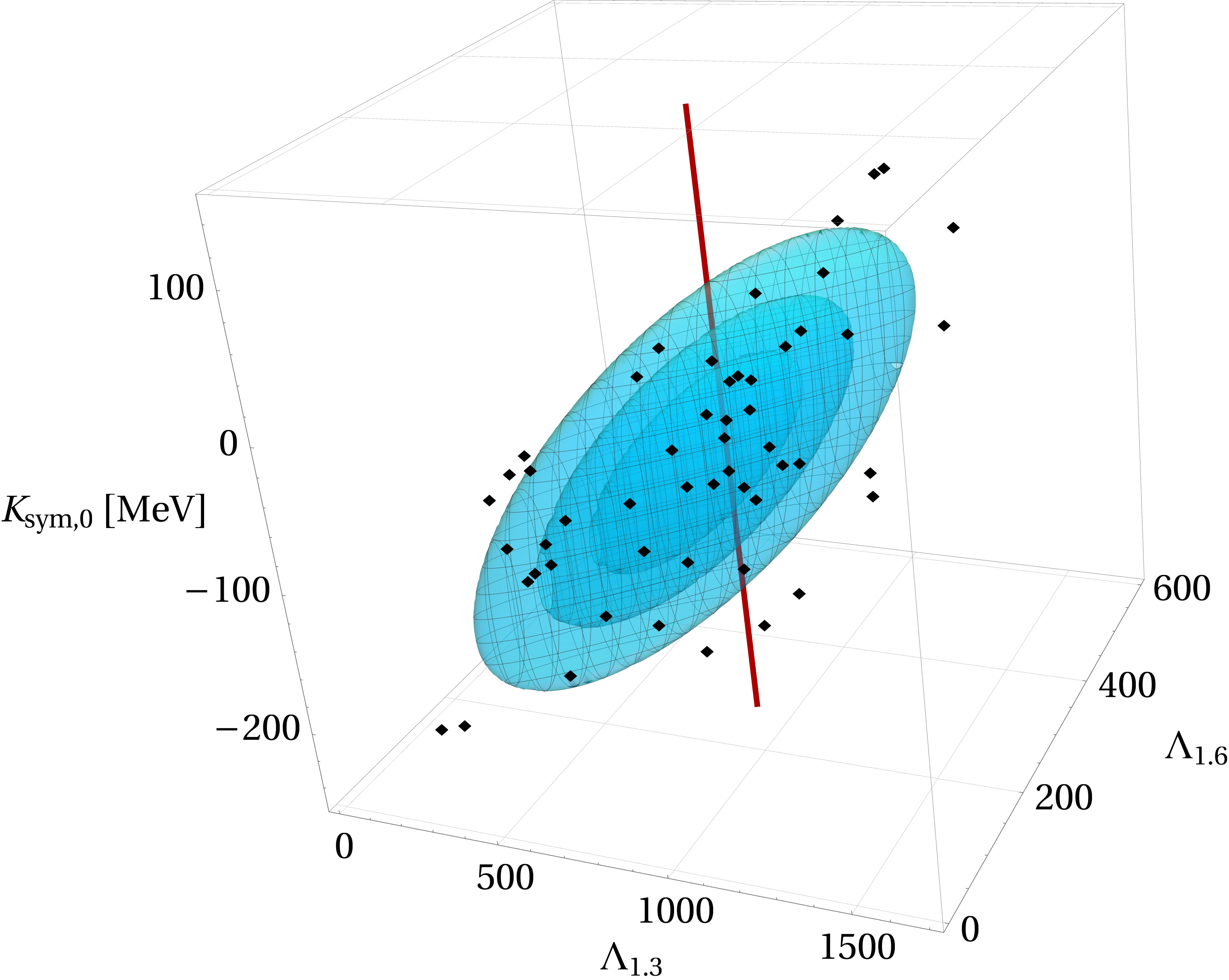 Figure 1
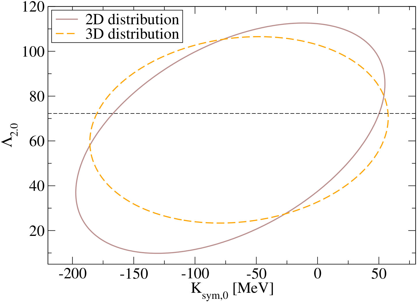 Figure 2
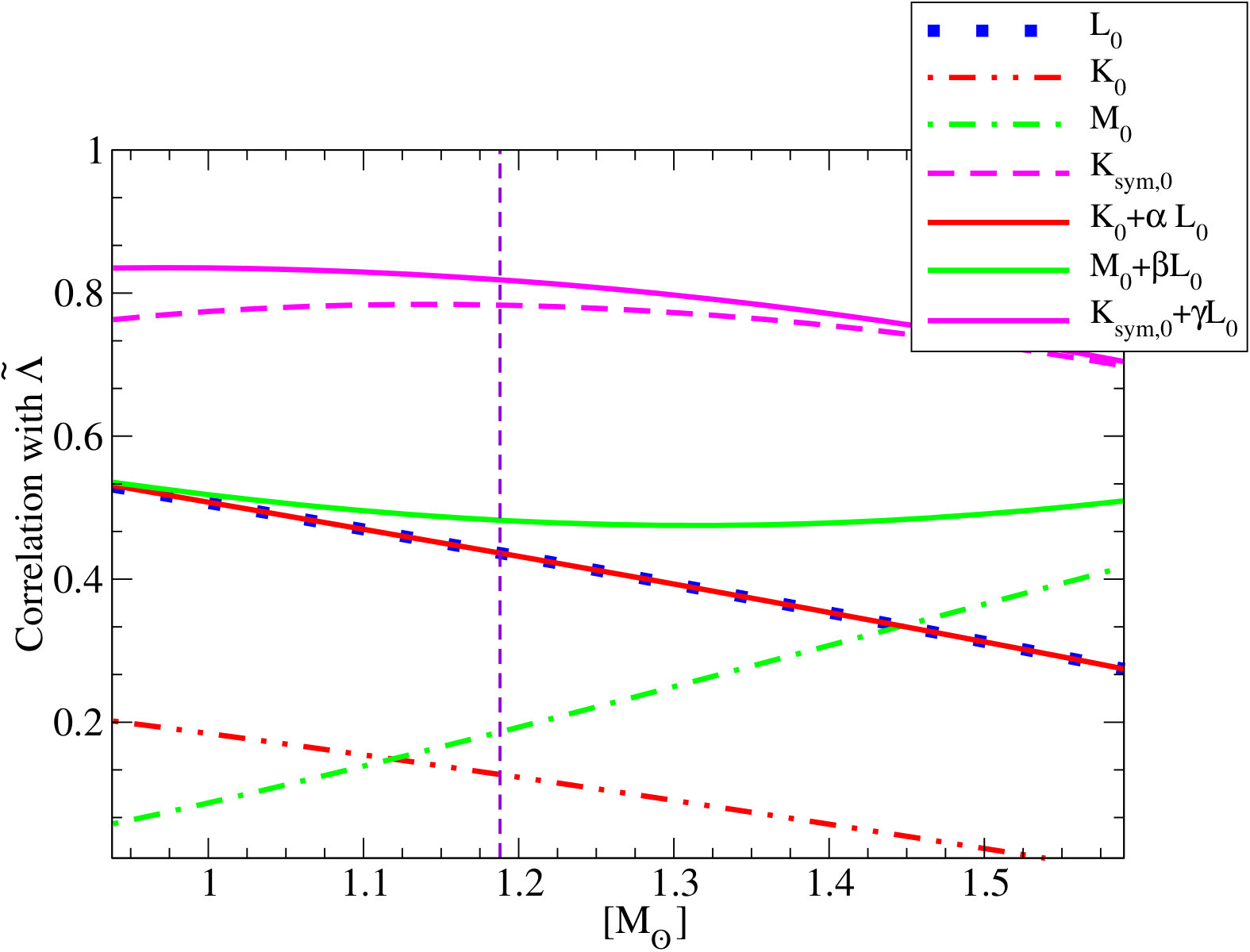 Figure 3
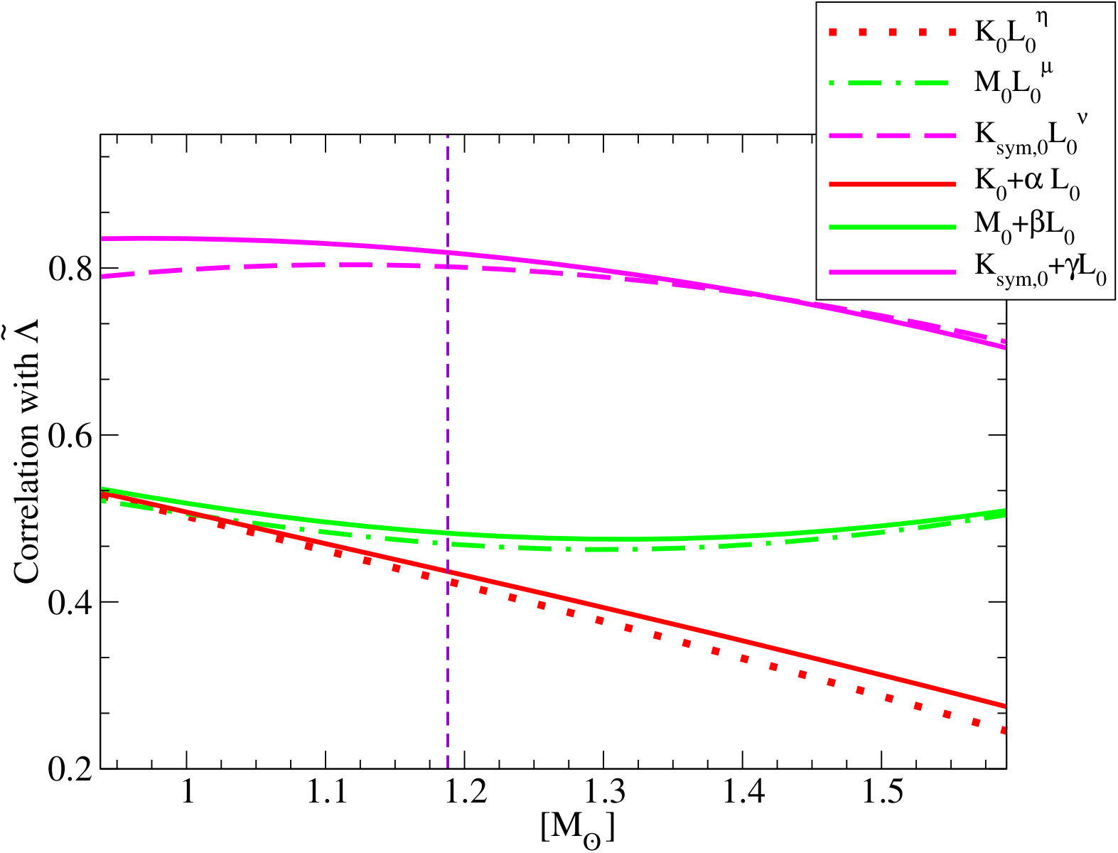 Figure 4
 Figure 5
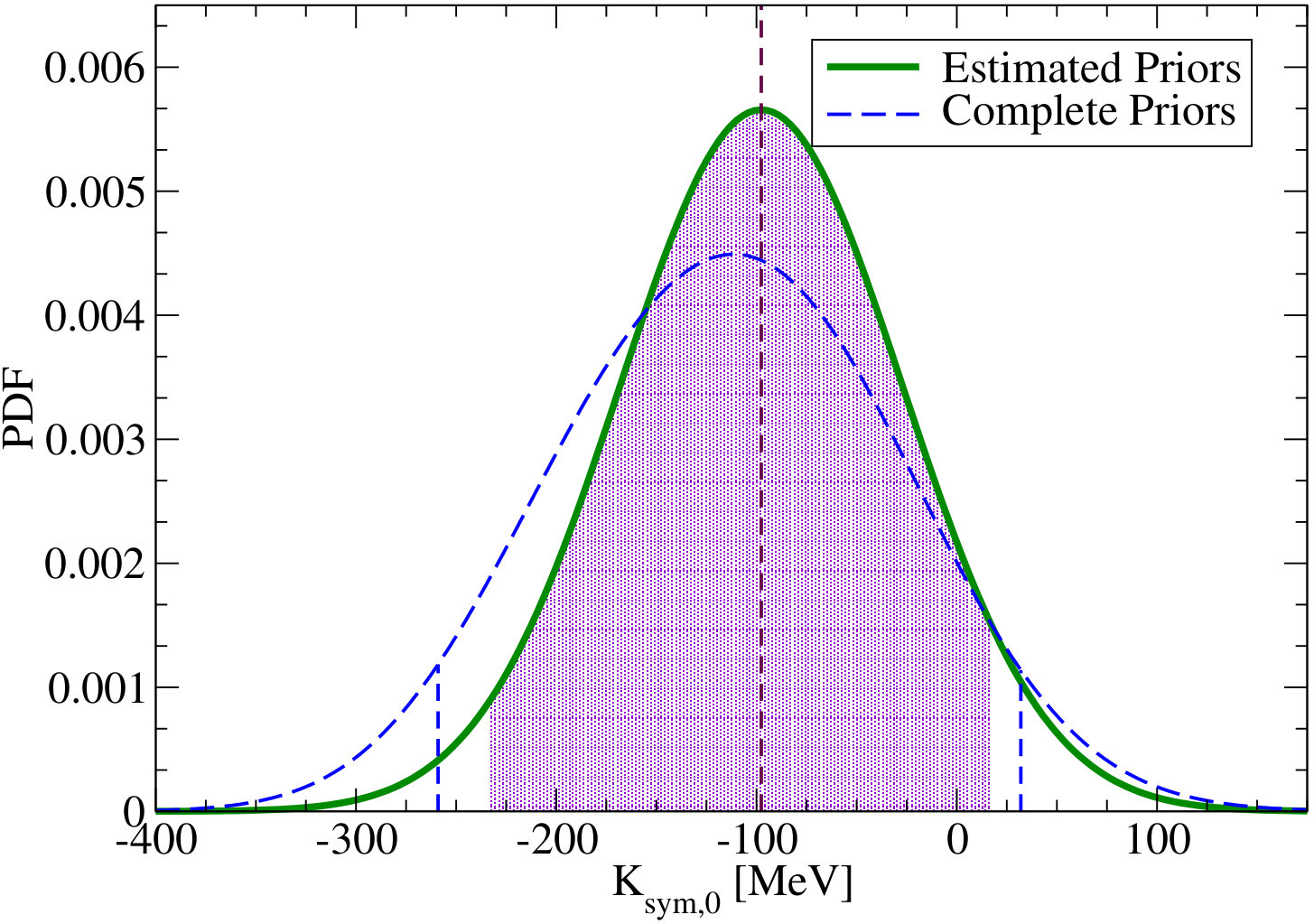 Figure 6
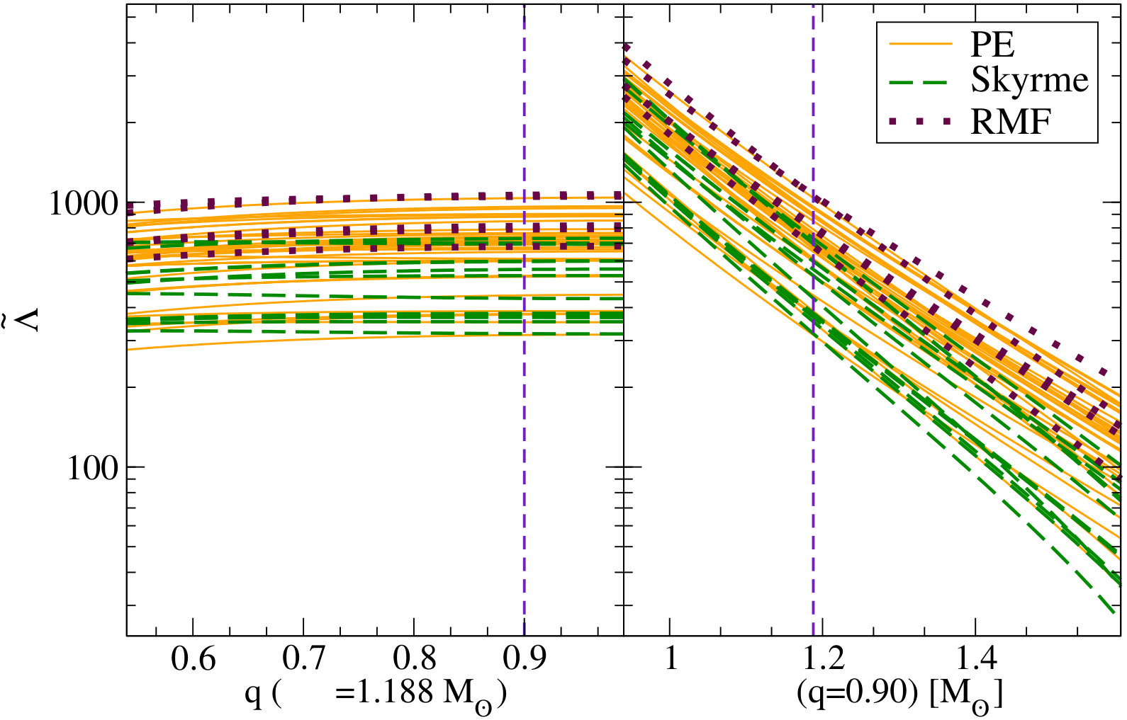 Figure 7
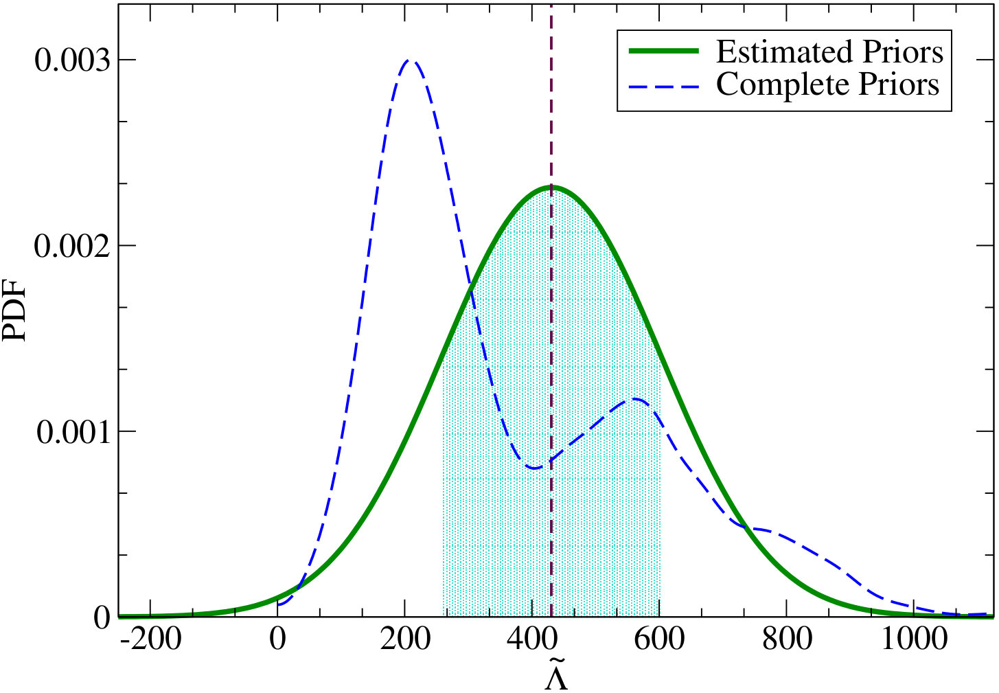 Figure 8
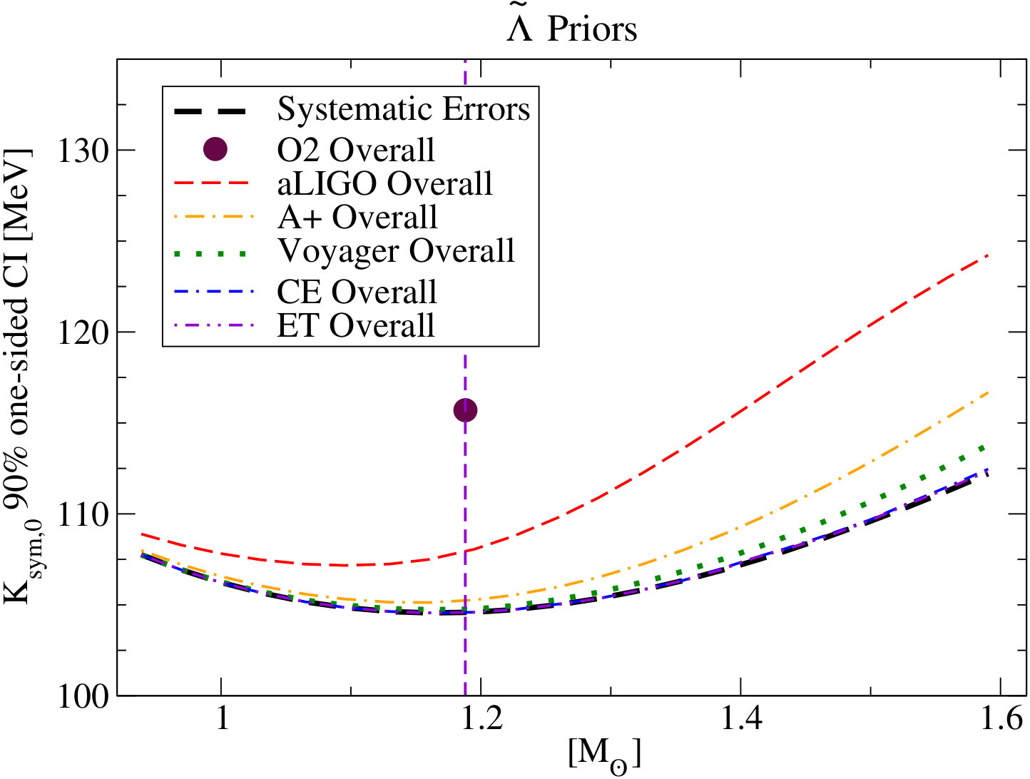 Figure 9
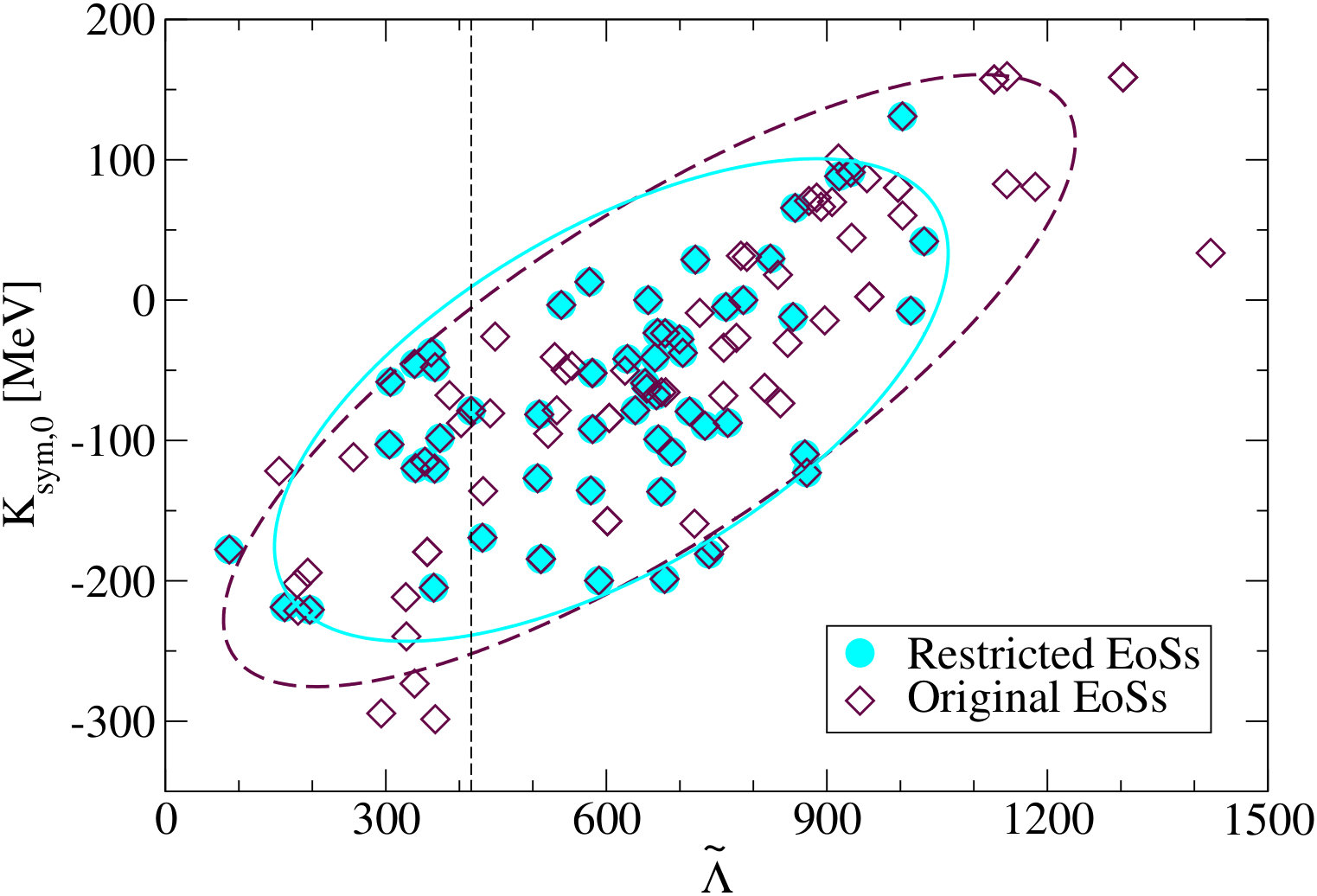 Figure 10
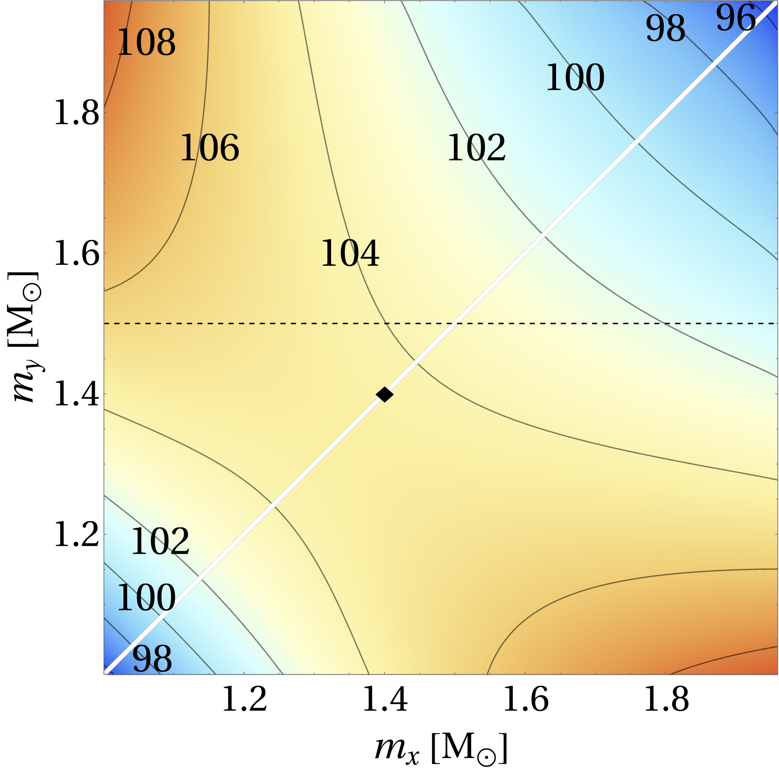 Figure 11
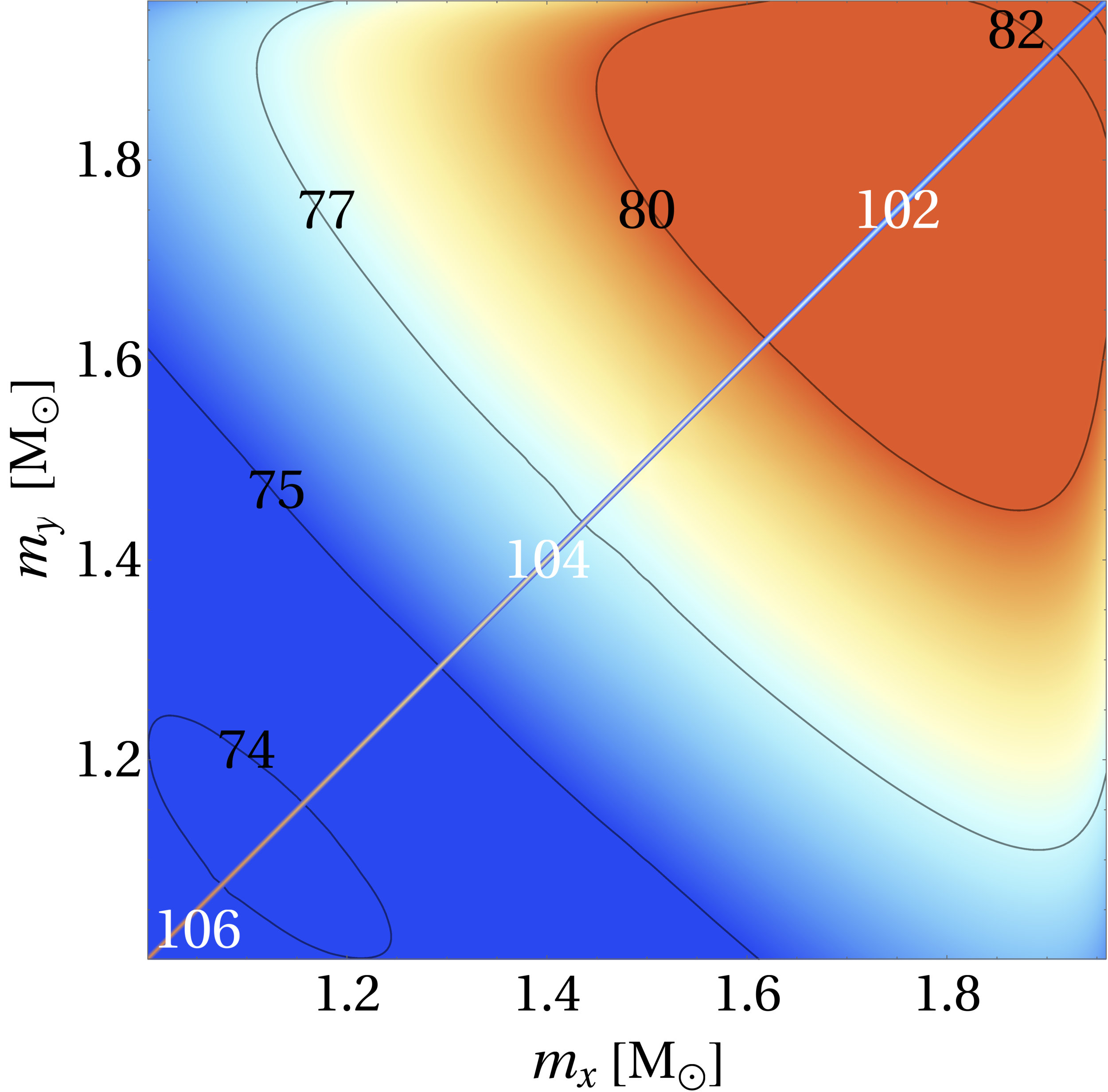 Figure 12
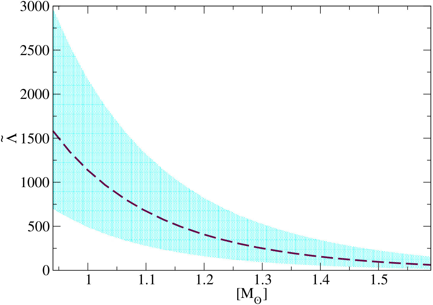 Figure 13
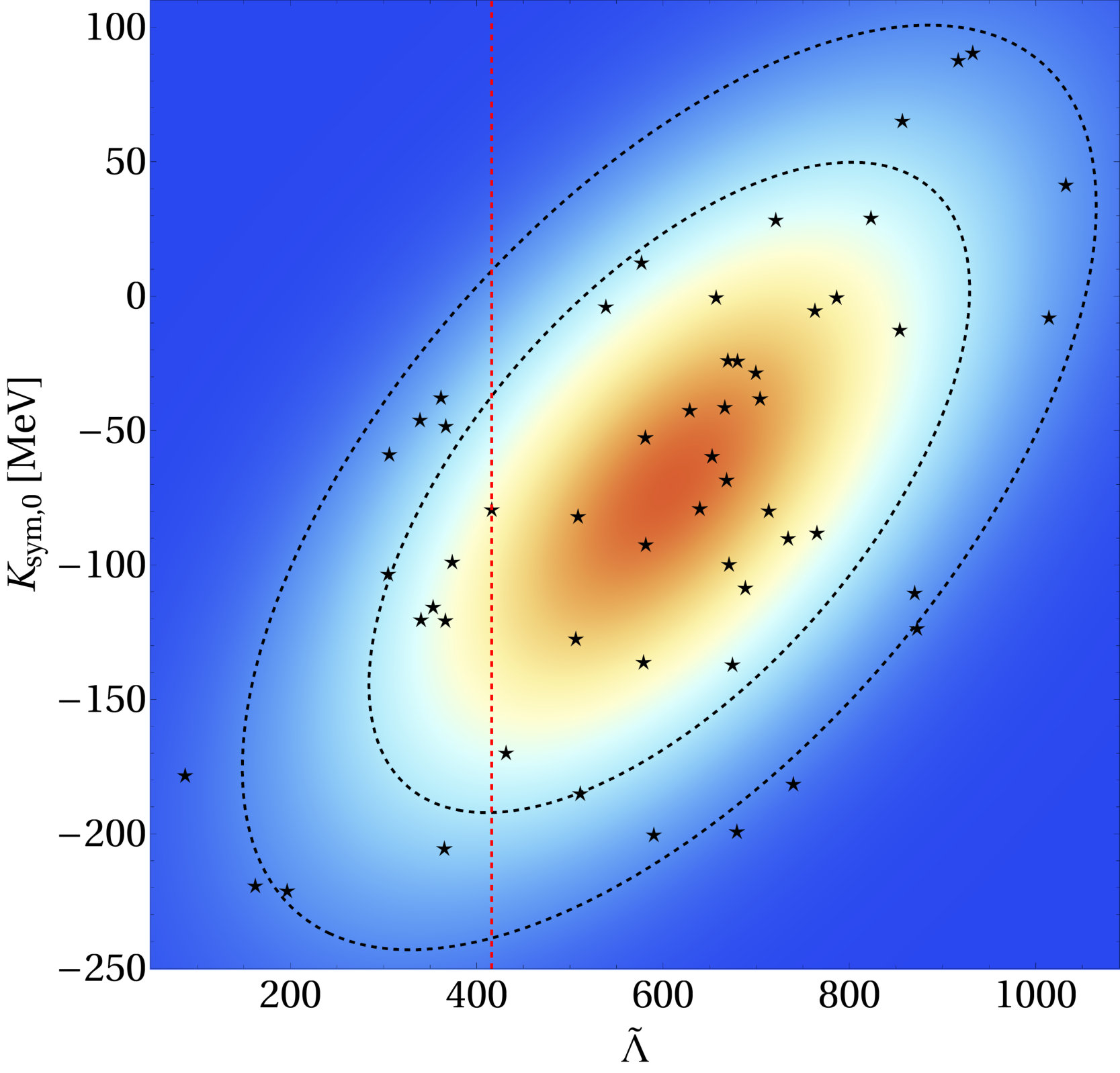 Figure 14
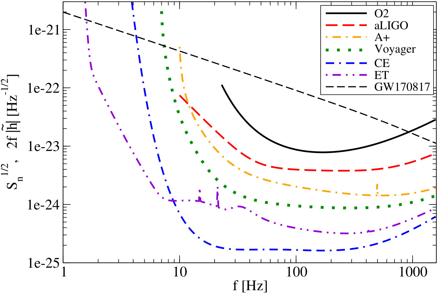 Figure 15
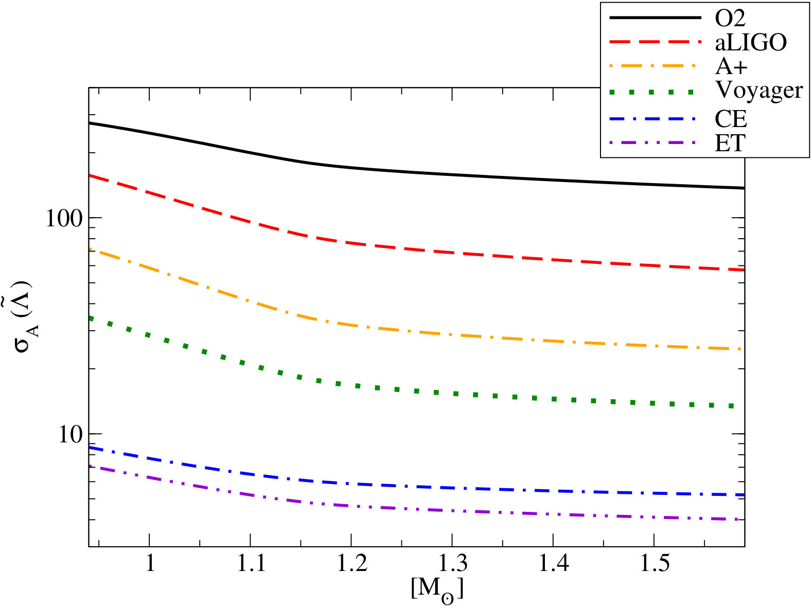 Figure 16
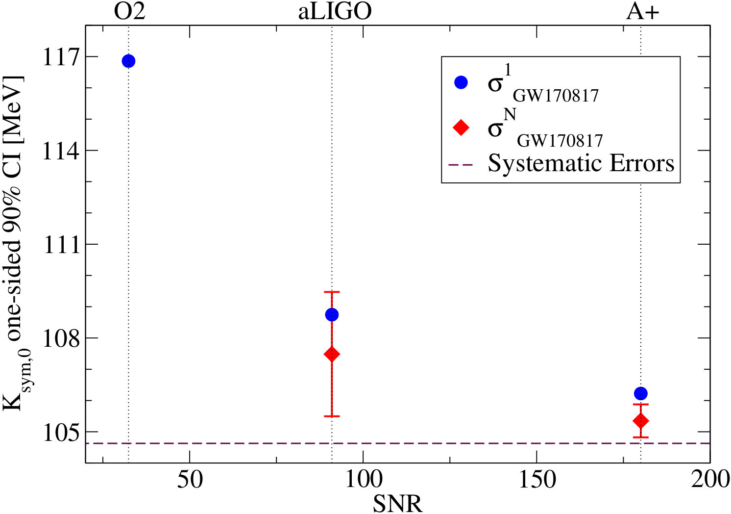 Figure 17
| Parameter | Fitting Function |
| [MeV] | |
| [MeV] | |
| [MeV] | |
| [MeV] | |
| [MeV] |
Peer Reviews
No public reviews on file for this paper yet. If you reviewed it on a platform where reviews are public (OpenReview, ICLR, NeurIPS, ICML), you can paste yours below so the community can read it here.
Videos
No videos yet. Explain this paper in a talk, walkthrough, or lecture? Add one.
Future Prospects for Constraining Nuclear Matter Parameters with
Gravitational Waves
Zack Carson
Department of Physics, University of Virginia, Charlottesville, Virginia 22904, USA
Andrew W. Steiner
Department of Physics and Astronomy, University of Tennessee, Knoxville, TN 37996, USA
Physics Division, Oak Ridge National Laboratory, Oak Ridge, TN 37831, USA
Kent Yagi
Department of Physics, University of Virginia, Charlottesville, Virginia 22904, USA
Abstract
The gravitational wave emission from the merging binary neutron star system GW170817 arrived full of tidal information which can be used to probe the fundamental ultra-dense nuclear physics residing in these stars. In previous work, we used two-dimensional correlations between nuclear matter parameters and tidal deformabilities of neutron stars applying specifically to GW170817 to derive constraints on the former. Here, we extend this analysis by finding similar correlations for varying chirp masses, the dominant determining factor in the frequency evolution of the inspiral, such that one can apply the same method to future detections. We estimate how accurately one can measure nuclear parameters with future gravitational wave interferometers and show how such measurements can be improved by combining multiple events. We find that bounds on the nuclear parameters with future observations can improve from the current one with GW170817 only by due to the existence of systematic errors caused mainly by the remaining uncertainty in the equation of state near and just above the nuclear saturation density. We show that such systematic errors can be reduced by considering multidimensional correlations among nuclear parameters and tidal deformabilities with various neutron star masses.
I Introduction
Neutron stars (NSs) exist in one of the most extreme states of matter found in the universe. However, the determination of the equation of state (EoS) of ultra-dense matter found exclusively in such compact objects remains to be one of the largest unsolved mysteries in both nuclear physics and astrophysics to date. The nuclear matter EoS determines many important stellar properties, such as the mass, radius, and tidal deformability, and is vital to the further study of supranuclear matter. Independent measurements of certain macroscopic NS observables determined by the EoS, such as the mass and radius, can be used to constrain the EoS, as was indeed done in Refs. Guver and Ozel (2013); Ozel et al. (2010); Steiner et al. (2010); Lattimer and Steiner (2014); Ozel and Freire (2016) via x-ray observations of the mass-radius relationship. However, such measurements potentially suffer from large systematic errors due to uncertainties in the astrophysical modeling of x-ray bursts.
Recent observations of gravitational waves (GWs) from a merging binary NS system (GW170817 Abbott et al. (2017a)) have been used to probe the interior nuclear structure via imprinted tidal effects Abbott et al. (2019, 2018a); Paschalidis et al. (2018); Burgio et al. (2018); Malik et al. (2018); Landry and Essick (2019), which offers us a cleaner method of determining the nuclear matter EoS than electromagnetic wave observations of neutron stars. As the NSs lose energy via GW emission, they inspiral towards each other and become increasingly tidally deformed in response to the companion stars’ tidal field. This deformation is characterized by the tidal deformability Flanagan and Hinderer (2008) of the NS, and is strongly dependent on the underlying EoS. Further, the mass-weighted combination of such tidal deformabilities from each star is the leading tidal parameter in the gravitational waveform, which has been constrained by the LIGO and VIRGO Collaboration to a 90% credible bound of Abbott et al. (2019); De et al. (2018). Such observations have also been mapped to the NS radius in Refs. Annala et al. (2018); Abbott et al. (2018a); Lim and Holt (2018); Bauswein et al. (2017); De et al. (2018); Most et al. (2018).
While all currently-proposed EoSs to date utilize various different approximations, one way to effectively study them is by measuring the nuclear parameters which parameterize the EoSs using a model-independent formalism. One such method for doing this111Piecewise polytropic constructions Read et al. (2009); Lackey and Wade (2015); Carney et al. (2018) and spectral EoSs Lindblom (2010); Lindblom and Indik (2012, 2014); Lindblom (2018); Abbott et al. (2018a) similarly parameterize nuclear matter EoSs in a model-independent way. See also Landry and Essick (2019); Kumar and Landry (2019) for related works on piecewise unified EoSs. is to Taylor expand the energy per nucleon of asymmetric nuclear matter about the saturation density of symmetric matter Myers and Swiatecki (1969); Vidaña et al. (2009). The resulting coefficients are known as the “nuclear matter parameters” and consist of the following: the slope of the symmetry energy ; the nuclear incompressibility ; the slope of the incompressibility ; the curvature of the symmetry energy ; and higher orders, each evaluated at the nuclear saturation density.
Previous important analyses by Alam et al. Alam et al. (2016) found approximately universal relations between the NS radius at a given mass and the nuclear parameters mentioned above (similar work can be found in Refs. Sotani et al. (2014); Silva et al. (2016)). Further, Malik et al. Malik et al. (2018) found that certain linear combinations of nuclear parameters (such as with chosen to give maximal correlation) gave way to heightened correlations with the individual tidal deformabilities evaluated at a given mass. By assuming individual masses for GW170817 and taking the approximate universal relations to be exact, the authors utilized prior constraints on the tidal deformability from GW170817 Abbott et al. (2017b); Radice et al. (2018) and Abbott et al. (2019); Oertel et al. (2017); Lattimer and Steiner (2014) to derive new constraints on the nuclear parameters.
In Ref. Carson et al. (2019a), we expanded upon the previous work of Malik et al. Malik et al. (2018) and found improved constraints on , , and . We made various improvements upon the original analysis, such as (i) using an expanded set of EoSs in order to fully take into account the EoS-variation systematic errors; (ii) considering the correlations with the mass-weighted tidal deformability (rather than , the tidal deformability at ) which was directly measured by GW observations; (iii) fully considering the EoS variation scatter uncertainty in the estimation of constraints; and (iv) adopting the full posterior distribution on as measured from GW170817. Further, we found that by using our method of computing the posterior distribution on nuclear parameters, high degrees of correlation between and such nuclear parameters was not necessary, as any covariances between the two was taken into account by the multi-variate Gaussian probability distribution between them. On the other hand, the authors of Ref. Malik et al. (2018) absolutely required high correlations with nuclear parameters in order to assume that the relationship between the tidal deformability and the nuclear parameters lie exactly on the best-fit line between the two. The resulting 90% confidence interval on the curvature of symmetry energy was found to be , which was more conservative than that derived in Ref. Malik et al. (2018).
Here, we extend the work of Ref. Carson et al. (2019a) into the future of GW astronomy. While every future merger event will be composed of NSs with varying individual masses which are difficult to measure, we can categorize them by the chirp mass , which is the dominant driving factor in the frequency evolution of the inspiral event given by a certain combination of individual NS masses. In this investigation, we repeat the analysis of Ref. Carson et al. (2019a) as a function of chirp mass, applicable to any future event. Further, we restrict the set of EoSs to those that obey the nuclear parameter correlations of Ref. Tews et al. (2017), and consider the implications of observations using future GW interferometers: Advanced LIGO (aLIGO) aLI , LIGO A+ (A+) Ap_ , Voyager Ap_ , Cosmic Explorer (CE) Ap_ , and Einstein Telescope (ET) ET . We will consider not only the increased sensitivities from current detectors but also the combined uncertainties from multiple-event detections (relevant for future detectors with expanded horizon volumes).
I.1 Executive summary
Here we summarize our results for busy readers. In the current analysis, we attempt to find constraints on the nuclear matter parameters as a function of the binary systems’ chirp mass. We begin by finding the correlations between the mass-weighted tidal deformability and various nuclear parameters, and combinations thereof. Similar to our results in Ref. Carson et al. (2019a), we find that the low-order nuclear parameters and observe small correlations with , while the correlations for higher-order parameter remains high at . For this reason, we consider constraints on the curvature of the symmetry energy which is one of the most uncertain parts of the EoS of dense nucleonic matter Li et al. (2019).
In this analysis, we compute the posterior probability distribution for the curvature of symmetry energy , for 22 different values of chirp mass between and . For each value of chirp mass considered, we compute the single-event uncertainties using Fisher analysis techniques. Approximated as a Gaussian prior, the uncertainty in may be used to estimate the posterior probability distribution on , by multiplication with the one-dimensional conditional probability distribution on given an observation of , and then integrating over all values. The process is then repeated for each value of chirp mass , resulting in a relationship between the uncertainties in and the chirp mass .
The corresponding one-sided 90% confidence intervals on for single-event detections, along with the calculated systematic errors, are plotted in Fig. 1 as a function of chirp mass for 6 different GW interferometers. In this figure, we observe that as the detector sensitivity is increased, the statistical errors become subdominant rather quickly. This in turn forces the overall errors to approach the systematic error “wall” at MeV, caused partially by uncertainties in the EoS at low-density which are less sensitive to neutron star tidal deformabilities. For this reason, the curves corresponding to the 3rd-generation detectors CE and ET become indistinguishable from the systematic errors – indicating the necessity to reduce such errors in order for the further constraint of to become possible.
Following this, we offer a method to further decrease the statistical errors in the measurement of . This is accomplished by repeating the same analysis for the fixed chirp mass of with the first coefficient, , of the Taylor expanded tidal deformability about 222 will remain fixed for the remainder of the analysis, with the exception of Sec. V, where we consider the effect of variations in ., rather than the mass-weighted tidal deformability . (or the tidal deformability at ) is mass-independent, and thus, it is identical for all future GW events. This way, we can combine the uncertainties for multiple detected events when it becomes applicable for future detectors. As was observed in Fig. 1, we found that the uncertainties in became dominated by systematics for the single-event analyses on Voyager-era detectors and beyond. By combining GW170817-like events detected on aLIGO and A+, we find that one can further reduce the statistical errors in such that the errors similarly become dominated by systematics.
Finally, we investigate the reduction of systematic errors by adding information about the tidal deformability at various different masses. We begin by generating a four-dimensional Gaussian probability distribution . The systematic error on is obtained by first evaluating at the fiducial values of , , and and estimating the 90% confidence interval. Figure 2 presents the systematic errors when is fixed to be , and () are varied between and . Observe how the resulting systematic uncertainties are reduced to MeV for certain combinations of and .
The remainder of this paper is organized as follows. We begin in Sec. II with a review on the tidal deformability of neutron stars, as well as the nuclear matter EoS and its constituent nuclear parameters. We follow this up in Sec. III with a study on the correlations between various nuclear parameters and the mass-weighted tidal deformability. In Sec. IV, we analyze the measurement accuracy on such nuclear parameters as a function of the chirp mass, applicable to future binary NS mergers. In Sec. V, we discuss how one can further reduce systematic errors by considering correlations among nuclear parameters and multiple tidal deformabilities at different NS masses. We conclude in Sec. VI with a discussion on the implications of our results, as well as an outline into possible avenues of future work. We have adopted geometric units such that throughout.
II Background and theory
In this section we begin with a review on the NS tidal deformability in Sec. II.1, followed up by a review on the NS equation of state and its constituent nuclear parameters in Secs. II.2 and II.3.
II.1 Neutron star tidal deformability
Here we offer a brief overview on how one can extract information on the internal structure of a NS by way of the GW observations of binary NS merger events, such as GW170817. In the presence of a neighboring tidal field (such as a NS in a binary system with a compact companion), NSs will acquire a quadrupole moment characterized as the linear response to :
[TABLE]
with tidal deformability Flanagan and Hinderer (2008); Hinderer (2008); Damour and Nagar (2009); Binnington and Poisson (2009); Yagi and Yunes (2013). The tidal deformability characterizes the NSs corresponding deformation from sphericity, and can be made unitless by the following normalization:
[TABLE]
with stellar mass .
Following Refs. Hinderer (2008); Damour and Nagar (2009); Yagi and Yunes (2013); Carson et al. (2019a), the dimensionless tidal deformability can be computed by isolating different asymptotic limits of the gravitational potential in the buffer zone given by
[TABLE]
where , is the length scale of the companion-induced curvature, and is the stellar radius. Here, corresponds to the -component of the full spacetime metric:
[TABLE]
constructed via a non-spinning, spherically-symmetric background solution perturbed by the tidal deformation with metric components . The perturbed Einstein equations may then be solved in the interior of the NS and matched to the exterior solution at the surface of the star. Further, the radius may then be determined from the condition .
In this investigation, we consider the scenario of two NSs orbiting each other in a binary system, like GW170817. In this case, each NS individually obtains quadrupole moments from the neighboring tidal field, resulting in two highly-correlated tidal deformabilities and . Due to these correlations, individual tidal deformabilities are very difficult to extract from GW observations. Typically, it is useful to reparameterize the waveform via independent linear combinations of and which enter the gravitational waveform at 5th post-Newtonian (PN) and 6PN orders333PN order corrections enter the gravitational waveform at relative powers of . respectively. The dominant tidal effect in the resulting waveform is known as the mass-weighted tidal deformability, and is given by Flanagan and Hinderer (2008)
[TABLE]
with mass ratio (). Here we also define the chirp mass of the binary system, which is the primary controlling factor of the merger inspiral defined by
[TABLE]
Similarly to , this quantity can be measured with much higher accuracy than either of the individual masses , , or the mass ratio . For this reason, we consider the binary chirp mass to be the dominant dependent variable in this analysis, cataloging our various results as a function of for any future GW event.
II.2 The nuclear matter parameters
While the NS EoS is not currently known, there are many methods one can use to restrict it using various observations. This is because the structure of a NS and many of its observables such as mass, radius, tidal deformability, etc. rely strongly on the underlying EoS of nuclear matter. For example, GW observations may help constrain the EoS in the pressure-density plane Abbott et al. (2018b). In this paper, we show how GW detections can aid in the constraint of various characteristics of the EoS, known as the nuclear matter parameters Vidaña et al. (2009).
As originally considered in Ref. Myers and Swiatecki (1969) and followed up in Refs. Vidaña et al. (2009); Alam et al. (2016); Malik et al. (2018); Carson et al. (2019a), we offer a generic method to parameterize NS EoSs. This is done by first Taylor expanding the energy per nucleon of asymmetric nuclear matter about (symmetric nuclear matter), where is the isospin symmetry parameter for nuclear matter with neutron density, proton density, and total density :
[TABLE]
Here and are the symmetric and second-order asymmetric nuclear matter energy per nucleon, respectively. Such energies are then further Taylor expanded about the nuclear saturation density as
[TABLE]
with . The above coefficients, all evaluated at the nuclear saturation density, determine the NS EoS and are referred to in the literature Myers and Swiatecki (1969); Vidaña et al. (2009) as the energy per particle ; incompressibility coefficient ; third derivative of symmetric matter ; the slope of the incompressibility Alam et al. (2016); Malik et al. (2018); symmetry energy ; its slope ; and its curvature .
In this paper, we expand upon previous works Alam et al. (2016); Malik et al. (2018); Carson et al. (2019a) and investigate the correlations between the mass-weighted tidal deformability and various nuclear parameters , , , and in order to derive constraints on such parameters. Specifically, we focus on the curvature of the symmetry energy , shown to be one of the most uncertain features of the nuclear matter EoS, especially at supranuclear densities found primarily in NSs Li et al. (2019).
II.3 The supranuclear equation of state
We now explain which EoSs we use in this paper. In Ref. Carson et al. (2019a), we showed the importance of considering a wide range of physically valid EoSs when computing constraints on nuclear parameters, in order to more properly take into account the systematic errors. In the current analysis, we employ a restricted set of the same EoSs as was used previously, taking into account the observed correlations between nuclear parameters and . Starting with the 121 nuclear EoS models found in Ref. Carson et al. (2019a), we further remove 63 EoS models which do not comply with the allowed regions shown in Fig. 8 of Tews et al. Tews et al. (2017). Here, they combined an exclusion region with the “accepted” 95.4% correlation confidence bands between and . See App. A for the impact of restricted EoSs on correlations between and .
Taking the shared region between the above two exclusions results in 58 different nuclear EoS models, which can be classified into 3 distinct classes: 13 non-relativistic “Skyrme-type” EoSs, 5 relativistic-mean-field (RMF) EoSs, and 40 EoS models developed with a phenomenological variation method (PEs). The Skyrme-type models used consist of: SKa, Sly230a Chabanat et al. (1997), Sly2, Sly9 Chabanat (1995), Sly4 Chabanat et al. (1998), SkOp Reinhard (1999), SK255, SK272 Agrawal et al. (2003), BSK20, BSK21 Goriely et al. (2010), BSK22, BSK24, BSK26 Goriely et al. (2013). Further, the RMF models used are: BSR2, BSR6 Dhiman et al. (2007); Agrawal (2010), NL3 Carriere et al. (2003), DD2 Typel et al. (2010), DDH Gaitanos et al. (2004). All 18 of the above EoSs originate from the minimal set of EoSs used in Refs. Alam et al. (2016); Malik et al. (2018), now restricted by nuclear matter correlations. Lastly, following Ref. Read et al. (2009), the high-density core-region of the EoSs used in our analysis are matched to the low-density crust-region of the SLy EoS model Douchin and Haensel (2001) at about half of the nuclear saturation density, .
One last class of EoSs indirectly used in our analysis can be found in Ref. Carson et al. (2019b), which we call “LVC constrained” EoSs in this paper. By sampling the full physical EoS parameter space, the LIGO and Virgo Collaboration Abbott et al. (2018b); Carney et al. (2018) derived a marginalized 90% posterior region on the NS pressure as a function of mass density (EoS) from GW170817, as seen in Fig. 2 of Abbott et al. (2018b). By randomly sampling the EoS posteriors from this analysis, a set of 100 “constrained” EoSs were obtained, restricted by the GW observation of GW170817. While we do not directly utilize these 100 EoSs in the current analysis, we use them to estimate the mean value of the mass-weighted tidal deformability in Sec. IV.1, seen by Fig. 6.
III Correlations between and nuclear parameters
We begin the current analysis by studying the correlations between the mass-weighted tidal deformability and various nuclear parameters , , and as was done in Ref. Carson et al. (2019a). In the previous analysis, we studied the correlations and constraints as a function of the mass ratio for the fixed chirp mass of ; corresponding to GW170817. We here supplement this investigation by considering the correlations and constraints as a function of varying chirp mass at a fixed mass ratio, applicable to any number of future GW observations. The left panel of Fig. 3 justifies the use of a fixed mass ratio by presenting as a function of for the various EoS models used in this analysis. Observe how is insensitive to the choice of . Such feature is absent in the right panel of Fig. 3, where is plotted as a function of chirp mass for fixed . Thus, for the remainder of this analysis we fix the mass ratio to be , corresponding to the center of derived in Ref. Coughlin et al. (2019) for GW170817.
We measure the amount of correlation between two observables and via
[TABLE]
with covariances given by
[TABLE]
Here represents the number of data points. A correlation of represents perfect correlation between observables and , while corresponds to no correlation.
In Ref. Carson et al. (2019a), we studied the universal relations between and various nuclear parameters , , in order to derive constraints on such parameters. Additionally, it was shown in Refs. Alam et al. (2016); Malik et al. (2018); Carson et al. (2019a) that certain linear combinations of nuclear parameters, specifically , , and , exhibit heightened correlations, allowing one to derive more accurate constraints on the individual nuclear parameters. However, it was found in Ref. Carson et al. (2019a) that this came at the expense of additional sources of uncertainty which, if properly accounted for, enlarges the resulting constraints on the nuclear parameters , , and . It was also found that the single nuclear parameters as well as the linear combinations involving and observed poor correlations of ; indicating somewhat unreliable constraints on the nuclear parameters.
Figure 4 similarly shows the above correlations as a function of chirp mass for a fixed mass ratio of . Observe how, similar to what was found in Ref. Carson et al. (2019a), the correlations for , , , and are exceedingly poor for all values of chirp mass. on the other hand, remains highly correlated with across the entire range of . We also observe how correlations are not improved by much when considering linear combinations between and .
Could other combinations of nuclear parameters give stronger correlations? To address this question, we further explore new combinations of nuclear parameters in App. B. In particular, we consider the “multiplicative” combinations of , , and that is motivated from Refs. Sotani et al. (2014); Silva et al. (2016). We found that such new combinations do not offer any advantages in terms of correlations and constraints.
For the above reasons, we consider only the curvature of the symmetry energy for the remainder of the investigation, without combinations with other parameters which would otherwise introduce additional uncertainties in the computation of constraints.
IV Nuclear parameter constraints with future GW observations
Now that we have identified the high-correlation behavior of , we proceed to compute projected bounds on the curvature of the symmetry energy as a function of chirp mass that is applicable to any future event. Additionally we offer the same analysis repeated for 5 anticipated future detector sensitivities for detectors O2 aLI , aLIGO aLI , A+ Ap_ , Voyager Ap_ , ET ET and CE Ap_ (see Fig. 5), which would allow one to compute the corresponding posterior distribution on given an events’ chirp mass .
IV.1 Single events
Previously in Ref. Carson et al. (2019a), a posterior distribution on as derived from GW170817, was utilized in order to compute posterior distributions on the nuclear parameters. In this analysis of future observations however, no such distribution is available. To remedy this, we approximate the effective “future” posterior distribution on as a Gaussian probability distribution given by
[TABLE]
for detector . Here, is computed from the mean value of the “LVC constrained” EoSs Carson et al. (2019b) described in Sec. II.3 for each value of chirp mass, as shown by Fig. 6. Further, is approximated via simple Fisher analyses (described below), which estimates the measurement accuracy on under the assumption of detector sensitivity . Figure 7 presents for all 6 detectors.
The Fisher analysis method Cutler and Flanagan (1994); Berti et al. (2005); Poisson and Will (1995) estimates the accuracy with which one can extract best-fit parameters given prior probability distributions and a template waveform . For this analysis, we consider the sky-averaged “IMRPhenomD” gravitational waveform template Khan et al. (2016); Husa et al. (2016) for point particles, modified by the 5PN and 6PN tidal corrections given in Ref. Wade et al. (2014). We utilize a template parameter vector consisting of
[TABLE]
where is a normalized amplitude factor, is the luminosity distance to the event, is the redshifted chirp mass, is the symmetric mass ratio, are the symmetric and anti-symmetric combinations of individual spins , and is a tidal parameter entering first at 6PN order. In this investigation, we utilize fiducial parameter values of , , , , and are chosen from the current chirp mass iteration with a mass ratio of , and is computed from the mean value of the “LVC constrained” EoSs. Additionally, we impose Gaussian spin priors of , and tidal priors of , and Wade et al. (2014).
To obtain a posterior distribution, one needs to know both the likelihood and prior distributions. Assuming the prior distributions on template parameters are Gaussian444A more comprehensive Bayesian analysis assumes the more valid choice of uniform prior distributions., the resulting posterior distributions are also Gaussian with root-mean-squares of
[TABLE]
The Fisher matrix is defined as
[TABLE]
where are the prior root-mean-square estimates of parameters , and the inner product is given by
[TABLE]
Now that all of the tools are prepared, we next compute the posterior distributions on using the Gaussian prior distributions on computed above as a function of chirp mass, for future detectors. Following the process used in Ref. Carson et al. (2019a), this is accomplished by first generating a two-dimensional Gaussian probability distribution between and , taking into account the covariances between the two as
[TABLE]
Here and are the 2D vectors containing and their means respectively, and is the covariance matrix with elements given by Eq. (10).
Let us now offer readers the means to fully reproduce the results of the above analysis for any future event by constructing a fit for and in terms of chirp mass . Based on the relations between the former and the latter as shown in Fig. 8, we create a fit in a logarithmic power expansion as
[TABLE]
with being the various parameters and , and fitting coefficients , , and which are summarized in Table 1. Observe how well the fit agrees with the numerical data in Fig. 8.
Constraints on are extracted by first computing the conditional probability distributions on given a tidal deformability observation of . By following Ref. Jensen (2007), we can generate the one-dimensional conditional probability distribution on by taking
[TABLE]
Above, is the normal distribution with mean and variance and , while and are the mean and variances of and . Finally, we can combine the one-dimensional conditional probability distribution function of Eq. (18) with the one-dimensional prior distribution on of Eq. (11). Marginalizing over results in a posterior probability distribution on
[TABLE]
from which 90% confidence intervals on the curvature of symmetry energy can be extracted. This process is then repeated for values of chirp mass across its feasible range, and then for each interferometer . Appendix C exemplifies this by demonstrating the procedure for one value of chirp mass on interferometer O2, corresponding to GW170817. The results found there are compared to those found in Ref. Carson et al. (2019a) in order to demonstrate the accuracy of our approximated Gaussian priors, rather than the full posterior distribution found in Ref. Abbott et al. (2018b). We found that we slightly underestimate the errors in by using this method.
There is one important question to analyze here: how do the statistical errors on ( in given in Eq. (11) that enters in Eq. (19)) compare to the systematic errors (covariance in given in Eq. (16) that also enters in Eq. (19))? As more events are observed and the detector sensitivities drop, the statistical errors on the measurement of approach zero, and the overall errors limit closer to the systematic error “wall” introduced from the EoS variation in the universal relations. We study this effect by first plotting the overall errors on as a function of chirp mass, defined to be the one-sided 90% confidence interval on the posterior distribution of . Following this, we define the systematic errors to be the one-sided 90% confidence interval of in the two-dimensional probability distribution evaluated at the central value of the prior distribution shown in Fig. 6. Equivalently, the fixed diagonal coefficient of the Gaussian argument shows the systematic errors to be exactly equal to .
Figure 1 displays the results of the above described procedure; plotting the (one-sided 90% confidence interval) overall and systematic errors on the measurement of as a function of chirp mass. We observe here the presence of a minimum in the uncertainties with respect to the chirp mass - a relic originating from the correlations between and seen in Fig. 4, which similarly observe a maximum at the same chirp mass (and thus minimum EoS variation that generates systematic errors). We do note, however, that while previous analyses by Refs. Alam et al. (2016); Malik et al. (2018) required high correlations for the computation of constraints555Refs. Alam et al. (2016); Malik et al. (2018) assumed the relationship between (the tidal deformability at ) and nuclear parameters to lay exactly on the best-fit line between the two. Thus, high degrees of correlation were absolutely necessary for accuracy on this claim., our analysis does not, as all covariances between and are taken into account by the two-dimensional probability distribution of Eq. (16).
Observe also how, as predicted, the statistical errors drop as the more sensitive detectors are analyzed, reducing to almost zero as the overall errors limit to the fixed systematic error “wall”. The overall errors on the highly-sensitive third generation interferometers CE and ET are indistinguishable from the systematic errors – indicating that the error budget is highly dominated by systematics at this point. Once the errors are dominated by systematics, improving detector sensitivities or observing new events will not aid in the further constraint of . This indicates the urgent need to reduce the systematic errors found in the EoS-variation of the universal relations for the Voyager-class detectors and beyond666A similar conclusion was reached in Ref. Carson et al. (2019b), where the detector statistical errors became comparable to the systematic errors from the binary Love universal relations for future detectors Voyager and beyond..
IV.2 Multiple events
The future of GW astronomy will become quite busy in terms of detected events. For example, future GW interferometer Cosmic Explorer will be detecting anywhere from to Carson et al. (2019b) binary NS merger events within its horizon distance per year - a staggering number which will certainly help reduce the statistical errors on tidal measurements. How does one account for this effect when studying the uncertainties in future, undetected, events? The dominant tidal parameter in the gravitational waveform, , depends strongly on the subsequent masses in the binary system, something difficult to predict beforehand. Ultimately, this prevents one from combining the uncertainties on for multiple events.
Fortunately, this can be remedied by following in the footsteps of Ref. Carson et al. (2019b), where we reparameterized the gravitational waveform to instead consider the and tidal coefficients, generated by Taylor expanding the tidal deformability about the reference mass of Del Pozzo et al. (2013); Yagi and Yunes (2016):777We note here that a linear truncation of this Taylor series is valid for our purposes. By taking into account an additional quadratic term identified by , we found a reduction in measurement accuracy in by only , across various detectors and values of chirp mass.
[TABLE]
Here, and are the dimensionless tidal deformability and its slope at , and they do not depend on the individual NS masses or any combination thereof (however they do depend on the fiducial mass value chosen). Therefore, they are identical for every future binary NS merger event, and may be combined in uncertainty.
Similar to the correlation between and , we also find a correlation between and . We constructed a 2D Gaussian distribution similar to in Eq. (16) and find
[TABLE]
for . Notice that both and are independent of in this case.
In this section, we repeat the analysis performed in Sec. IV.1 using the combined uncertainties on from unique events with chirp mass , corresponding to the number of observed binary NS mergers within one observing year on detector . We refer to App. D for details on how to combine information from multiple events, which closely follows App. A of Carson et al. (2019b). Fiducial values of and were computed to be the mean values of and from the “LVC constrained” EoSs. Figure 9 shows how the combined-event uncertainties on for the fixed chirp mass of further become saturated on the aLIGO, and A+ detectors as well. As was shown in Fig. 1, the single-event uncertainties on become dominated by systematic errors for Voyager-class detectors and beyond, and thus there is not much point in stacking multiple events for these detectors to further reduce statistical errors on .
V Reducing systematic errors via multidimensional correlations
Let us now consider how we can reduce the systematic “walls” present in Fig. 1. In Sec. IV.2, this was computed by evaluating the two-dimensional probability distribution between and at the fiducial value of , and then finding the 90% confidence interval of the resulting probability distribution of to yield MeV. We here construct multidimensional correlations among and at a few different masses (since we expect to detect GWs from binary NSs with different masses with future observations) to see how adding information of the tidal deformability at multiple different masses may help us to reduce the systematic errors on .
Let us begin by using at two different masses and . This requires us to find a three-dimensional correlation among , , and , and construct a three-dimensional Gaussian distribution . Figure 10 shows an example of such a distribution for the case of and . The systematic error is then computed by evaluating the three-dimensional distribution at the fiducial values of and , and then evaluating the resulting one-dimensional probability distribution at the 90% confidence interval.
Figure 11 displays the resulting systematic uncertainties on using canonical masses and between and . Observe that the systematic errors can be reduced by setting both and to be large or small. However, this means that , which corresponds to effectively using a two dimensional probability distribution. Thus, in this case, having additional information on at a different mass does not help to reduce the systematic errors.
It may sound strange that adding more pieces of information does not help to reduce the systematic errors. Let us explain why this is the case by comparing the systematic errors at and . Figure 12 compares the two-dimensional 90% contours between and from two different methods by computing (i) directly the two-dimensional probability distribution from Eq. (16), and (ii) the three-dimensional probability distribution between , , and , and then evaluating it at the fiducial value of . We observe that while the contour from the first case has a larger area (and value of ) as expected due to the use of less information, it becomes distorted such that the systematic uncertainty (along the dashed horizontal line corresponding to the fiducial value of ) becomes smaller than that from the first case.
Let us now consider using at three different masses, , and . This requires us to find a four-dimensional correlation and construct the four-dimensional Gaussian probability distribution . We fix , and allow and to vary between . Similar to the process used previously, this probability distribution is evaluated at the fiducial values of , and :
[TABLE]
The resulting 90% confidence intervals are presented in Fig. 2 for the entire range of and mass values. We observe that by including information about binaries with large, medium, and small masses together, the systematic errors can be improved drastically, down to MeV. We also see that along the diagonal line of , the four-dimensional probability distribution reduces to the three-dimensional case , with uncertainties MeV approaching that of Fig. 11 along the horizontal dashed line.
VI Discussions
Are there any other ways to further improve the constraints on using observed GW events? One might think that the constraint on with GW170817 may help in this direction. However, the restriction of data in only the dimension does not help as systematic errors are found by evaluating the scattering width in the direction.
Finally, we briefly discuss the possibility of NSs with strong first-order phase transitions from hadronic to quark matter in the core, as described in Ref. Paschalidis et al. (2018). With high enough observed chirp masses , future binary NS merger events could potentially be composed of one or both hybrid stars (HSs) with quark-matter cores. The tidal deformabilities and thus, the nuclear parameters, depend on such structure, and could potentially disagree between events with varying chirp masses and combinations of NS/HS Montana et al. (2019). Thus, significant variations between nuclear parameter measurements with future GW observations with varying chirp masses could potentially present evidence of strong phase transitions at around times the nuclear saturation density. If such transitions are present at sufficiently low-densities, then the nuclear matter parameters will be further decoupled from the GW observations and thus our lower limit for the nuclear matter parameter uncertainties will increase. Alternatively, similar measurements of nuclear parameters could either indicate a pure hadronic matter EoS, or phase transitions occurring at higher nuclear densities. The structure of such high-density transitions could be probed by the GW post-merger oscillation signal.
As we showed in the previous section, one can use multidimensional correlations to reduce the systematic errors. Instead of using tidal deformabilities from different NS masses obtained from GWs alone, one can consider combining information from multi-messenger observations. For example, pulse profiling techniques by NASA’s Neutron star Interior Composition Explorer (NICER) instrument may provide high-precision measurements on the NS radius down to Ozel et al. (2016); Sieniawska et al. (2018). Thus, one can construct multidimensional correlations among nuclear parameters, tidal deformabilities and radii of NSs. The work along this direction is currently in progress Schumacher et al. (tion).
Acknowledgments
We thank David Nichols for his illuminating advice on conditional probability distributions. Z.C. and K.Y. acknowledge support from NSF Award PHY-1806776. K.Y. would like to also acknowledge networking support by the COST Action GWverse CA16104. A.W.S. was supported by NSF grant PHY 1554876 and by the U.S. DOE Office of Nuclear Physics.
Appendix A Original versus restricted sets of EoS
In this appendix, we show how the restriction of EoSs described in Sec. II.3 used in the current analysis impacts our observations, as compared to the original set of EoSs used in Ref. Carson et al. (2019a). Figure 13 shows a comparison between the two-dimensional probability distributions resulting from each set of EoSs. We see that while the restriction to EoSs does indeed shrink the 90% confidence intervals in the direction of correlation, the widths are approximately equal at the fiducial value of (where the systematic errors are analyzed). This shows that while using a subset of EoSs may reduce the overall error888We indeed observed large reductions in the overall errors found in Fig. 1 when using the restricted EoSs rather than the original ones, while the level of systematics stayed constant at MeV., the level of systematic errors will remain mostly fixed. Our result is consistent, for example, with Ref. Carriere et al. (2003), which found that the correlation between and the radius of a neutron star was weak because of the contribution of the high-density component of the EoS.
Appendix B Multiplicative combinations of nuclear parameters
In this appendix, we discuss the feasibility of using multiplicative combinations of nuclear parameters, such as , rather than the linear combinations such as considered in Refs. Alam et al. (2016); Malik et al. (2018); Carson et al. (2019a). Here we consider the following multiplicative combinations for comparison purposes: , , and , where coefficients , , and are similarly chosen to achieve maximal correlation. Such multiplicative combinations are similar to those considered in Sotani et al. (2014); Silva et al. (2016).
Figure 14 presents the correlations between and all 6 multiplicative and linear combinations of nuclear parameters considered in this analysis. While the two classes of nuclear parameter combinations produce very similar correlations with , we observe that the linear cases slightly outperform the multiplicative cases for nearly all values of chirp mass. Similarly, repeating the analysis999Because the two-dimensional probability distribution is now between and , an additional marginalization over : must be performed ( is an additional prior distribution on given by Refs. Lattimer and Lim (2013); Lattimer and Steiner (2014); Tews et al. (2017); Oertel et al. (2017)) in order to extract the posterior distribution on . found in Sec. IV returns constraints on to be slightly worse than that considered in the the main analysis, due to the additional inclusion of uncertainties from nuclear parameter . One arrives at a similar conclusion if one uses a linear combination with Carson et al. (2019a).
From this evidence, we conclude with the remarks that the multiplicative combinations of nuclear parameters offer nothing new in terms of enhanced constraints on nuclear parameters. The multiplicative combinations of nuclear parameters slightly under-perform their linear combination counterparts in terms of correlations with . Thus, we neglect their use and continue our analysis as was done previously in Carson et al. (2019a).
Appendix C Example computation of the posterior distribution
In this appendix, we demonstrate the process of computing the posterior distribution on (used in Sec. IV) for one value of chirp mass, , corresponding to GW170817 on detector O2. This case corresponds to the large dot in Fig. 1. Referring to Figs. 6 and 7, we observe that the mean and root-mean-square values for O2 detector sensitivity at are given by and , respectively. This results in a prior distribution on shown in Fig. 15, given by
[TABLE]
We additionally show the true posterior distribution on derived in Ref. Abbott et al. (2018b), which was used as a prior in our original analysis found in Ref. Carson et al. (2019a) for comparison purposes.
Following along with Sec. IV.1, we generate the two-dimensional probability distribution between and , given by Eq. (16). We find the covariance matrix and the mean vector to be
[TABLE]
for This results in the two-dimensional probability distribution between and shown in Fig. 16. The systematic error on is then computed by evaluating the 90% confidence interval width of the distribution in the -dimension at , corresponding to the mean of the prior distribution in . The resulting (one-sided 90% confidence level) systematic errors for this case are found to be .
Next, we obtain the one-dimensional conditional probability distributions on given tidal deformability observations of . By following Eq. (18), this is simply given by
[TABLE]
Finally, the posterior distribution on can be computed by combining the one-dimensional conditional probability distributions with the prior distribution on , and then integrating over all observations of :
[TABLE]
Figure 17 finally displays the resulting posterior distribution on , with a mean value of , giving a 90% confidence interval of (or a one-sided confidence interval of MeV corresponding to the maroon dot in Fig. 1). Comparing this to the resulting posterior distribution (also shown in Fig. 17) found in Ref. Carson et al. (2019a) giving a 90% confidence interval of , we find that this approximation of priors slightly underestimates the errors in , but otherwise works quite well. We also see that this approximation of priors skews the distribution less so than the LVC posterior, making it more normally distributed. We also note that here, we utilize a restricted set of EoSs compared to that done in Ref. Carson et al. (2019a), resulting in a slightly more accurate posterior distribution on .
Appendix D Combining uncertainties from multiple events
In this appendix, we explain how one can combine statistical uncertainties on certain parameters from multiple events. We closely follow App. A of Carson et al. (2019b). To estimate the number of detected binary NS merger events on interferometer , we integrate the local binary NS merger rate across all redshift values within detector ’s horizon redshift with SNR thresholds of . Following the process used in Ref. Carson et al. (2019b), this is given by
[TABLE]
In our cosmology, we choose , , and to be
[TABLE]
[TABLE]
[TABLE]
where is the local Hubble constant, is the universe’s vacuum energy density, is the local binary NS coalescence rate density Abbott et al. (2017b), and is chosen to be a one year observation period. Doing so gives the rates found in Table VIII of Ref. Carson et al. (2019b). For demonstration purposes, we choose to use the lower and upper limits of these rates which are found to be , , , , and events per year for aLIGO, A+, Voyager, CE, and ET respectively.
Similarly following Ref. Carson et al. (2019b), the combined uncertainty is computed by first simulating a population of events from the SNR () probability distribution: Schutz (2011); Chen and Holz (2014)
[TABLE]
with an SNR threshold of . The combined population root-mean-square error on is then computed by integrating over all sources at various redshifts :
[TABLE]
Here, is the redshift dependence of the root-mean-square error on detector , evaluated via Fisher analyses at various redshifts up to .
The reference list from the paper itself. Each links out to its DOI / PubMed record.
- 1Guver and Ozel (2013) T. Guver and F. Ozel, Astrophys. J. 765 , L 1 (2013) , ar Xiv:1301.0831 [astro-ph.HE] . · doi ↗
- 2Ozel et al. (2010) F. Ozel, G. Baym, and T. Guver, Phys.Rev. D 82 , 101301 (2010) , ar Xiv:1002.3153 [astro-ph.HE] . · doi ↗
- 3Steiner et al. (2010) A. W. Steiner, J. M. Lattimer, and E. F. Brown, Astrophys.J. 722 , 33 (2010) . · doi ↗
- 4Lattimer and Steiner (2014) J. M. Lattimer and A. W. Steiner, The European Physical Journal A 50 (2014), 10.1140/epja/i 2014-14040-y . · doi ↗
- 5Ozel and Freire (2016) F. Ozel and P. Freire, Ann. Rev. Astron. Astrophys. 54 , 401 (2016) , ar Xiv:1603.02698 [astro-ph.HE] . · doi ↗
- 6Abbott et al. (2017 a) B. P. Abbott et al. (Virgo, LIGO Scientific), Phys. Rev. Lett. 119 , 161101 (2017 a) , ar Xiv:1710.05832 [gr-qc] . · doi ↗
- 7Abbott et al. (2019) B. P. Abbott et al. (LIGO Scientific, Virgo), Phys. Rev. X 9 , 011001 (2019) , ar Xiv:1805.11579 [gr-qc] . · doi ↗
- 8Abbott et al. (2018 a) B. P. Abbott et al. (LIGO Scientific, Virgo), Phys. Rev. Lett. 121 , 161101 (2018 a) , ar Xiv:1805.11581 [gr-qc] . · doi ↗