Iteration-complexity and asymptotic analysis of steepest descent method for multiobjective optimization on Riemannian manifolds
Orizon P. Ferreira, Maur\'icio S. Louzeiro, Leandro F. Prudente

TL;DR
This paper analyzes the convergence and complexity of the steepest descent method for multiobjective optimization on Riemannian manifolds, providing theoretical bounds and numerical validation for various stepsize strategies.
Contribution
It introduces iteration-complexity bounds and asymptotic analysis for the steepest descent method on Riemannian manifolds with multiple stepsize rules, a novel extension in this context.
Findings
The method converges under different stepsize strategies.
Complexity bounds are established for each stepsize rule.
Numerical experiments confirm theoretical results.
Abstract
The steepest descent method for multiobjective optimization on Riemannian manifolds with lower bounded sectional curvature is analyzed in this paper. The aim of the paper is twofold. Firstly, an asymptotic analysis of the method is presented with three different finite procedures for determining the stepsize, namely, Lipschitz stepsize, adaptive stepsize and Armijo-type stepsize. The second aim is to present, by assuming that the Jacobian of the objective function is componentwise Lipschitz continuous, iteration-complexity bounds for the method with these three stepsizes strategies. In addition, some examples are presented to emphasize the importance of working in this new context. Numerical experiments are provided to illustrate the effectiveness of the method in this new setting and certify the obtained theoretical results.
Click any figure to enlarge with its caption.
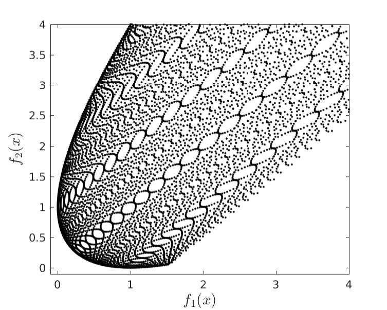 Figure 1
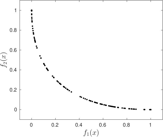 Figure 2
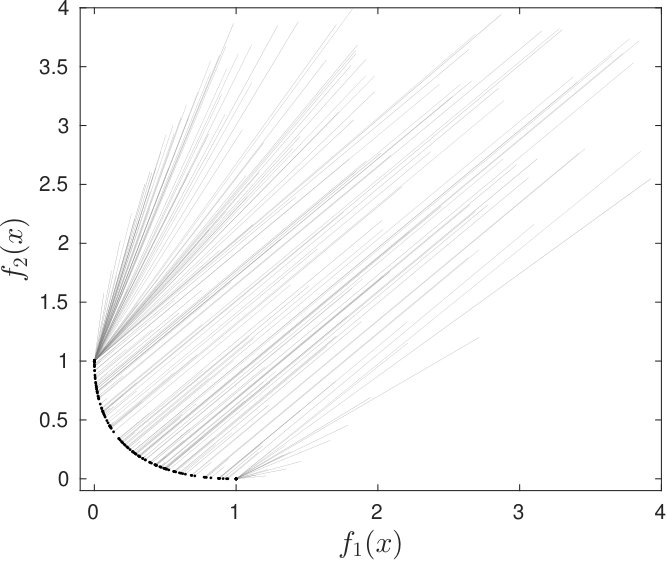 Figure 3
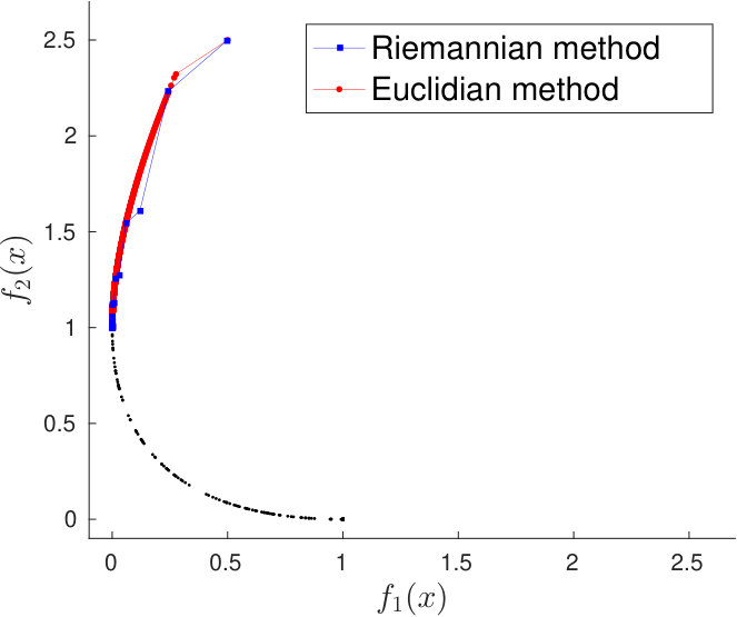 Figure 4
| it | evalf | evalg | ||
|---|---|---|---|---|
| Riemannian method | 100.0 | 5.0 | 49.0 | 12.0 |
| Euclidean method | 95.1 | 1629.0 | 5721.0 | 3260.0 |
| it | evalf | evalg | |||
|---|---|---|---|---|---|
| 10 | 2 | 100.0 | 26.5 | 117.5 | 55.0 |
| 100 | 2 | 100.0 | 71.5 | 220.0 | 145.0 |
| 400 | 2 | 100.0 | 273.0 | 622.0 | 548.0 |
| 1000 | 2 | 100.0 | 17.0 | 104.0 | 36.0 |
| it | evalf | evalg | |||
|---|---|---|---|---|---|
| 5 | 2 | 100.0 | 8.0 | 26.5 | 18.0 |
| 10 | 2 | 100.0 | 13.0 | 38.5 | 28.0 |
| 20 | 2 | 100.0 | 18.0 | 49.0 | 38.0 |
| 50 | 2 | 100.0 | 27.0 | 64.0 | 56.0 |
Peer Reviews
No public reviews on file for this paper yet. If you reviewed it on a platform where reviews are public (OpenReview, ICLR, NeurIPS, ICML), you can paste yours below so the community can read it here.
Videos
No videos yet. Explain this paper in a talk, walkthrough, or lecture? Add one.
Iteration-complexity and asymptotic analysis of steepest descent method for multiobjective optimization on Riemannian manifolds
O. P. Ferreira IME/UFG, Avenida Esperança, s/n, Campus Samambaia, Goiânia, GO, 74690-900, Brazil (e-mails: [email protected], [email protected]).
M. S. Louzeiro TU Chemnitz, Fakultät für Mathematik, D-09107, Chemnitz, Germany (e-mail: [email protected]).
L. F. Prudente 11footnotemark: 1
Abstract
The steepest descent method for multiobjective optimization on Riemannian manifolds with lower bounded sectional curvature is analyzed in this paper. The aim of the paper is twofold. Firstly, an asymptotic analysis of the method is presented with three different finite procedures for determining the stepsize, namely, Lipschitz stepsize, adaptive stepsize and Armijo-type stepsize. The second aim is to present, by assuming that the Jacobian of the objective function is componentwise Lipschitz continuous, iteration-complexity bounds for the method with these three stepsizes strategies. In addition, some examples are presented to emphasize the importance of working in this new context. Numerical experiments are provided to illustrate the effectiveness of the method in this new setting and certify the obtained theoretical results.
Keywords: Steepest descent method, multiobjective optimization problem , Riemannian manifold, lower bounded curvature, iteration-complexity bound.
**AMS ** subject classification: 90C33, 49K05, 47J25.
1 Introduction
A constrained multiobjective optimization problem with constraint set , consists of objective functions , that have to be optimized at the same time on . In recent years, there has been a significant increase in the number of papers addressing this class of problems; for example, see [1, 2, 3, 4, 5, 6, 7]. Here, among the methods designed for solving multiobjective optimization problems, we are interested in the steepest descent method. This method, was proposed in [8] and since of then several variants have been considered, including but not limited to [9, 10, 11, 12, 13, 14]. Recently some iteration-complexity results to gradient method for unconstrained multi-objective optimization problem were presented in [15]. These results have been shown to be the same global rates as for steepest descent method in scalar objective optimization.
Constrained optimization problems, where the constraint set can be endowed with Riemannian manifold structure, have been studied extensively in the last few years. Some aspects about the use of Riemannian geometry tools to study these class of problems arises from the following interesting fact. Endowing with a suitable Riemannian metric, an Euclidean non-convex constrained problem with constraint set can be seen as a Riemannian convex unconstrained problem. In addition to this property, for differentiable functions, its gradient can also become Riemannian Lipschitz continuous; see [16]. Consequently, the geometric and algebraic structures that come from the Riemannian metric make possible to greatly reduce the computational cost for solving such problems. Indeed, it is well known that the iteration-complexity of several optimization methods for convex optimization problems such that objective functions have Lipschitz continuous gradient is much lower than nonconvex optimization problems; see for example [17, 18, 19, 20, 21] and references therein. Furthermore, many optimization problems are naturally posed on the Riemannian context; see [22, 18, 23, 20]. Then, to take advantage of the intrinsic Riemannian geometric structure, it is preferable to treat these problems as the ones of finding singularities of gradient vector fields on Riemannian manifolds rather than using Lagrange multipliers or projection methods; see [24, 23, 25]. In this sense constrained optimization problems can be seen as unconstrained from the point of view of Riemannian geometry. Moreover, intrinsic Riemannian structures can also opens up new research directions that aid in developing competitive optimization algorithms; see [26, 22, 18, 27, 23, 20]. More about concepts and techniques of optimization on Riemannian context can be found in [28, 29, 30, 31, 32, 21, 33, 25, 34] and the bibliographies therein.
In this paper we will study the steepest descent method for multiobjective optimization on Riemannian manifolds. The aim is twofold. First, asymptotic analysis will be done for quasi-convex and convex vectorial functions. In fact, in [35] asymptotic analysis of this method has already been done in Riemannian context; see also [36]. However, the analysis asymptotic presented in these previous works is just to stepsize given by Armijo rule and it demand that the Riemannian manifolds have nonnegative sectional curvature. The asymptotic analysis presented in the present paper increase the previous ones in two different aspects. It is provided an analysis with three different finite procedures for determining the stepsize, namely, Lipschitz stepsize, adaptive stepsize and Armijo-type stepsize and only lower boundedness of the curvature of the Riemannian manifold is assumed. The second aim is to present iteration-complexity bounds for steepest descent method for multiobjective optimization on Riemannian manifolds. It is worth noting that, our results generalize to the Riemannian context the results obtained in [15]. Besides, we present one iteration-complexity bound that is new even in Euclidean setting. In addition, some examples are presented to emphasize the importance of working in this new context. Numerical experiments are provided to illustrate the effectiveness of the method in this new setting and certify the obtained theoretical results.
The organization of this paper is as follows. In Section 2, some notations and auxiliary results, used throughout of the paper, are placed. In Section 3, we present the algorithm and the stepsizes that will be used. In Section 3.1, the asymptotic convergence analysis of the sequence generated by the steepest descent method is made. In Section 3.2, we present iteration-complexity bounds related to the steepest descent method. In Section 4, we present examples of vectorial convex functions with componentwise Lipschitz continuous Jacobian. Numerical experiments are present in Section 5. Finally, some conclusions are given in Section 6.
2 Notations and Auxiliary Concepts
In this section, we recall some concepts, notations, and basics results about Riemannian manifolds and vector optimization. For more details we refer the reader to [37, 38, 25, 19].
We denote by the tangent space of a finite dimensional Riemannian manifold at , and by tangent bundle of . The corresponding norm associated to the Riemannian metric is denoted by . We use to denote the length of a piecewise smooth curve . The Riemannian distance between and in is denoted by . Denote by , the space of smooth vector fields on . Let be the Levi-Civita connection associated to . For each and a piecewise smooth curve , the covariant derivative induces an isometry, relative to , defined by , where is the unique vector field on the curve such that and , the so-called parallel transport along of joining to . When there is no confusion, denotes the parallel transport along the segment joining to . Given that the geodesic equation is a second order nonlinear ordinary differential equation, then the geodesic is determined by its position and velocity at . The restriction of a geodesic to a closed bounded interval is called a geodesic segment. For any two points , denotes the set of all geodesic segments with and . A geodesic segment joining to in is said to be minimal if its length is equal to . In this paper, all manifolds are assumed to be connected, finite dimensional, and complete. Hopf-Rinow’s theorem asserts that any pair of points in a complete Riemannian manifold can be joined by a (not necessarily unique) minimal geodesic segment. Owing to the completeness of the Riemannian manifold , the exponential map is given by , for each . For a differentiable function on , the Riemannian metric induces the mapping which associates its gradient via the following rule , for all and . For a twice-differentiable function, the mapping associates its hessian via the rule , for all , where the last equalities imply that , for all . Let us to introduce some concepts of vector optimization on a Riemannian manifold . Letting define and . For , (or ) means that and (or ) means that . Let be a differentiable function. We denote the Riemannian jacobian of at a point by , where , and the image of the Riemannian jacobian of at by A vectorial function is said to be convex on if for any and the composition satisfies for all By convexity of , it follows that . A vectorial function is called quasi-convex on if, for every and , it holds , for all , where the maximum is considered coordinate by coordinate. It is immediate of the above definitions that if is convex then it is quasi-convex. Moreover, if is a quasi-convex function, than implies .
The next result plays an important role in next sections. Its proof, which will be omitted here, follows the same ideas as those presented in the proof of [30, Lemma 3.2], with some minor technical adjustments needed to settle it to our goals. For simplifying our notations throughout the paper, we define
[TABLE]
Lemma 1**.**
Let be a complete Riemannian manifolds with sectional curvature . Let , , , be defined by and be a minimizing geodesic with and . Then, for any there holds
[TABLE]
and, consequently, the following inequality holds
[TABLE]
Next we present the definition of Lipschitz continuous gradient vector field; see [39].
Definition 2**.**
Let be a differentiable function on the set . The gradient vector field of is said to be Lipschitz continuous on with constant if, for any and , it holds that
The norm of the hessian at is given by
[TABLE]
The next result has similar proof to its Euclidean version and it will be omitted.
Lemma 3**.**
Let be a twice continuously differentiable function. The gradient vector field of is Lipschitz continuous with constant if, and only if, there exists such that , for all .
In the following we present the concept of Lipschitz continuity for the Riemannian Jacobian of a vectorial function.
Definition 4**.**
Let be a differentiable function. If for each there exists a such that , for any and , then we say that is componentwise Lipschitz continuous on with constant .
The proof of the next lemma follows, with appropriate adjustments, the same idea of proof of the scalar version presented in [17, Corollary 2.1]. Throughout of the paper we will use the following notation
[TABLE]
Lemma 5**.**
Let be a differentiable function. Assume that is componentwise Lipschitz continuous on with constant and . Then there holds
[TABLE]
Next we introduce the concept of quasi-Fejér convergence, which played an important role in the analysis of the gradient method.
Definition 6**.**
A sequence in the complete metric space is quasi-Fejér convergent to a set if, for every , there exist a sequence such that , , and , for all .
In the following we state the main property of the quasi-Fejér concept, its proof follows the same path as its Euclidean counterpart proved in [40], by replacing the Euclidean distance by the Riemannian one.
Theorem 7**.**
Let be a sequence in the complete metric space . If is quasi-Fejér convergent to a nonempty set , then is bounded. Furthermore, if a cluster point of belongs to , then .
Hereafter, we assume that is a complete Riemannian manifolds with sectional curvature , where . We point out that for Riemannian manifold with nonnegative sectional curvature, the convergence analysis of the steepest descent method for convex and quasi-convex vector functions is well understood; see for example [35, 36].
3 Steepest Descent for Multiobjective Optimization
Let be a continuously differentiable function. The problem of finding an optimum Pareto point of , we denote by
[TABLE]
A point satisfying is called critical Pareto. An optimum Pareto point of is a point such that there exists no other with and . Moreover, a point is a weak optimal Pareto of if there is no with . Consider the following problem
[TABLE]
Whenever is not critical Pareto, the optimization problem (3) has only one solution, which is called steepest descent direction for in and it is denoted by
[TABLE]
In the next lemma we state an important property of the steepest descent direction. Its proof can be found in [35, Lemma 5.1].
Lemma 8**.**
The steepest descent direction mapping , is a continuous vector field.
Moreover, the vector is the solution of the problem (3) if and only if there exist , for , such that
[TABLE]
see [35, Lemma 4.1]. In the following lemma we state an important inequality for our convergence analysis and an equivalence for a point to be a critical Pareto.
Lemma 9**.**
Let and as defined (4). Then,
[TABLE]
Consequently, In addition, is critical Pareto point of if, and only if, .
Proof.
Let and as in (4). Thus, from the first equality in (5) we have
[TABLE]
Hence, by the definition of and the second equality in (5), it is easy to verify that (6) holds. The second statement follows by using the definitions of and . We proceed with the prove of the third statement of the lemma. Assuming that is a critical Pareto, it follows from the definition that there exists such that . Then, the by first part of lemma we have . The converse follows from [35, Lemma 4.2] and the proof is concluded. ∎
The proof of the next lemma is a straight combination of Lemma 5 with first part of Lemma 9 and will be omited.
Lemma 10**.**
Assume that is componentwise Lipschitz continuous on with constant . Let and as defined in (4). Then, there holds
[TABLE]
Next we state the steepest descent algorithm in Riemannian manifold to solve (2).
Our goal is to analyze Algorithm 1 with three different strategies for choosing the stepsize . An analogous analysis done in the scalar case can be found in [16]. In the first strategy we assume that is componentwise Lipschitz continuous and in the last two without any Lipschitz condition. The statements of the strategies are as follows:
Strategy 1** (Lipschitz stepsize).**
Assume that is componentwise Lipschitz continuous on with constant . Let and take
[TABLE]
Despite knowing that is componentwise Lipschitz continuous, in general the Lipschitz constant is not computable. Then, the next strategy can be used to compute the stepsize without any Lipschitz condition. However, as we shall show, if is componentwise Lipschitz continuous with constant the stepsize computed is an approximation to ; see the scalar case in [41, 16].
Strategy 2** (adaptive stepsize).**
Take , , , and . Consider is defined as in (4). Set , where
[TABLE]
In the next remark we show that if is componentwise Lipschitz continuous on , the adaptive stepsize can be seen as an approximation for .
Remark 11**.**
Suppose that is componentwise Lipschitz continuous on with constant . Let be an estimate for and be defined as in (4). Taking , using Lemma 10 and taking into account that , we obtain
[TABLE]
Hence, it follows that is always accepted for Strategies 2 with . Therefore, if then we have , i.e., the step-size is constant. On the other hand, if then owing to we conclude that in Strategies 2 satisfies
[TABLE]
In the following strategy a stepsize satisfying an Armijo-type sufficient descent condition is chosen using a backtracking approach.
Strategy 3** (Armijo-type stepsize).**
Let , and . Let be defined as in (4). The stepsize is chosen according the following algorithm:
** Step 0.**
Set and take .
** Step 1.**
If
[TABLE]
then set and stop.
** Step 2.**
Choose a stepsize , set and proceed to Step 1.
In the next remark we show that, for componentwise Lipschitz continuous on , the stepsizes in Strategy 3 are bounded below by a positive constant.
Remark 12**.**
Assume that is componentwise Lipschitz continuous on with constant , and . Hence, for any , from Lemma 10 we have
[TABLE]
Therefore, in Strategies 3 satisfies the inequality , for all
Since well-definedness of Strategies 2 and 3 follows by using ordinary arguments, we will omitted its proof here. Hence, the sequence generated by Algorithm 1 with Strategies 1, 2 or 3 is well-defined. Finally we remind that, is a critical Pareto if, and only if, . Therefore, from now on we assume that , for all . Moreover, let us denote by the infinity sequence generated by Algorithm 1.
3.1 Asymptotic Convergence Analysis
In this section, we analyze asymptotic convergence of the sequence generated by Algorithm 1 with Strategies 1, 2 and 3. Let us define
[TABLE]
To proceed with our analysis, from now on, we will assume that the set is non-empty. A condition guaranteeing this assumption is the existence of accumulation point for the sequence .
Lemma 13**.**
Let be generated with any of Strategies 1, 2 or 3. Then,
[TABLE]
where for Strategy 1, for Strategy 2 and for Strategy 3. As a consequence, there holds .
Proof.
The inequality (12) for Strategies 2 and 3 follows from (7), (9) and (11), respectively. Now, assume that is generated by using Strategies 1. In this case, combining (7) with Lemma 10 and taking into account that (8) implies , (12) follows with . To proceed with the proof of the last statement, take and an integer number . Thus, (12) yields
[TABLE]
with implies the desired result, and the proof of the lemma is concluded. ∎
To simplify the statement and proof of the next result we need to define three auxiliary constants. For that, let . By using (12) together with (8), (10) and (11) define the first constant as follows
[TABLE]
The other two auxiliaries constants and are defined as follows
[TABLE]
where the constants and , are defined in (1) and (13), respectively.
Lemma 14**.**
Let be generated with any of Strategies 1, 2 or 3 and . Assume that the function is quasi-convex on . Then,
[TABLE]
As a consequence, is bounded and the following inequality holds
[TABLE]
Proof.
For each , let be defined by . Let be a minimizing geodesic with and . By using (5), the definition of , the quasi-convexity of , and taking into account that , we have
[TABLE]
Thus, applying the first inequality of Lemma 1, with , , and , and using (7) and (18), we obtain
[TABLE]
Since (13) implies , and the map is increasing, we conclude that
[TABLE]
where . Now note that the last inequality implies that
[TABLE]
Therefore, by using (13), it follows that which, considering the definition of and (14), yields (16). The boundedness of is immediate from (16). We proceed with the proof of (17). Now, we apply the second inequality of Lemma 1 and again we take into account (7) and (18) to conclude that
[TABLE]
Since the maps and are increasing and positive, taking into account (16) and that , the inequality (19) becomes
[TABLE]
Therefore, by using (15) we have the desired inequality. ∎
In the next result we show that if is a quasi-convex function on a Riemannian manifolds with lower bounded sectional curvature, then converges to a critical Pareto point of .
Theorem 15**.**
Let be generated with any of Strategies 1, 2 or 3. If is quasi-convex, then converges to a critical Pareto point of .
Proof.
Since is non-empty, Lemma 14 and (13) imply that is bounded and quasi-Fejér convergent to set . Taking into account Lemma 13 we conclude that is non-increasing, for all . Thus, we conclude that all cluster points of belongs to . Hence, Theorem 7 implies that converges to a point . Hence, remais to prove that is a critical Pareto point of . We know that, for any of the three strategies 1, 2 or 3, the sequence is bounded. Let be a cluster point of and take such that . First we suppose that . Since and , (13) and Lemma 8 imply that Thus, considering that we are under the assumption , we obtain . Therefore, Lemma 9 implies that is a critical Pareto point of . Now, we suppose that . In this case, we just need to analyze Strategies 2 and 3, due to Strategy 1 we have . First assume that Strategy 2 is used and take . Since we conclude that if is large enough, . Thus, for each large enough, from (9) we have
[TABLE]
for some . Since the set is finite, without lose of generality, we assume the there exist and a infinite set of index such that
[TABLE]
Since and , letting goes to and taking into account that and the exponential map are continuous, we obtain
[TABLE]
Thus, letting goes to , yields . Hence, from Lemma 9 we conclude that and, considering that , we have . Consequently, using again Lemma 9 we have is a critical Pareto of . Finally, assume that Strategy 3 is used. Since we conclude that if is large enough we have . Thus, if is large enough, there exists such that and
[TABLE]
for some . Since the set is finite, without lose of generality, we assume the there exist and a infinite set of index such that
[TABLE]
Let , for , be a geodesic segment. Thus, the mean value theorem implies that there exists such that
[TABLE]
On the other hand, let be a totally normal ball. Hence, considering that , Lemma 8 implies that . Moreover, implies that . Owing to we obtain that . Hence, for all large enough we have and , which implies
[TABLE]
Thus, letting goes to and using [42, Lemma 1.1], we conclude that (a general version for this equality, see [42, Lemma 1.2]). Then, letting goes to in (20) and taking into account Lemma 8, that and the exponential map are continuous, we obtain . Hence, Lemma 9 implies that and, considering that , we have . Consequently, using again Lemma 9 we conclude that is a critical Pareto of . Therefore, for all Strategies 1, 2 or 3, is a critical Pareto point of , which concludes the proof. ∎
Corollary 16**.**
Let be generated with any of Strategies 1, 2 or 3. If is convex, then converges to a weak optimal Pareto of .
Proof.
Since is convex, critical points are weak optimal Pareto of , see [35, Proposition 5.2]. Considering that convex functions are also quasi-convex the result follows from Theorem 15. ∎
3.2 Iteration-Complexity Analysis
In this section we present iteration-complexity bounds related to the steepest descent method with Strategies 1, 2 and 3, for having with componentwise Lipschitz continuous constant . For this purpose, by using (8), (10) and Remark 12, define
[TABLE]
The following result extends the scalar result [17, Theorem 3.1] to multiobjective settings. Moreover, it also extends to Riemannian context [15, Theorem 3.1].
Theorem 17**.**
Let be generated with any of Strategies 1, 2 or 3, and set , for . Suppose that is bounded from below for some , and define such that
[TABLE]
Then, for every , there holds
[TABLE]
where for Strategy 1, for Strategy 2 and for Strategy 3.
Proof.
It follows from Lemma 13 that , for all . By summing both sides of this inequality for and using (21), we obtain
[TABLE]
Thus, by the definition of , we conclude from the last inequality that
[TABLE]
which implies the statement of the theorem. ∎
Remark 18**.**
It is worth mentioning that in the above result it was not necessary to use any hypothesis about convexity of and curvature of .
Now we are going to prove that under the assumption of convexity Theorem 17 can be improved. We begin by presenting an auxiliary inequality.
Lemma 19**.**
Let be generated with any of Strategies 1, 2 or 3. Assume that is a convex function on . Then, for and each , there exist satisfying such that
[TABLE]
where is defined in (13).
Proof.
For each , let be defined by and with and be a minimizing geodesic. Using (5) and the convexity of we conclude that exist satisfying such that
[TABLE]
Applying the second inequality of Lemma 1 with , and and using the last inequality we obtain
[TABLE]
Since and are increasing, taking into account that (13) implies , and using (16), the inequality (23) becomes
[TABLE]
Therefore, due to and be bounded from below by , the inequality (22) follows by using (15), which concludes the proof. ∎
The next result, with minor adjustments, is a generalization of [15, Theorem 4.1] to Riemannian setting, when the Armijo’s type strategy is used.
Proposition 20**.**
Let be generated with any of Strategies 1, 2 or 3. Assume that is a convex function on and . Then, for every , there are non-negative numbers with , satisfying
[TABLE]
where is defined in (13).
Proof.
Since for all , Lemma 19 and (21) implies there exist such that
[TABLE]
and , where for each , define for all . By summing both sides of this inequality for , and using (13) follows
[TABLE]
Since is a decreasing sequence for each , by some algebraic manipulations in the previous inequality we have
[TABLE]
Defining we obtain the inequality in (24). To complete the proof, we have show that . For that, it is sufficient to note that
[TABLE]
and for each . ∎
Finally we are ready to present the main result of this section, namely, the improvement of Theorem 17. We remark that this result is new, even in Euclidean context.
Theorem 21**.**
Let be generated with any of Strategies 1, 2 or 3. Assume that is a convex function on and . Then, for every , there holds
[TABLE]
where is defined in (13) and for Strategy 1, for Strategy 2 and for Strategy 3.
Proof.
Let and denote by the least integer that is greater than or equal to . It follows from Lemma 13 that , for all . Thus, by summing both sides of this inequality for and using (21), we obtain
[TABLE]
Hence, taking non-negative numbers as in the Proposition 20 and considering that , we conclude from the last inequality that
[TABLE]
Thus, from Proposition 20 and considering that it follows that
[TABLE]
Therefore, , which implies the desired inequality. ∎
4 Examples
In this section we present some examples to illustrate the results obtained in previous sections. In particular, we will present some examples of convex vectorial functions such that its Riemannian Jacobian is componentwise Lipschitz continuous.
Example 22**.**
Let be the cone of symmetric positive definite matrices. Define the vectorial function , where is given by
[TABLE]
* with for all . Endowing with the Riemannian metric given by*
[TABLE]
where denotes the trace of , we obtain a Riemannian manifolds with nonpositive sectional curvature, see [43, Theorem 1.2. p. 325]. In , is convex and has Lipschitz gradient with constant , for each , see [16, example 4.5]. Hence, from Definition 4 the Jacobian is componentwise Lipschitz continuous with constant . In , the exponential mapping , is given by
[TABLE]
Therefore, from Corollary 16 we can apply Algorithm 1 with Strategies 1, 2 or 3 to find weak optimal Pareto of .
In the following we present, without giving the details, one more example of convex vectorial function with Lipschitz gradients in the Riemannian manifolds .
Example 23**.**
Let be a vectorial function, where is defined by
[TABLE]
* for all . In , is convex and has Lipschitz gradient with constant , for each , [16, example 4.4]. The Jacobian is componentwise Lipschitz continuous with constant .*
Now, we present some preliminaries results to study examples of convex vectorial functions with componentwise Lipschitz continuous Riemannian Jacobians. We begin with a result that, with some adjustments in the notation, can be found in [44, Lemma 2].
Lemma 24**.**
Let and be Riemannian manifold, be the Levi-Civita connection associated to and be an isometry. Then, defined by
[TABLE]
is the Levi-Civita connection associated to , where and .
Proof.
Let be continuously differentiable, and be vector fields in . Since is a diffeomorphism, is continuously differentiable, and are vector fields in . Thus, we can prove that (27) satisfies [38, equations (1.9), (1.10), (1.11) and (1.12) on page 27 and 28] and therefore is the Levi-Civita connection associated to . ∎
The next result is the main tool used in the following examples.
Theorem 25**.**
Let and be Riemannian manifolds, be a twice-differentiable function and be an isometry. Then, has gradient vector field Lipschitz continuous with constant if, and only if, defined by , has gradient vector field Lipschitz continuous with constant .
Proof.
Let and set . Thus, by using the definition of the gradient vector field and the chain rule, we have
[TABLE]
Taking into account that is an isometry and , we obtain that
[TABLE]
Hence, combining the two above equality we conclude that . Moreover, the definition of the hessian of together with Lemma 24 yield
[TABLE]
which implies that . Then, using again that is an isometry, we have Therefore, by using Lemma 3 the results follows. ∎
The next result is an important property of isometries, its prove is in [45, Proposition 5.6.1, p. 196].
Proposition 26**.**
Let and be complete Riemannian manifolds. If is a isometry and is a geodesic in , then is a geodesic in .
The following result is a straight consequence of the definition of isometry and Proposition 26.
Theorem 27**.**
Let , be Riemannian manifold and an isometry. The function is convex if and only if , defined by , is convex.
In the next example we change the metric of the Euclidean space to prove, in particular, that the extended Rosenbrock’s banana function is convex and has gradiente Lipschitz in with this new metric. It is worth to pointed out that the convexity of this function in two dimension has been established in [25, p. 83].
Example 28** (Rosenbrock’s banana function class).**
Let be a variant of the Rosenbrock’s banana function, defined by
[TABLE]
for . Denote as the Euclidean space with the usual metric. It is well known that is non-convex and its gradient is non-Lipschitz continuous in . Endowing with the new Riemannian metric , where and is the block diagonal matrix , where the blocks are given by
[TABLE]
and , we obtain a Riemannian manifold . Taking into account that the function defined by
[TABLE]
is an isometry, the Riemannian manifolds is complete and has constant seccional curvature . On the other hand, defined by
[TABLE]
is a quadratics function, which is convex with gradient vector field Lipschitz in with constant . Therefore, Theorem 27 and Theorem 25 imply, respectively, that is also convex and has gradient vector field Lipschitz continuous, with constant , in . Let be the Rosenbrock’s banana vectorial function. Hence, is convex and Definition 4 implies that is componentwise Lipschitz continuous with constant . The gradient of is given by , where is the usual gradient of . Given the exponential map in , , is given by . Since is an isometry, Proposition 26 implies that the exponential map in , , is given by Thus, due to and , we obtain that
[TABLE]
where and .
We end this section by presenting, in particular, a family of vectorial functions in positive orthant that are not convex and their gradients are not componentwise Lipschitz continuous. However, by a suitable change of the metric of the functions of that family are convex and have componentwise Lipschitz continuous gradients on this new Riemannian manifold.
Example 29**.**
Let be defined by
[TABLE]
where , , and , for all . Denote as the Euclidean space with the usual metric. The function is in general non-convex and its gradient is non-Lipschitz in . Endowing with the new Riemannian metric , where and is the diagonal matrix
[TABLE]
we obtain the Riemannian manifold . Since defined by
[TABLE]
is an isometry, then is complete and has constant seccional curvature . The function defined by
[TABLE]
is convex and its gradient is Lipschitz in with constant . Thus, Theorem 27 and Theorem 25 imply, respectively, that is also convex and has gradient Lipschitz in with constant . Therefore, the vectorial function is convex and Definition 4 implies that is componentwise Lipschitz continuous with constant . The gradient of is given by
[TABLE]
where and is the usual derivative. Using the isometry (30) Proposition 26 implies that the exponential map in , , is given by Since and , where , we have
[TABLE]
5 Numerical experiments
In order to illustrate the applicability of our proposal, we implemented Algorithm 1 with the Armijo-type stepsize and tested it in the functions of the examples in Section 4. Without attempting to go into details, we mention that the Armijo-type line search sketched out in Strategy 3 was coded based on (quadratic) polynomial interpolations of the coordinate functions. We refer the reader to [46] for a careful discussion about line search strategies for vector optimization problems. We set , , , , and . Given a Riemannian manifold , the steepest descent direction at a non-critical point as in (4) can be calculated by solving for and the following differentiable problem
[TABLE]
which is a convex quadratic problem with linear inequality constraints, see [8]. In our implementation, for calculating , we solve problem (31) using Algencan [47], an augmented Lagrangian code for general nonlinear programming.
We stopped the execution of the algorithm at declaring convergence if
[TABLE]
where , and eps denotes the machine precision given. In our experiments we used . We point out that this convergence criterion was proposed in the numerical tests of [48] and also used in [16, 1]. The maximum number of allowed iterations was set to 10000. Codes are written in double precision Fortran 90 and are freely available at https://orizon.ime.ufg.br/.
5.1 Rosenbrock’s Problem
We start the numerical experiments by verifying the practical behavior of Algorithm 1 in a small instance of the Rosenbrock’s problem given by the functions in Example 28. We considered , in (28), and set where
[TABLE]
[TABLE]
Functions and have global minimizers at and , respectively. Note that and . Figure 1(a) shows a representation of the image set of around the Pareto front, obtained by discretizing the square by a fine grid and plotting all the image points. We run the algorithm 1000 times using starting points from a uniform random distribution belonging to . In all instances, the Algorithm 1 stopped at a point satisfying the convergence criterion. Figure 1(b) shows the image set of all final iterates. Thus, given a reasonable number of starting points, Algorithm 1 was able to estimate the Pareto front of the considered Rosenbrock’s problem. The value space generated by the Riemannian gradient method using others 200 random starting points with image belonging to the box can be seen in Figure 2(a). A full point represents a final iterate whereas the beginning of a straight segment represents the corresponding starting point.
For comparative purposes, we implemented and tested the Euclidean gradient method for minimizing (32)–(33). In summary, the Euclidean method corresponds to Algorithm 1 with the usual inner product and the exponential map given by . We point out that an equivalent Armijo-type line search employed in the Riemannian case was coded in the Euclidean algorithm. We also run the Euclidean algorithm using the same 1000 starting points belonging to considered for the Riemannian algorithm. For each method, Table 1 reports the percentages of runs that has reached a critical point () and, for the successful runs, the median of number of iterations (it), the median of functions evaluations (evalf), and the median of gradient evaluations (evalg). Thus, the reported data in Table 1 represents a typical run of the Riemannian and the Euclidean algorithms. It is worth noting that we considered each evaluation of a coordinate function (resp. gradient) in the calculation of evalf (resp. evalg). Note that the number of steepest descent direction calculations is equal to the number of iterations.
As can be seen in Table 1, in the considered Rosenbrock’s problem, the Riemannian algorithm is much superior to the Euclidean one. The introduction of a suitable metric that makes convex with componentwise Lipschitz continuous Jacobian enabled a huge reduction in computational cost to solve the problem. Figure 2(b) shows a typical behavior of the methods on the Rosenbrock’s problem (32)–(33). For each method, we plotted the image set of the generated sequence for the particular case where the starting point is . The convergence criterion was satisfied with 25 and 1585 iterations for the Riemannian and Euclidean gradient methods, respectively. Due to the small steps sizes performed by the Euclidean method (typically of the order of ), the corresponding path illustrated in the Figure 2(b) appears to be a continuous segment. In its turn, the Riemannian method quickly approaches the Pareto front.
5.2 Example in the Positive Orthant
Now we consider the application of Algorithm 1 for minimizing the vector function where is given by (29). Note that for the Riemannian manifold and , the tangent space corresponds to . Thus, problem (31) to calculate is directly posed as a quadratic programming problem.
Since in the previous section we solved only a small Rosenbrock’s problem, we now consider larger instances of the problem related to Example 29. First, we kept the number of objectives equal to two and varied the dimension of the space assigning the following values: , , , and . In the second set of tests, we set and varied the number of objectives taking , , , and . All the parameters of each function in (29) were random generated belonging to . Each problem instance was solved 20 times using starting points from a uniform random distribution inside the box . The results in Table 2 are given in the same form as Table 1.
The highlight of Table 2 is that Algorithm 1 was robust with respect to the dimension and to the number of objectives, which is consistent with the theoretical results. The results of the present section suggest that Algorithm 1 is potentially able to solve large problems. Surprisingly, for the first set of problems, a fewer number of function/gradient evaluations were required for the case where compared to smaller instances of the problem.
5.3 Example in the Cone of Symmetric Positive Definite Matrices
Let be the Riemannian manifold , where the inner product is defined as in Example 22. For , the tangent space corresponds to the set of the symmetric matrices . In our implementation, in order to compute the steepest descent direction, in addition to , the unknowns of problem (31) are the entries of the lower triangular part of the symmetric matrix .
Given and , direct calculations shows that the exponential map in (26) can be rewritten as . For computing the inverse of matrix , we used the LAPACK routine dpotri which uses the Cholesky factorization of . For computing matrix exponentials, we used dgpadm routine of EXPOKIT package [49]. It should be noted that dpotri and dgpadm are dense routines.
We considered bicriteria and three-criteria problem instances related to Example 22. The parameters of function (25) were randomly generated belonging to . For each instance, we run the Riemannian gradient method 20 times using random starting points with eigenvalues belonging to the interval . The results in Table 3 show that Algorithm 1 solved all the instances with a moderate computational effort. It is worth mentioning that in a typical iteration, the first trial step size of Strategy 3 defined by
[TABLE]
satisfies the sufficient descent condition (11). Indeed, as it can be seen Table 3, the values reported in evalf columns are slightly greater than the corresponding number of iterations times the number of objectives . We observe that the choice (34) corresponds to the safeguarded Shanno and Phua [50] recommendation and was first proposed in the multiobjective optimization setting in [1].
Finally, we report that Algorithm 1 converges with a single iteration when applied to instances of Example 23. The considered metric makes it possible to explore the structure of the problem turning it into a trivial problem from the Riemannian perspective.
6 Conclusions
In this paper, the behavior of the steepest descent method for multiobjective optimization on Riemannian manifolds with lower bounded sectional curvature is analyzed. It would be interesting to study stochastic versions of this method. An interesting question to be also investigated is the extension and analysis of subgradient method in this new setting.
The reference list from the paper itself. Each links out to its DOI / PubMed record.
- 11. Lucambio Pérez, L.R., Prudente, L.F.: Nonlinear conjugate gradient methods for vector optimization. SIAM J. Optim. 28 (3), 2690–2720 (2018).
- 22. Gonçalves, M.L.N., Prudente, L.F.: On the extension of the Hager-Zhang conjugate gradient method for vector optimization. Technical report pp. 1–19 (2018).
- 33. Bento, G.C., Cruz Neto, J.X., López, G., Soubeyran, A., Souza, J.C.O.: The proximal point method for locally Lipschitz functions in multiobjective optimization with application to the compromise problem. SIAM J. Optim. 28 (2), 1104–1120 (2018).
- 44. Montonen, O., Karmitsa, N., Mäkelä, M.M.: Multiple subgradient descent bundle method for convex nonsmooth multiobjective optimization. Optimization 67 (1), 139–158 (2018).
- 55. Carrizo, G.A., Lotito, P.A., Maciel, M.C.: Trust region globalization strategy for the nonconvex unconstrained multiobjective optimization problem. Math. Program. 159 (1-2, Ser. A), 339–369 (2016).
- 66. Fliege, J., Vaz, A.I.F.: A method for constrained multiobjective optimization based on SQP techniques. SIAM J. Optim. 26 (4), 2091–2119 (2016).
- 77. Morovati, V., Pourkarimi, L., Basirzadeh, H.: Barzilai and Borwein’s method for multiobjective optimization problems. Numer. Algorithms 72 (3), 539–604 (2016).
- 88. Fliege, J., Svaiter, B.F.: Steepest descent methods for multicriteria optimization. Math. Methods Oper. Res. 51 (3), 479–494 (2000).