Effects of a Binary Companion Star on Habitability of Tidally Locked Planets around an M-type Host Star
Ayaka Okuya, Yuka Fujii, Shigeru Ida

TL;DR
This study explores how a G-type companion star influences the climate and habitability of tidally locked planets around M-type stars, showing that binary irradiation can prevent atmospheric collapse and support liquid water.
Contribution
It introduces a 2D energy balance model to analyze binary star effects on tidally locked planets, revealing conditions that promote habitability in such systems.
Findings
G-type star irradiation warms the nightside more effectively.
Binary irradiation broadens habitable parameter space.
Planets can be in temperate or frozen states under similar total irradiation.
Abstract
Planets in the "Habitable Zones" around M-type stars are important targets for characterization in future observations. Due to tidal-locking in synchronous spin-orbit rotations, the planets tend to have a hot dayside and a cold nightside. On the cold nightside, water vapor transferred from the dayside can be frozen in ("cold trap") or the major atmospheric constituent could also condense ("atmospheric collapse") if the atmosphere is so thin that the heat re-distribution is not efficient, in the case of a single M-type star. Motivated by the abundance of binary star systems, we investigate the effects of irradiation from a G-type companion star on the climate of a tidally locked planet around an M-type star using the 2D energy balance model. We find that the irradiation from the G-type star is more effective at warming up the nightside of the planet than the dayside. This contributes to…
Click any figure to enlarge with its caption.
 Figure 1
 Figure 2
 Figure 3
 Figure 4
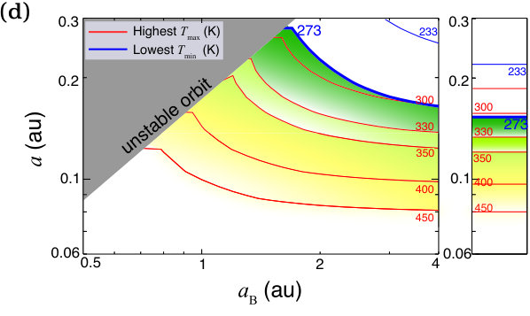 Figure 5
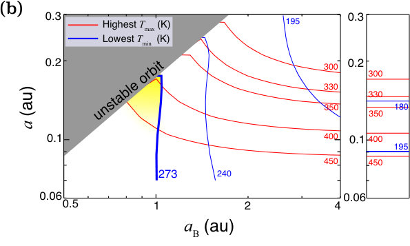 Figure 6
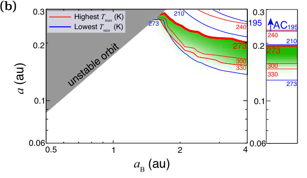 Figure 7
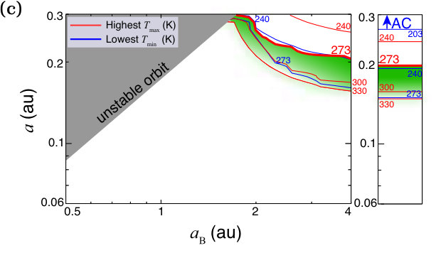 Figure 8
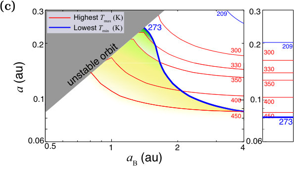 Figure 9
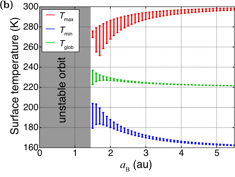 Figure 10
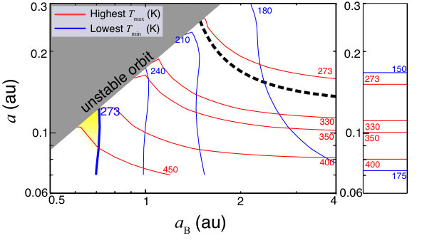 Figure 11
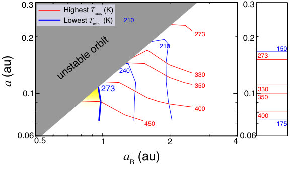 Figure 12
 Figure 13
 Figure 14
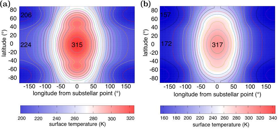 Figure 15
 Figure 16
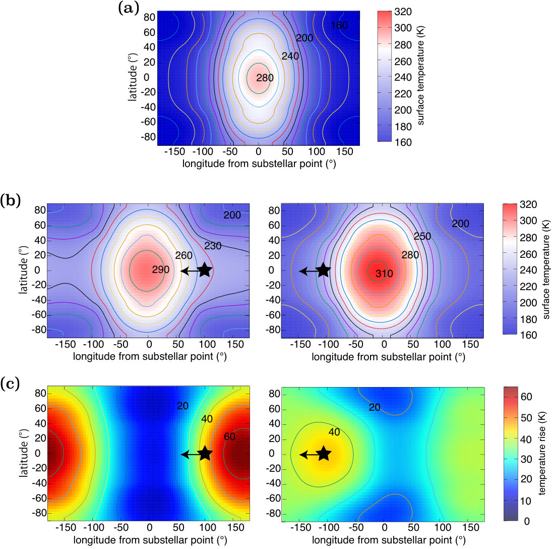 Figure 17
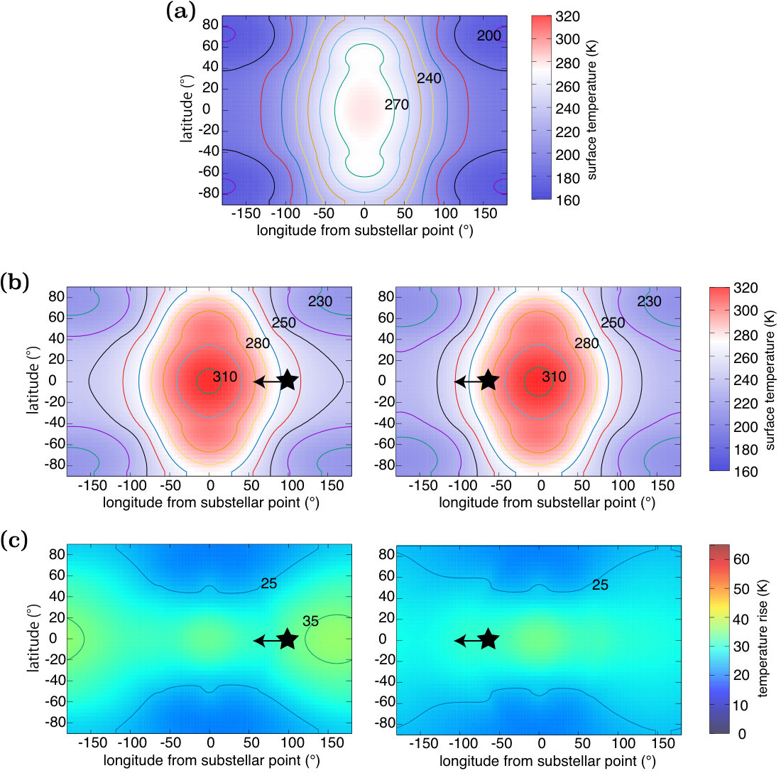 Figure 18
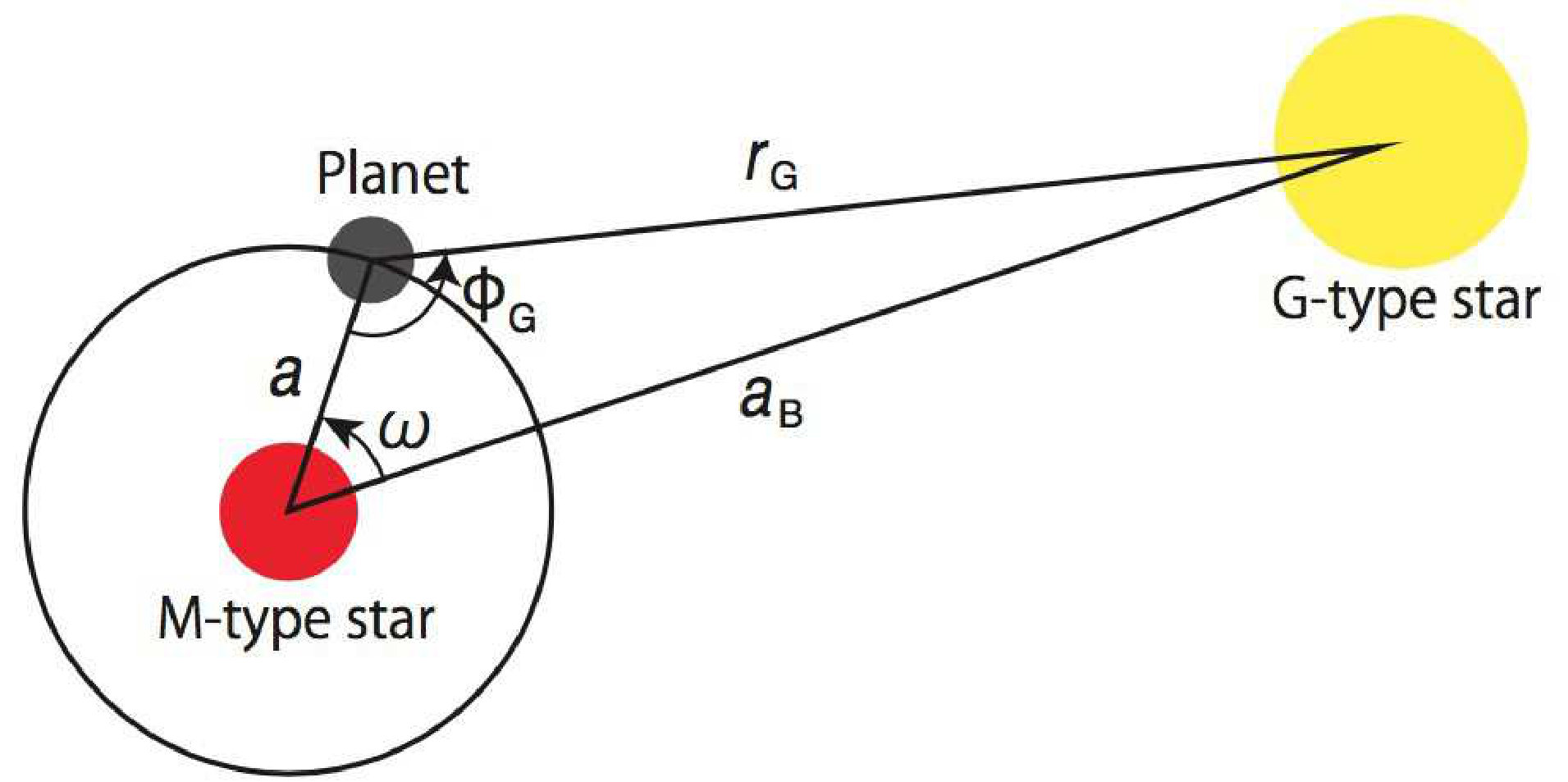 Figure 1
 Figure 20
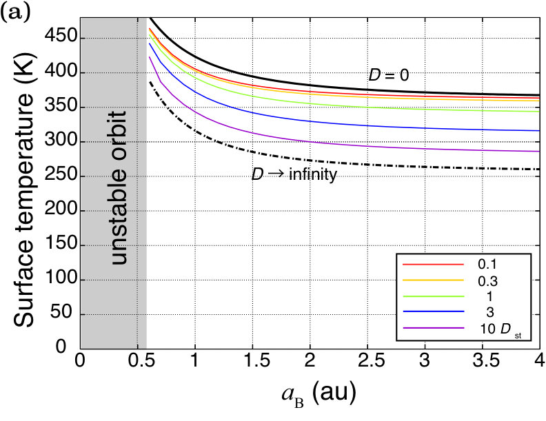 Figure 21
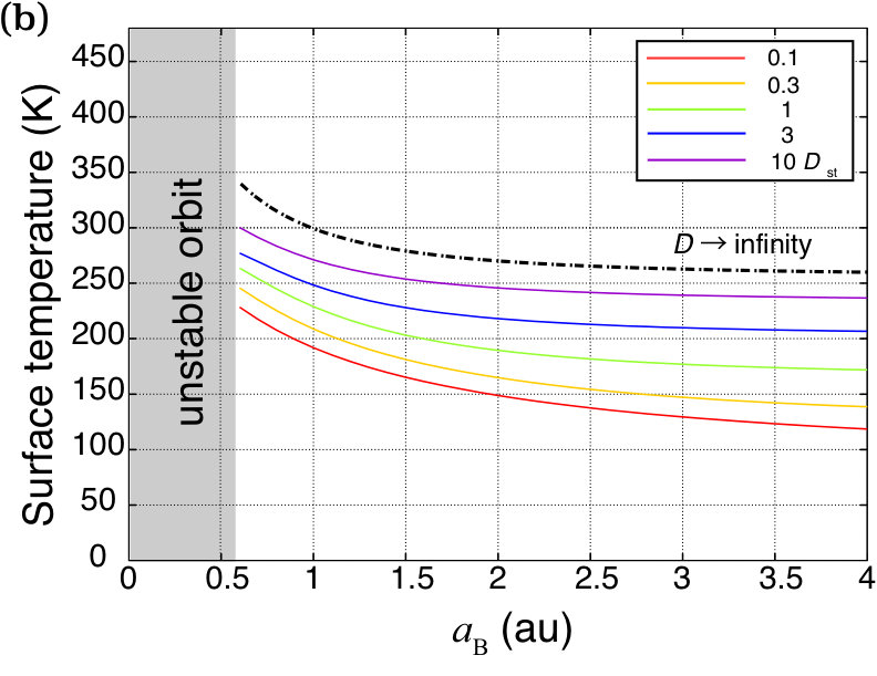 Figure 22
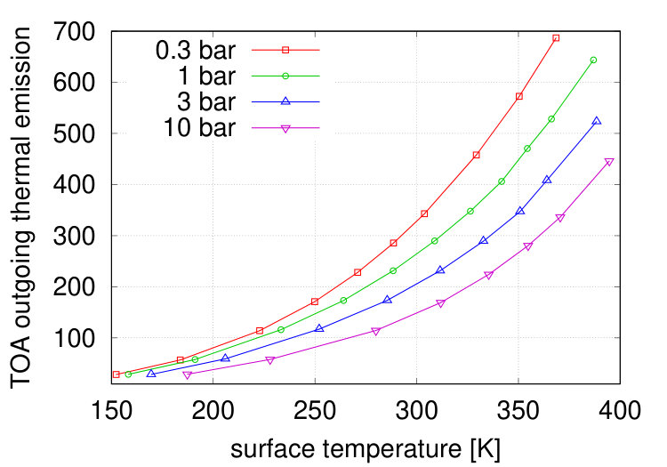 Figure 23
| Spectral Type | Luminosity [] | Mass [] | |
|---|---|---|---|
| G2V | 5778 K | 1 | 1 |
| M3V | 3300 K | 0.01 | 0.25 |
| (18) | |||||
| (19) |
| CO2 pressure | 0.3bar | 1bar | 3bar | 10bar | |
|---|---|---|---|---|---|
| [W m-2 K | |||||
| [W m-2 K | |||||
Peer Reviews
No public reviews on file for this paper yet. If you reviewed it on a platform where reviews are public (OpenReview, ICLR, NeurIPS, ICML), you can paste yours below so the community can read it here.
Videos
No videos yet. Explain this paper in a talk, walkthrough, or lecture? Add one.
Effects of a binary companion star on habitability of tidally locked planets around an M-type host star
Department of Earth and Planetary Sciences, Tokyo Institute of Technology, Ookayama, Meguro, Tokyo 152-8551, Japan
Yuka Fujii
Earth-Life Science Institute, Tokyo Institute of Technology, Ookayama, Meguro, Tokyo 152-8550, Japan
Shigeru Ida
Earth-Life Science Institute, Tokyo Institute of Technology, Ookayama, Meguro, Tokyo 152-8550, Japan
(Accepted June 12, 2019)
Abstract
Planets in the “Habitable Zones” around M-type stars are important targets for characterization in future observations. Due to tidal-locking in synchronous spin-orbit rotations, the planets tend to have a hot dayside and a cold nightside. On the cold nightside, water vapor transferred from the dayside can be frozen in (“cold trap”) or the major atmospheric constituent could also condense (“atmospheric collapse”) if the atmosphere is so thin that the heat re-distribution is not efficient, in the case of a single M-type star. Motivated by the abundance of binary star systems, we investigate the effects of irradiation from a G-type companion star on the climate of a tidally locked planet around an M-type star using the 2D energy balance model. We find that the irradiation from the G-type star is more effective at warming up the nightside of the planet than the dayside. This contributes to the prevention of the irreversible trapping of water and atmosphere on the cold nightside, broadening the parameter space where tidally locked planets can maintain surface liquid water. Tidally locked ocean planets with 0.3 bar atmospheres or land planets with bar atmospheres can realize temperate climate with surface liquid water only when they are also irradiated by a companion star with a separation of 1 - 4 au. We also demonstrate that planets with given properties can be in the Earth-like temperate climate regime or in a completely frozen state under the same total irradiation.
astrobiology — planets and satellites: atmospheres — planets and satellites: terrestrial planets — stars: binaries: general
††journal: The Astrophysical Journal††software: SOCRATES (Edwards & Slingo, 1996; Edwards, 1996)
1 Introduction
Planets in the so-called “Habitable Zones” (HZs), where liquid water can exist on the planetary surface, around M-type stars are easier to detect through radial velocity surveys owing to the smaller stellar mass and HZs closer to the star. Their small stellar size also has an advantage in transit detection of small planets. The Earth-sized planets recently discovered around the HZs, TRAPPIST-1 e, f, and g, Proxima centauri b, and LHS 1140b, orbit M-type stars. Future observations with the James Webb Space Telescope and ground-based extremely large telescopes will aim to characterize the atmospheres of these planets around M-type stars to search for habitable conditions and eventually for biosignatures.
These planets are likely to be tidally locked due to their proximity to the host stars (Kasting et al., 1993), and to have a fixed warm/hot dayside and cold nightside. Non-sunlight in the cold hemisphere poses at least two potential problems for the habitability of the planet: i) “atmospheric collapse” and ii) “cold trap” of surface water. If the local temperature on the nightside is so low that the major atmospheric constituent condenses out, the loss of the greenhouse effect and heat transport would cause further cooling, and the planet would undergo a transition into a cold state with a thin atmosphere. This phenomenon is called “atmospheric collapse” and has been considered an obstacle to habitability (e.g., Joshi et al., 1997). In addition, on the planets with a limited small amount of surface water (“land planets”), the water is transported from warmer regions to cooler ones by atmospheric circulation (Abe & Abe-Ouchi, 2005; Abe et al., 2011). In the tidally locked land planet, the dayside would be left free from water, and all of the water would be frozen on the nightside (Leconte et al., 2013). The “cold trap” of water would be irreversible unless ice flow driven by gravity or internal thermal flux is strong enough (Leconte et al., 2013; Turbet et al., 2016, 2017).
If the planet-hosting M-type star has a much brighter stellar companion such as a G-type star, it periodically irradiates the cold nightside of a tidally locked planet around the M-type star. Such a configuration may rescue HZ planets from the above-mentioned difficulties if the binary separation is appropriate: close enough for the irradiation of the companion star to affect the planetary climate, but not too close to ensure the stability of the planetary orbit. In reality, systems comprised of an M-type star and G-type star are not rare. About half of all G-type stars in the solar neighborhood have binary companions and the number distribution of their mass ratio (), , is approximately constant (Raghavan et al., 2010). In other words, a substantial fraction of G-type stars have M-type companion stars.
Circumsteller planets in binary systems like those described above are called “S-type” planets, as opposed to the circumbinary planets called “P-type” planets. More than 60 S-type exoplanets are known today. While most of them are wide binaries, a relatively close binary system such as Kepler 420 A and B, with a separation of 5.3 au has an S-type eccentric giant planet with semimajor axis 0.38 au around Kepler 420 A (Santerne et al., 2014). Although it is not easy to detect S-type planets in close binary systems, future surveys may reveal the occurrence rate of S-type planets. For example, Oshagh et al. (2017) proposed a new detection method for S-type planets in eclipsing binaries by using a correlation between the stellar radial velocities (RVs), eclipse timing variations (ETVs), and eclipse duration variations (EDVs). Whether S-type planets in close binaries are common or not is an active field of research from the viewpoint of planet formation. Circumstellar disks can exist if the disk radius is smaller than of the binary separation, and gas accretion from the circumbinary disk to the individual circumstellar disks may exist (Artymowicz & Lubow, 1994). It may be possible that the S-type planets are formed in the stable regions of these disks, although many issues remain to be studied (e.g., Thebault & Haghighipour, 2015; Dupuy et al., 2016; Gong & Ji, 2018). We leave the formation of S-type planets in relatively close binary systems for future studies.
Some previous studies (Kaltenegger & Haghighipour, 2013; Jaime et al., 2014) have considered the habitability of S-type planets, by extending the HZs of single stars obtained with 1D modeling of planetary atmospheres (e.g. Kasting et al., 1993; Kopparapu et al., 2013). Their estimates of HZs of S-type planets are based on the total irradiance the planet receives from both stars and the orbital stability condition, and did not take into account the horizontal dimension of the planetary surface. However, as we pointed out above, investigations into the habitability of planets should take into account the effects of atmospheric collapse and cold trap, and therefore the global structure of planetary surface temperature is essential. An approach to address these effects is GCM (General Circulation Model) simulations where individual physical and chemical processes including radiative transfer, atmospheric/oceanic dynamics, and phase transition of water are calculated on the three-dimensional grids; GCM simulations have been applied to tidally locked planets around single M-type stars (e.g., Turbet et al., 2016, 2017; Kopparapu et al., 2017; Fujii et al., 2017). An alternative approach is the Energy Balance Model (EBM), which finds the planetary surface temperature distribution by solving simple horizontal energy transfer across the planetary surface. While EBM greatly simplifies or ignores the individual physical and chemical processes that control the energy transfer, EBMs have been useful to study basic climatological properties of exoplanets (Spiegel et al., 2009, 2010; Checlair et al., 2017).
In this paper, we study the effects of irradiation from a G-type companion star on the condition of habitability of tidally locked planets around an M-type star (S-type planets), taking into account the effects of atmospheric collapse and cold trap. In order to gain insights into the first-order behavior of the planetary climate exploring a broad parameter space, we use two-dimensional EBM calculations (e.g. North, 1975) rather than complex and computationally expensive GCM simulations. The planet is assumed to be either fully covered with water (“ocean-covered”) or to have a limited amount of water with most of the surface being bare (“land-covered”), and its atmosphere is either Earth-like or CO2-dominated. For each class of planets, we estimate the binary separation that allows for the presence of liquid water on their surfaces.
In Section 2, we describe our assumptions on the binary system, the energy balance model used to calculate the the planetary surface temperature distribution,and our criteria for atmospheric collapse and the cold trap based on the planetary surface temperature distribution. In Section 3, we demonstrate the surface temperature maps with and without a G-type companion star, and analyze the behavior of temperature on ocean- or land-covered planets by changing binary separations. Finally, we present the orbital region where planets of different types can maintain temperate climate and compare them to the case of a planet around a single M-type star without a companion star. We discuss parameters that would affect our results and observability of the planets we focus on in Section 4, and summarize our findings in Section 5.
2 Model
In section 2.1, we explain the settings of the binary stars and the S-type planet that we simulate. In section 2.2, we describe the two-dimensional EBM for the planet and the input parameters. Section 2.3 introduces our criteria for the atmospheric collapse and cold trap.
2.1 Assumed System Architecture
We consider binary systems composed of a G2V and an M3V main-sequence star whose basic parameters are summarized in Table 1: the G-type star has the luminosity and the mass , and the M-type star has and , consistent with the mass-luminosity relation of M-type stars (e.g., Boyajian et al., 2012). We change the binary separation between the G-type star and the M-type star from 0.1 au to 5.5 au by 0.1 au.
In most of the calculations in this paper, we assume that the binary eccentricity, , is zero for simplicity. Observations show that the median eccentricity for binary periods of 10 - 1000 days is (Duquennoy & Mayor, 1991). We will discuss the case of in Section 3.3.4. In addition, we set the binary inclination relative to the planetary orbital plane as for simplicity. The discussion on the effects of non-zero is left for future work.
We assume that the M-type star is orbited by a rocky planet. The mass and radius of the planet are set at Earth’s values. The semimajor axis of the planet is changed within the range of where is the maximum semimajor axis for the planetary orbit not to be destabilized by the secular perturbations from the G-type star. We use the fitting formula by Pichardo et al. (2005):
[TABLE]
where is the binary separation, and and are the masses of the M-type and G-type stars. For ,
[TABLE]
We assume a circular planetary orbit () and zero obliquity because of the tidal dissipation in the planet. If the binary eccentricity is not equal to 0, the planetary eccentricity may oscillate. Within the limits of weak tidal dissipation, the maximum value of the oscillating eccentricity is (e.g., Murray & Dermott, 1998),
[TABLE]
For , . Even in the case of , , which may be negligible.
We postulate that a planet is tidally locked in a 1:1 spin-orbit state. The tidal-locking limit for a M3V star is estimated to be 0.3 au, and we confine our study to this range, consistent with the postulation. As we will see later, the orbital region where planets have temperate climate are mostly within this limit.
2.2 Energy Balance Model
We use an Energy Balance Model (EBM) to study a time-dependent temperature distribution of a tidally locked rocky planet orbiting an M-type star and having a G-type companion star.
An EBM has been widely used to study the climate of the Earth (e.g. North, 1975) and Mars (e.g. James & North, 1982). EBM solves the planetary surface temperature distribution taking into account the local net radiation flux and the horizontal heat transport; detailed processes including the vertical profile of the atmosphere and phase transition of water are not explicitly solved. This is in contrast to General Circulation Models (GCMs) where these processes are parameterized and solved at each 3-dimensional (2 for horizontal, 1 for vertical) grid cell. Because of such simplification, the results from EBM may not be quantitatively accurate. However, EBM is useful in revealing the planetary climate’s global trend in response to external forces, and EBM calculations are analytically more tractable. A much broader parameter space can be surveyed and it is easier to reveal intrinsic physics with EBM, if the model is properly calibrated by the GCM simulations. We will calibrate our EBM calculations with the results of GCM simulations for tidally locked planets around single M-type stars by Turbet et al. (2016, 2017).
In order to take into account not only the static irradiation from the M-type star, but also the periodic irradiation from the G-type companion star, we adopt a time-dependent two-dimensional (latitude and longitude ) EBM, based on North (1975). We use grids. The energy balance equation is
[TABLE]
where is the planetary surface temperature, is time, and is the heat capacity of the surface, is heating by the host star and the companion stars, is thermal outgoing radiation, and is the diffusion coefficient. The heating, , is a sum of the time-independent incoming irradiation flux from the M-type star, , and the time-dependent (periodic) one from the G-type stars, ,
[TABLE]
where and are the irradiance by the M-type star and the G-type companion star, respectively, and and are corresponding albedos. With the input parameters described below, Equation (4) is solved under the boundary condition with no heat transport at the poles for and the periodic boundary condition for . The numerical calculations continue running until an equilibrium periodical cycle is achieved.
The heat capacity (), albedo (), outgoing thermal flux (), and diffusion coefficient are determined as described below, depending on the surface and atmospheric conditions. In this paper, we consider the combinations of two surface types and two atmospheric types. For the surface environment, we consider two limiting cases: rocky planets wholly covered with ocean, “ocean planets, and dry planets with a mostly bare surface but with a small amount of water, “land planets.” For the atmospheric condition, either an Earth-like atmosphere (composed of N2 and O2 with 376 ppm CO2) or CO2-dominated 0.3-10 bar atmosphere is assumed. In summary, we consider the following four types:
- (OE)
ocean planets with Earth-like atmospheres with 1 bar mixture of N2 and O2 with 376 ppm CO2 with varying amount of water vapor,
- (OC)
ocean planets with CO2-dominated atmospheres of and 2 bar, with varying amount of water vapor,
- (LE)
land planets with Earth-like dry atmospheres (same as (OE) but without water vapor), and
- (LC)
land planets with pure CO2 atmospheres of , and 10 bar.
From a point of view of the planetary formation, land planets are potentially important targets in future observations searching for habitable worlds, especially around M-type stars. Unlike G-type stars, M-type stars experience a prolonged pre-main-sequence stage with an order of magnitude higher luminosity than that in their main-sequence stage. During this stage, planets that currently reside in the HZ would have been exposed to extreme irradiation and would have lost a significant amount of the water it originally had (if any) (Ramirez & Kaltenegger, 2014; Tian & Ida, 2015; Luger & Barnes, 2015). Thus, the substantial number of an planets in the HZ of an M-type star may be desert planets (Tian & Ida, 2015), and later delivery of a small amount of water will then make them land planets.
2.2.1 Heat Capacity
The values for for ocean and land planets are adopted from the Earth’s values for ocean and land, respectively, which are and (Pollard, 1983). Over sea-ice, takes twice value of for K. The values for other parameters will be discussed in Section 2.2.2, 2.2.4, and 2.2.5 below.
2.2.2 Irradiation
The irradiance from the two stars on the location of the planetary surface is given by
[TABLE]
where is the distance between the planet and the G-type star (see Figure 1), given by
[TABLE]
is the angle between the direction to the planet and that to the G-type star from the M-type star,
[TABLE]
and and are Keplerian frequencies of the planet and G-type star, respectively. The longitude of the substellar point of the G-type star is given by
[TABLE]
As Eq. (9) shows, both and oscillate with the synodic period between the planet and the G-type star relative to the M-type star, causing the periodic change in the insolation pattern of the planet.
2.2.3 Albedo
The albedos in Eq. (5), and , depend on the planetary surface and atmospheric composition and pressure. The values we used are summarized in Table 2.2.6 and the assumptions are detailed below.
The albedo of a cloud-free atmosphere with an underlying surface is generally given by the following combination of albedo of the atmosphere () and that of the bare surface () as
[TABLE]
In practice, is the average of wavelength-dependent scattering efficiency weighted by the spectrum of M-type or G-type stars. The prescription of for different types of atmospheres will be detailed below.
The surface albedo, , is assumed to be 0.07 for liquid ocean surface and 0.2 for the surface of land planets, regardless of the irradiance spectrum. For ocean planets, we also take account of the change of surface albedo due to ocean freezing; when the surface temperature is below 273 K, we assume that the ocean instantaneously freezes and replace the surface albedo by that of ice/snow, which is 0.3 and 0.55 with respect to the spectrum of the M-type star and the G-type star, respectively. The difference in sea ice albedo is due to the redder spectrum of the M-type star where the ice/snow albedo is lower.
However, the albedo of ocean planets may be better characterized by water clouds. The GCM simulations for tidally locked ocean planets show that the region covered by the liquid water on the dayside is likely to be covered by optically thick water clouds due to convection (e.g. Yang et al., 2013), while the nightside or frozen surface tends to be free from thick clouds. In order to take it into account, we modified the albedo for the unfrozen area on the dayside of ocean planets to 0.4.
We summarize our prescriptions of the albedo for each atmospheric condition below (For the detailed values, see Table 2.2.6).
Ocean planets, Dayside to the M-type star radiation and above 273 K:
We adopt the cloud-covered albedo 0.4, which is independent of atmospheric composition and pressure. 2. 2.
Ocean planets, Otherwise:
We adopt the cloud-free albedo given by Eq. (11).
The surface albedo, , depends on the surface temperature. Above 273 K, . Below 273 K, it is 0.3 and 0.55 for the irradiation of the M-type star and the G-type star, respectively.
The atmospheric albedo with respect to the M-type star spectrum, which is determined by the combination of Rayleigh scattering and atmospheric absorption, is obtained by performing the radiative transfer calculation for each type of atmosphere using SOCRATES (Edwards & Slingo, 1996; Edwards, 1996) described in the appendix A. A saturated atmosphere with surface temperature of 273 K is assumed. Precisely speaking, depends on the surface temperature due to the change in the column density of water vapor. We also calculated the albedo with the lower surface temperature (200K) and found that deviation in terms of the value of is within %. The atmospheric albedo with respect to the G-type star are calculated using analytic formula for different types of atmospheres.
type OE
The albedo for M-type star’s irradiation is calculated using SOCRATES assuming an 1 bar N2-dominated atmosphere composed of 21% O2, and 300 ppm CO2. The albedo for G-type star’s irradiation is calculated by the single-scattering approximation with Earth’s Rayleigh scattering optical depth by Young (1980), as described in Fujii et al. (2010).
type OC
The albedo for M-type star’s irradiation is calculated using SOCRATES assuming a pure CO2 atmosphere. The albedo for G-type star’s irradiation is determined based on the analytical expression by Yokohata et al. (2002) which considered the Martian atmosphere, with a modification due to the difference in gravity (we assume Earth’s value for the gravity, , in this paper): with bar. 3. 3.
Land planets:
We adopt the cloud-free albedo given by Eq. (11) with the surface albedo is set at 0.2 (Turbet et al., 2016). The atmospheric albedo for different types are given as follows:
type LE
The atmospheric albedo is obtained by the same calculation as the the cloud-free region of type OE except that the Rayleigh scattering efficiency is replaced by that of dry air.
type LC
The atmospheric albedo is obtained by the radiative transfer calculation with SOCRATES (see Appendix A).
2.2.4 Thermal emission
For land planets, the radiation flux from the top of the planetary atmosphere in Equation (4) is given in a form of a modified black-body radiation as
[TABLE]
where is a fitting parameter as a function of CO2 partial pressure111Precisely speaking, also depends weakly on the surface temperature (). In this paper, however, we ignore the dependence for simplicity. (Table 2.2.6). With the Earth-like atmosphere, the parameter is approximated by the Stefan-Boltzmann constant in this paper. With a CO2 atmosphere, is obtained by our 1D radiative-convective equilibrium calculation. The procedure is detailed in Appendix A.
For ocean planets, at Earth-like temperatures, is approximately linear to the temperature due to the strong greenhouse effect of water vapor (e.g. Koll & Cronin, 2018, and the references therein). Imposing its asymptotic approach to Eq.(12) at low temperature, the functional form of of ocean planets can may written as (Spiegel et al., 2008),
[TABLE]
where the coefficient of Eq. (14) is adopted from Spiegel et al. (2008). Comparing Eq. (13) to the linear expression of Caldeira & Kasting (1992) which is valid for the range of bar CO 2 bar and 194K 303K, the discrepancy is 10 % for the most of this range except below 200K. Since 3 bar and 10 bar runs are out of this range, we did not calculate these runs for ocean planets.
However, is also affected by clouds that we assumed for albedo (see section 2.2.3), as cloud cover tends to reduce the top-of-atmosphere outgoing thermal emission. In this paper, we assume the constant cloud-top temperature K as a crude approximation referring to the fixed anvil temperature theory (Hartmann & Larson, 2002) and some GCM results for tidally-locked planets (Yang & Abbot, 2014). Thus, the thermal emission for the overcast region of the dayside is modified as follows:
[TABLE]
2.2.5 Diffusion term
The thermal diffusion due to the atmospheric and the oceanic flows can be divided into latitudinal and the longitudinal components:
[TABLE]
where and are latitudinal and longitudinal diffusion coefficients, respectively. On the Earth, and their values on the ocean are twice as large as those on the land, which reflects the substantial contribution of oceanic flow to the heat transport. For ocean and land planets with Earth-like atmospheres, the values for are taken from the Earth’s values for ocean and land, respectively (Pollard, 1983), while is adjusted for the characteristics of tidally locked planets as follows: GCM calculations for the tidally locked planets (Turbet et al., 2016, 2017; Kopparapu et al., 2017) showed characteristic patterns of atmospheric circulation with the coldest regions at high latitudes on the nightside (off the polar regions) associated with the zonal flow developed near the equator. Corresponding to these patterns, for ocean (land) planets, we set to be 0.03 (0.02) times larger than the Earth’s value at degrees and to be 1.5 (1.0) times larger than the Earth’s value otherwise.
In order to obtain the values for and for planets with CO2-dominated atmospheres of various surface pressure, we scale the Earth’s values assuming the following dependence:
[TABLE]
where is atmospheric pressure, , and is the heat capacity of the atmosphere. We note that the potential dependence on other parameters is ignored here. In reality, atmospheric and oceanic flows that control and would be affected by the spin rate, and irradiation patterns among others. For tidally-locked planets, this means and should also depend on the planetary semi-major axis, . The exact dependence of these parameters would be nonlinear, however, and would require the GCM computations. We will discuss this in Section 4.2.
2.2.6 Validation
In order to test the validity of our model and parameter setting, we calculated the temperature distribution of Proxima Centauri b, an Earth-size planet at au around a single M-type host star with and . Figure 2 shows our result of the 2D distribution of surface temperature for the land and ocean planets with and , where is the solar irradiation flux at the substellar point, calculated by and of the Proxima Centauri system. The values of the maximum and minimum and their locations and the overall distribution obtained by our model agree with the previous GCM results for the planet (Figs. 3 and 6, Turbet et al., 2016).
The reference list from the paper itself. Each links out to its DOI / PubMed record.
- 1Abe & Abe-Ouchi (2005) Abe, Y., & Abe-Ouchi, A. 2005, AGU Fall Meeting Abstracts, P 51D
- 2Abe et al. (2011) Abe, Y., Abe-Ouchi, A., Sleep, N. H., & Zahnle, K. J. 2011, Astrobiology, 11, 443
- 3Allard et al. (2012) Allard, F., Homeier, D., & Freytag, B. 2012, Philosophical Transactions of the Royal Society of London Series A, 370, 2765
- 4Amundsen et al. (2017) Amundsen, D. S., Tremblin, P., Manners, J., Baraffe, I., & Mayne, N. J. 2017, A&A, 598, A 97
- 5Amundsen et al. (2016) Amundsen, D. S., Mayne, N. J., Baraffe, I., et al. 2016, A&A, 595, A 36
- 6Artymowicz & Lubow (1994) Artymowicz, P., & Lubow, S. H. 1994, Ap J, 421, 651
- 7Baranov et al. (2004) Baranov, Y. I., Lafferty, W. J., & Fraser, G. T. 2004, Journal of Molecular Spectroscopy, 228, 432
- 8Bideau-Mehu et al. (1973) Bideau-Mehu, A., Guern, Y., Abjean, R., & Johannin-Gilles, A. 1973, Optics Communications, 9, 432