TL;DR
This paper introduces two robust linear domain decomposition algorithms for simulating non-linear fracture flow in porous media, utilizing the L-scheme for linearization and multiscale flux basis for computational efficiency, with proven stability and convergence.
Contribution
The paper develops two new algorithms, MoLDD and ItLDD, that efficiently handle non-linear fracture flow problems using linearization and precomputed flux bases, advancing computational methods in this field.
Findings
Algorithms are stable and convergent under optimized parameters.
Extensive numerical tests confirm theoretical predictions.
Pre-computed flux basis reduces computational complexity.
Abstract
In this work, we consider compressible single-phase flow problems in a porous media containing a fracture. In the latter, a non-linear pressure-velocity relation is prescribed. Using a non-overlapping domain decomposition procedure, we reformulate the global problem into a non-linear interface problem. We then introduce two new algorithms that are able to efficiently handle the non-linearity and the coupling between the fracture and the matrix, both based on linearization by the so-called L-scheme. The first algorithm, named MoLDD, uses the L-scheme to resolve the non-linearity, requiring at each iteration to solve the dimensional coupling via a domain decomposition approach. The second algorithm, called ItLDD, uses a sequential approach in which the dimensional coupling is part of the linearization iterations. For both algorithms, the computations are reduced only to the fracture by…
Click any figure to enlarge with its caption.
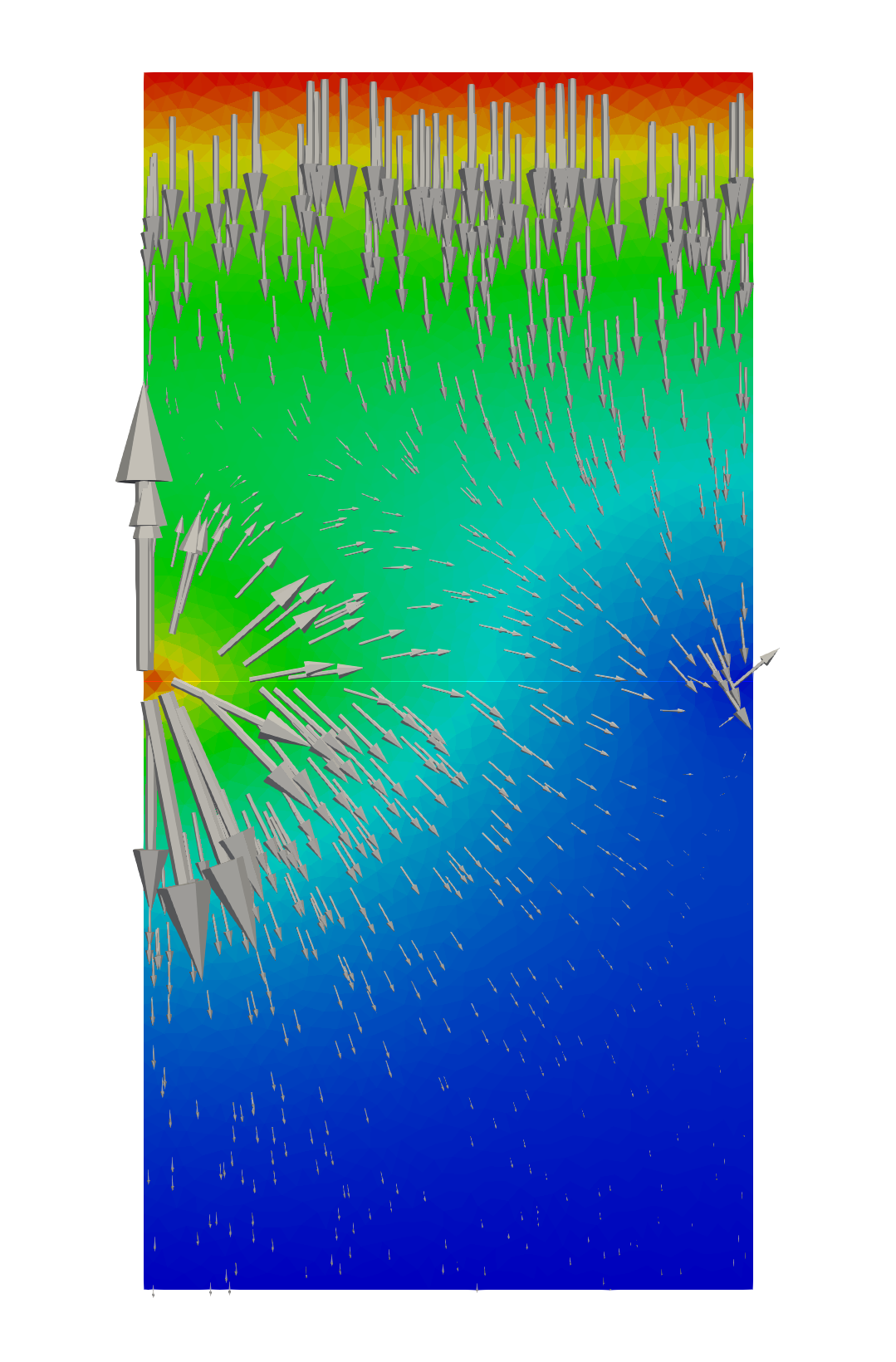 Figure 1
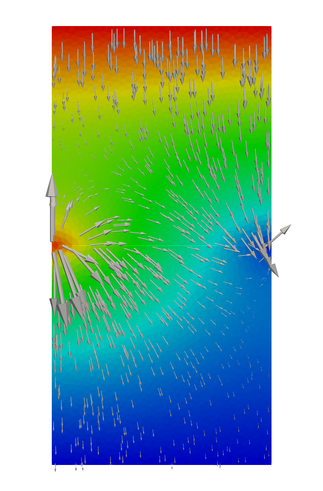 Figure 2
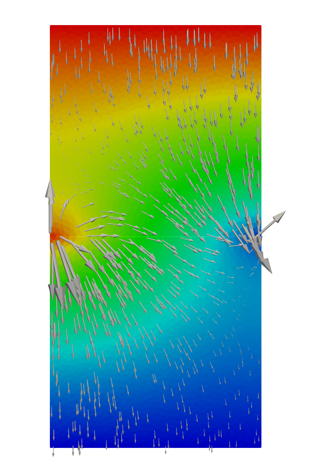 Figure 3
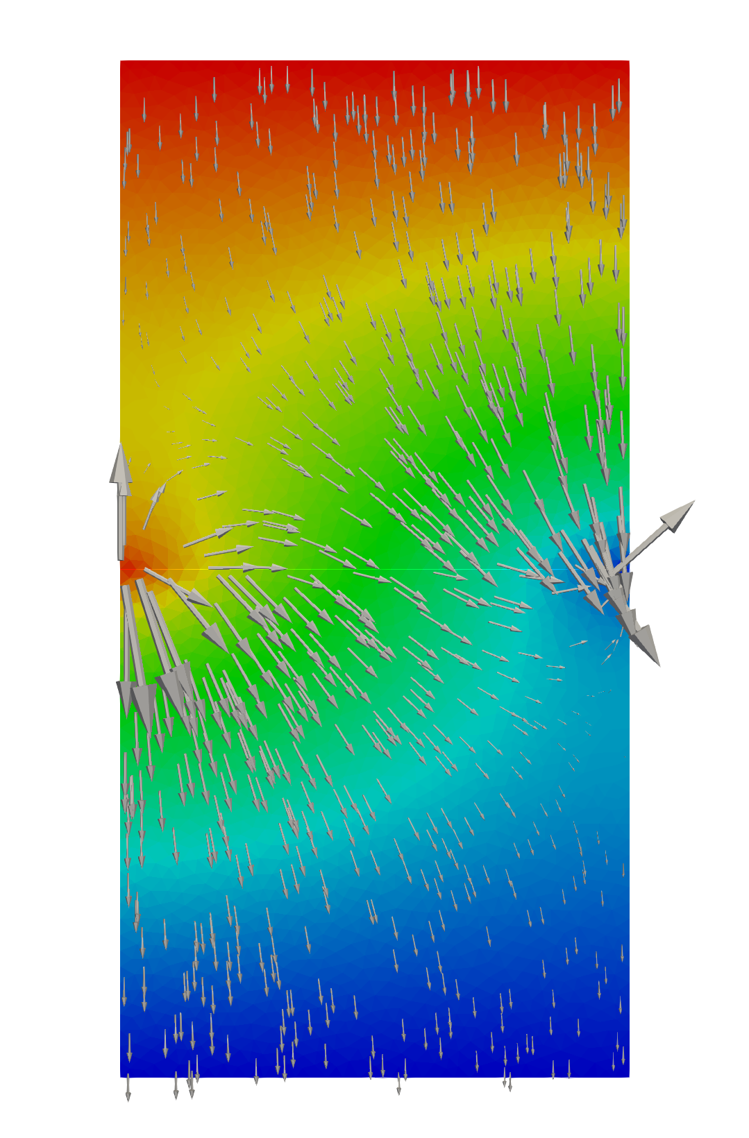 Figure 4
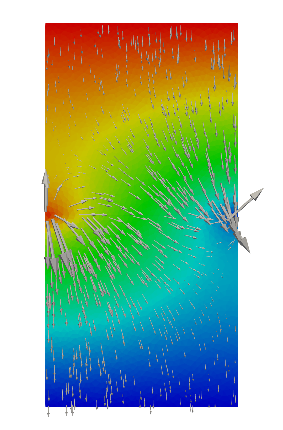 Figure 5
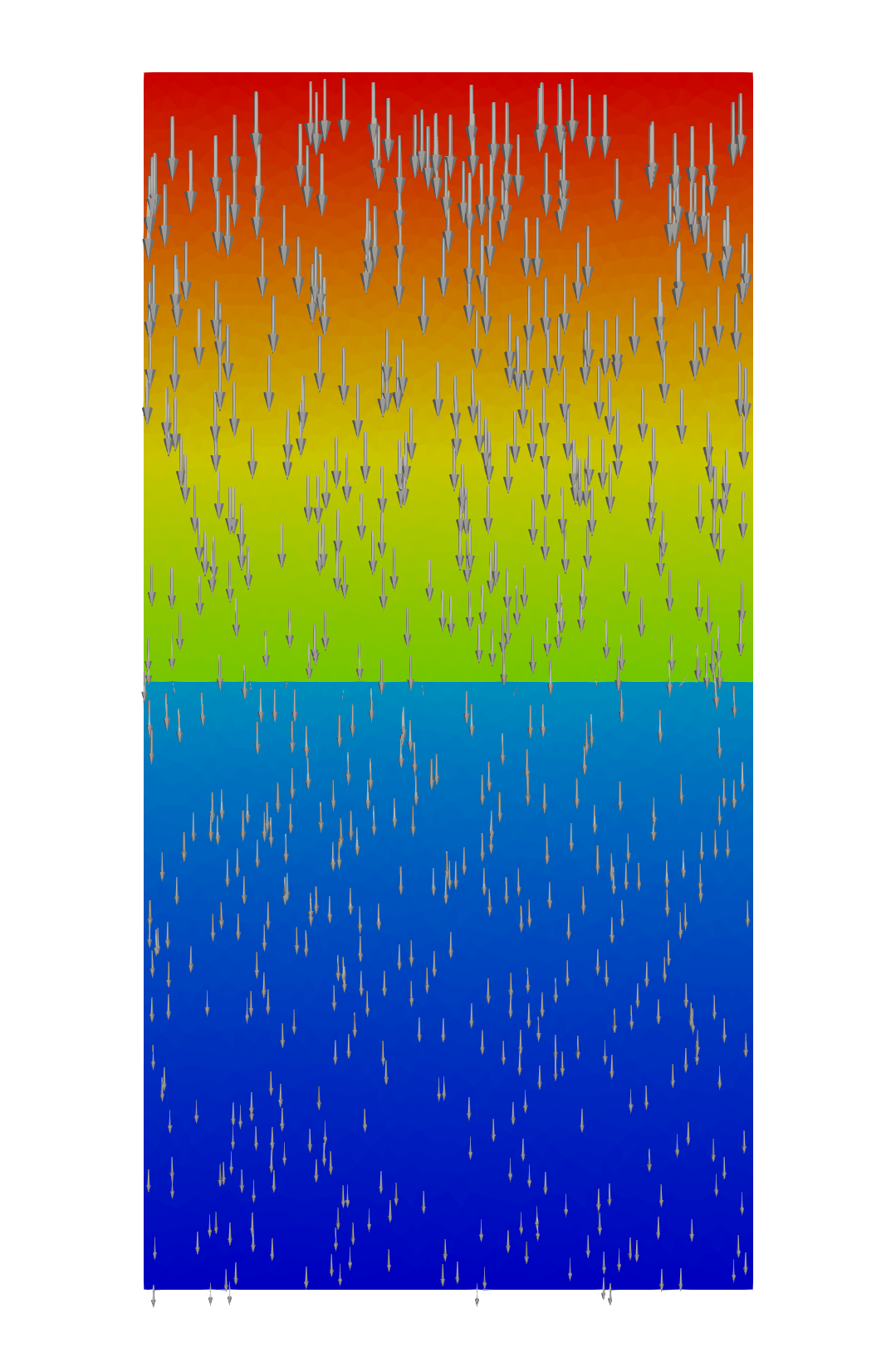 Figure 6
 Figure 7
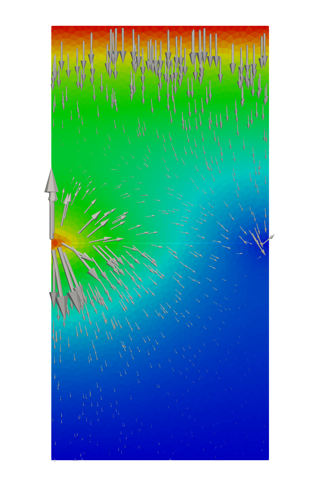 Figure 8
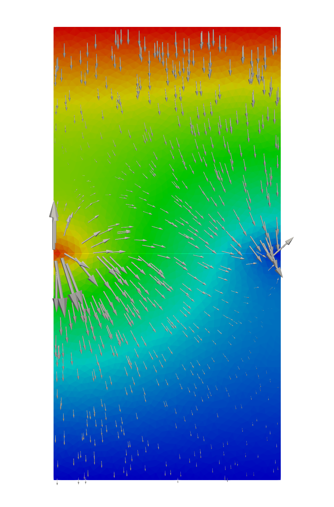 Figure 9
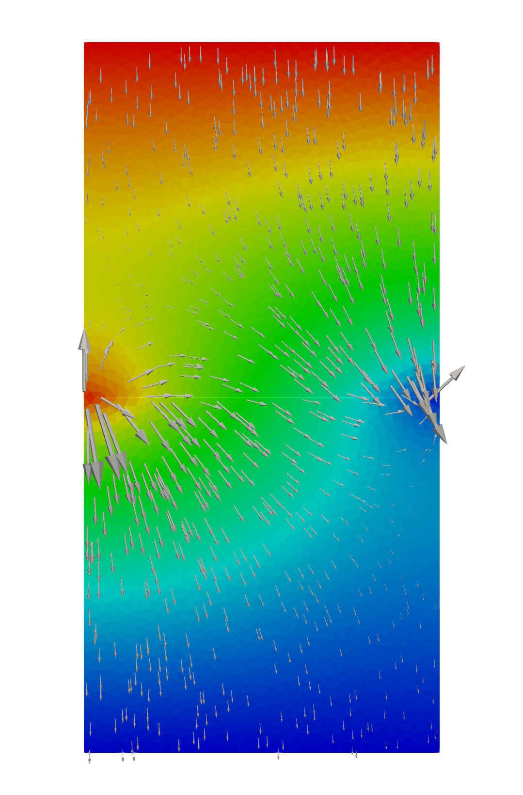 Figure 10
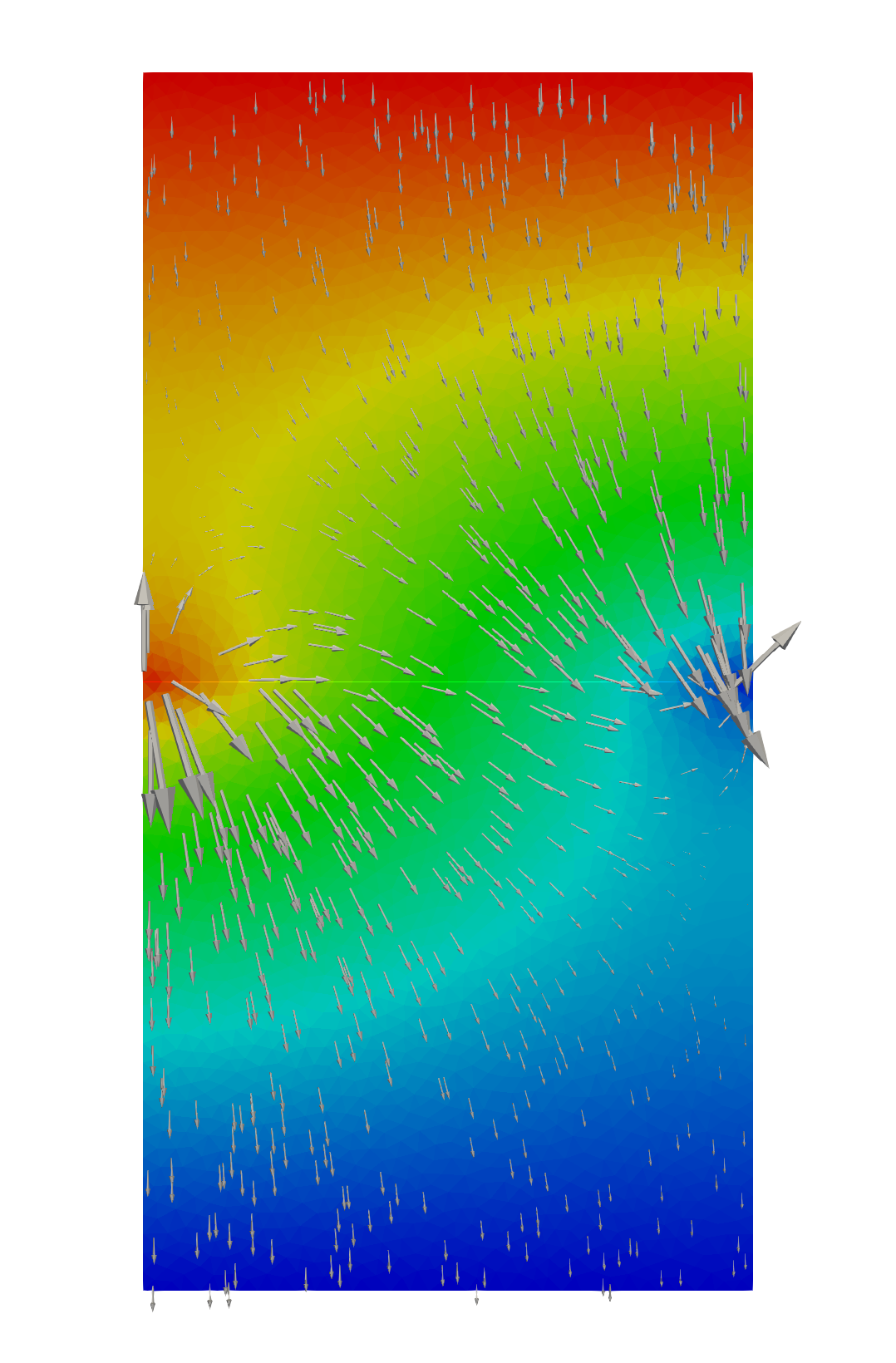 Figure 11
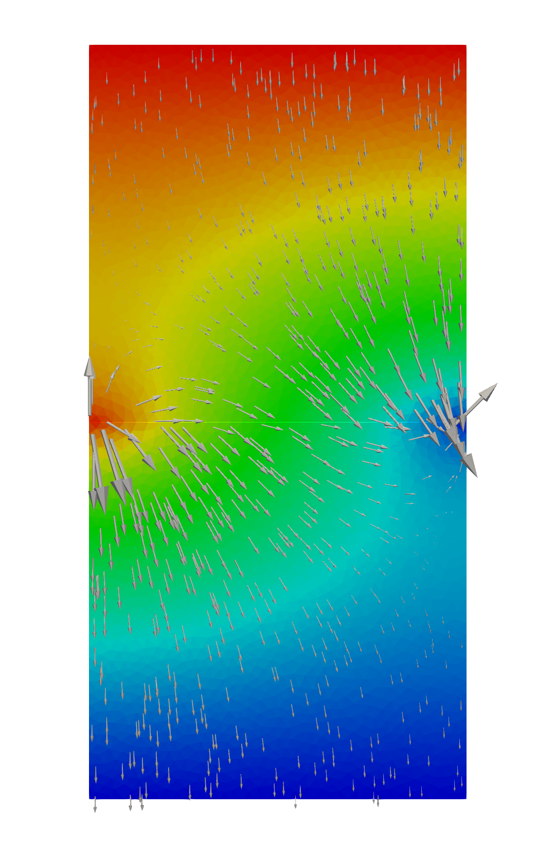 Figure 12
 Figure 13
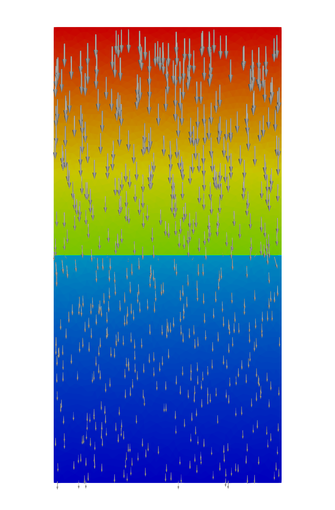 Figure 14
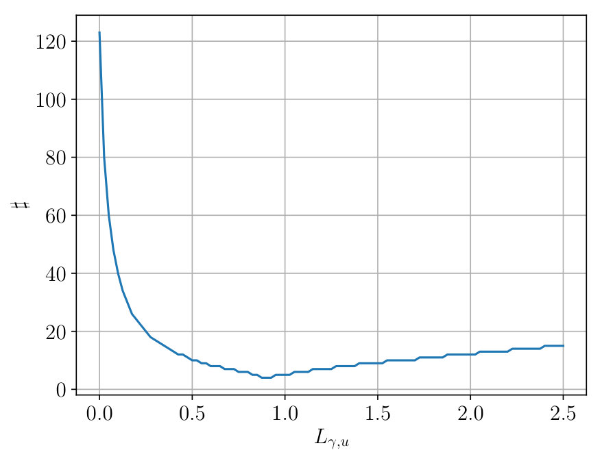 Figure 15
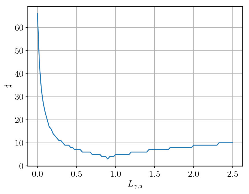 Figure 16
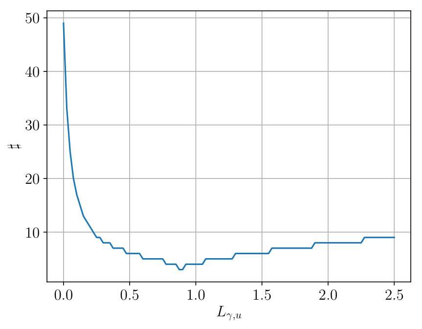 Figure 17
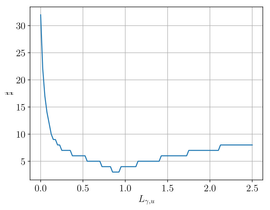 Figure 18
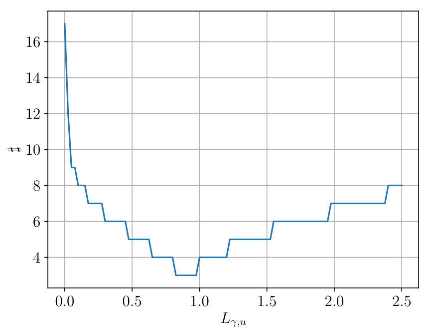 Figure 19
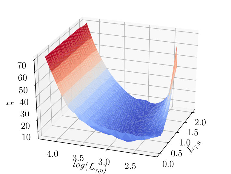 Figure 20
 Figure 21
 Figure 22
 Figure 23
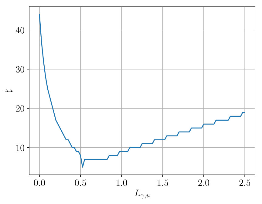 Figure 24
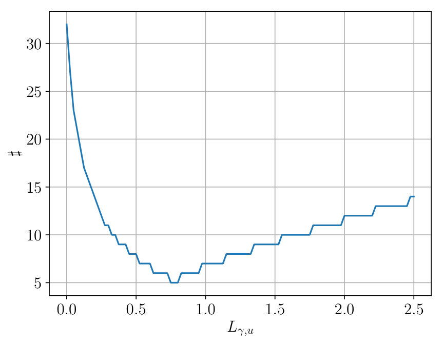 Figure 25
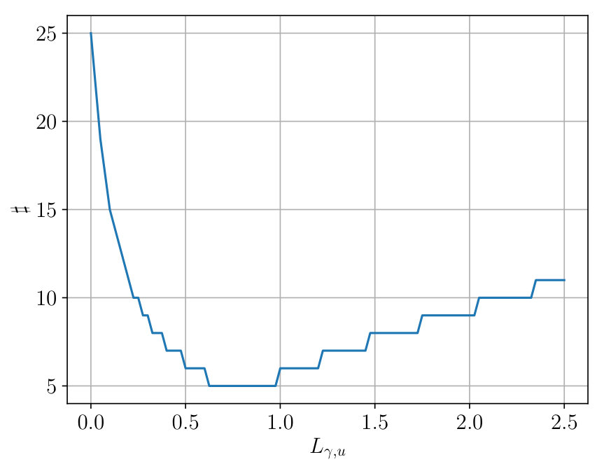 Figure 26
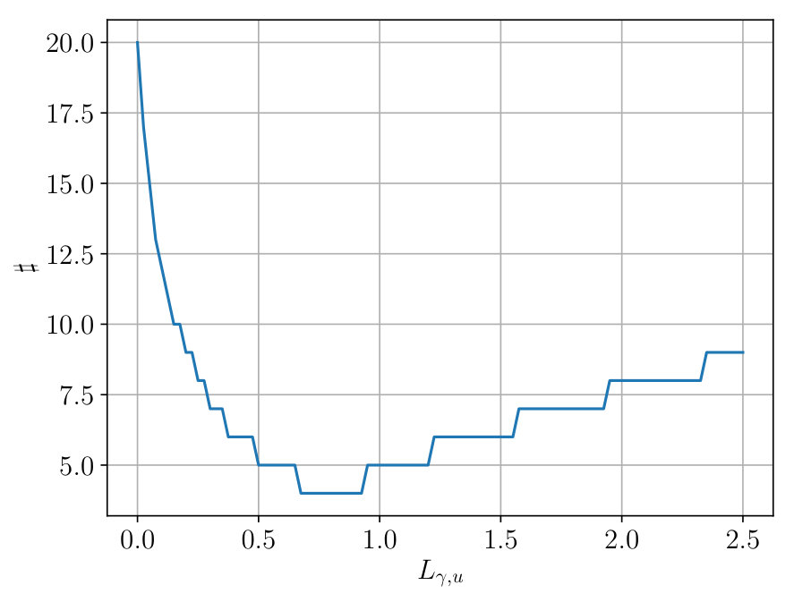 Figure 27
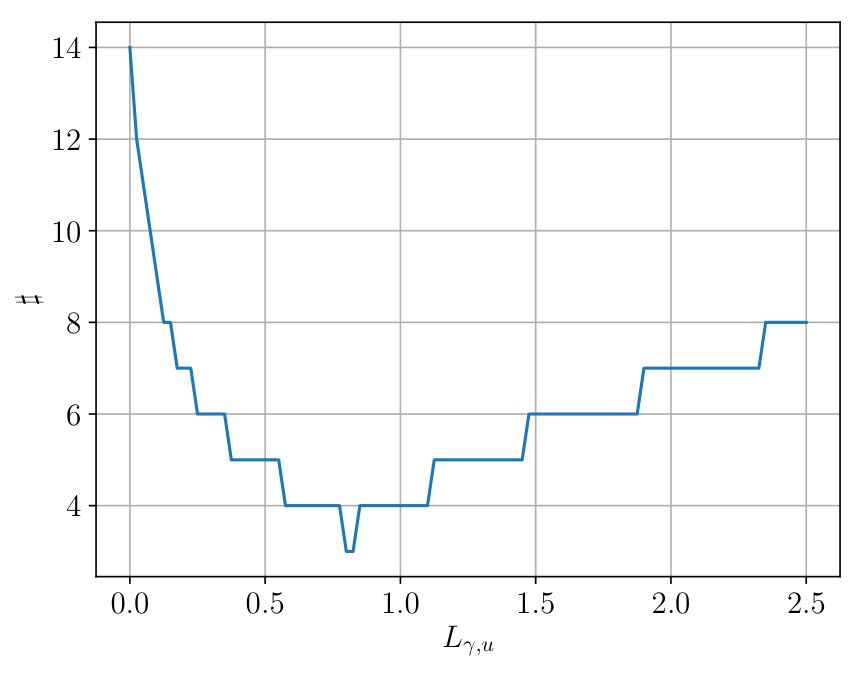 Figure 28
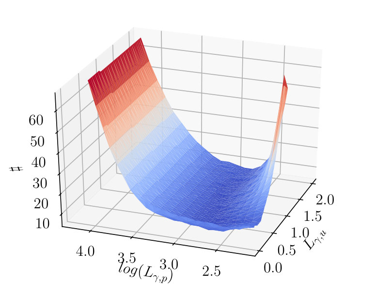 Figure 29
 Figure 30
 Figure 31
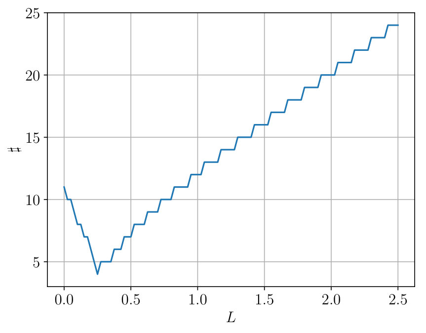 Figure 32
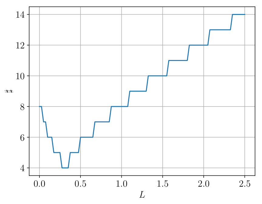 Figure 33
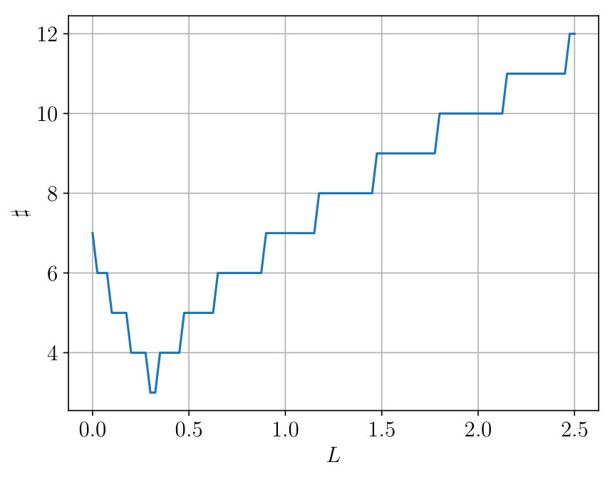 Figure 34
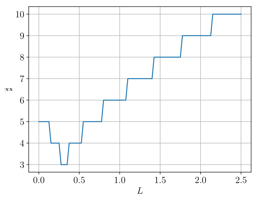 Figure 35
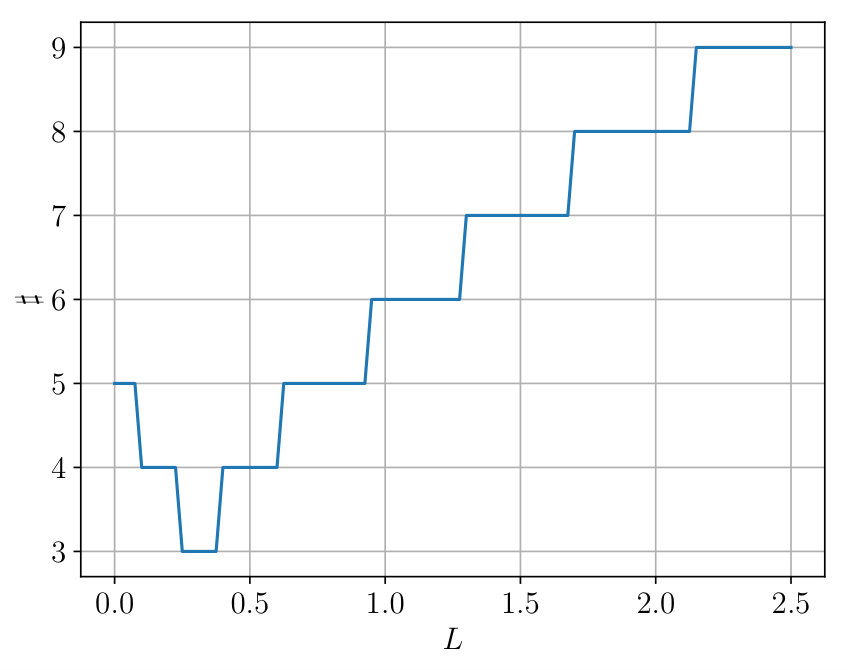 Figure 36
| 1 | 2 | 3 | 4 | 5 | |
|---|---|---|---|---|---|
| 17 | 12 | 11 | 10 | 9 | |
| 17 | 11 | 10 | 9 | 8 | |
| 17 | 11 | 10 | 9 | 8 |
| 1 | 2 | 3 | 4 | 5 | |
|---|---|---|---|---|---|
| 0.1 | 17 | 9 | 8 | 7 | 7 |
| 1 | 17 | 9 | 8 | 7 | 7 |
| 100 | 9 | 8 | 7 | 6 | 5 |
| 1 | 2 | 3 | 4 | 5 | |
|---|---|---|---|---|---|
| 8 | 3 | 3 | 3 | 3 | 2 |
| 16 | 3 | 3 | 3 | 3 | 2 |
| 64 | 3 | 3 | 3 | 3 | 2 |
| 1 | 2 | 3 | 4 | 5 | |
|---|---|---|---|---|---|
| 0.1 | 15 | 11 | 10 | 9 | 8 |
| 1 | 10 | 9 | 8 | 8 | 8 |
| 2.5 | 30 | 19 | 16 | 14 | 12 |
Peer Reviews
No public reviews on file for this paper yet. If you reviewed it on a platform where reviews are public (OpenReview, ICLR, NeurIPS, ICML), you can paste yours below so the community can read it here.
Code & Models
Videos
No videos yet. Explain this paper in a talk, walkthrough, or lecture? Add one.
Robust linear domain decomposition schemes for
reduced non-linear fracture flow models
Elyes Ahmed222Department of Mathematics, University of Bergen, P. O. Box 7800, N-5020 Bergen, Norway. [email protected], [email protected], [email protected], [email protected], 444SINTEF Digital, Mathematics and Cybernetics, Oslo, Norway (current address). [email protected],
Alessio Fumagalli111Department of Mathematics, Politecnico di Milano, piazza Leonardo da Vinci 32, 20133 Milan, Italy. [email protected].
Ana Budiša222Department of Mathematics, University of Bergen, P. O. Box 7800, N-5020 Bergen, Norway. [email protected], [email protected], [email protected], [email protected],
Eirik Keilegavlen222Department of Mathematics, University of Bergen, P. O. Box 7800, N-5020 Bergen, Norway. [email protected], [email protected], [email protected], [email protected],
Jan M. Nordbotten222Department of Mathematics, University of Bergen, P. O. Box 7800, N-5020 Bergen, Norway. [email protected], [email protected], [email protected], [email protected],
Florin A. Radu222Department of Mathematics, University of Bergen, P. O. Box 7800, N-5020 Bergen, Norway. [email protected], [email protected], [email protected], [email protected],
Abstract
In this work, we consider compressible single-phase flow problems in a porous media containing a fracture. In the latter, a non-linear pressure-velocity relation is prescribed. Using a non-overlapping domain decomposition procedure, we reformulate the global problem into a non-linear interface problem. We then introduce two algorithms that are able to efficiently handle the non-linearity and the coupling between the fracture and matrix, both based on linearization by the so-called L-scheme. The first algorithm, named MoLDD, uses the L-scheme for the non-linearity, requiring at each iteration to solve the dimensional coupling via a domain decomposition approach. The second algorithm, called ItLDD, uses a sequential approach in which the dimensional coupling is part of the linearization iterations. For both algorithms, the computations are reduced only to the fracture by pre-computing, in an offline phase, a multiscale flux basis (the linear Robin-to-Neumann co-dimensional map), that represent the flux exchange between the fracture and the matrix. We present extensive theoretical findings. The stability and the convergence of both schemes are obtained, where user-given parameters are optimized to minimise the number of iterations. Examples on two important fracture models are computed with the library PorePy and agree with the developed theory.
Key words: Porous medium; reduced fracture models; generalized Forchheimer’s laws; mortar mixed finite element; multiscale flux basis; non-linear interface problem; non-overlapping domain decomposition; L-scheme.
1 Introduction
Fractures are ubiquitous in porous media and strongly affect the flow and transport. Several energy and environmental applications including carbon sequestration, geothermal energy, and ground-water contamination involve flow and transport problems in a porous medium containing fractures. Typically, fractures are thin and long formations that correspond to a fast pathway along which the medium properties, such as permeability or porosity, differ from the adjacent formations (the rocks) [6, 36, 41, 19]. Specifically, the permeability of the fracture can be significantly higher than that of the host rock. As a consequence, while flow in the host rock can be well represented by the linear Darcy’s law, flow in the fractures can potentially exhibit non-linear effects. Models for such flow will thus be non-linear, but with the non-linear effects confined to specific parts of the domain, moreover, these regions are characterized by an extreme aspect ratio.
In this paper, we consider models with fracture flow represented by an unstready Forchheimer’s law [35, 36], as an extension of the model in [2, 36]. Our approach can straightforwardly be broadened to cover viscosity models for generalized Newtonian fluids [24, 23]. We also refer to [37, 1, 49, 4, 38] for extensions to other flow models. To limit complications relating to mesh construction and computational cost, we represent the fracture as a lower-dimensional object embedded in the full domain, as introduced in [6, 14], and we refer to the resulting model as mixed-dimensional. We then apply a domain decomposation (DD) approach, with the fracture forming an interface between subdomains. The domain decomposition approach is beneficial for both modeling, discretization and the formulation non-linear and linear solvers
Considerable research efforts have been conducted to mixed-dimensional fracture models. Several numerical schemes for steady-state models have been proposed, such as the cell-centered finite volume scheme [31], the extended finite element method [21], the mimetic finite difference [8], the block-centered finite difference method [40] and the mixed finite element (MFE) methods [41, 20, 25, 15]. Herein, we discretize the generalized mixed-dimensional Forchheimer problem with a mortar mixed finite element method (MMFEM) [29, 50, 10], combined with backword Euler in time. See also [13] for a review on fracture models and discretization approaches.
While the dimension reduction reduces the number of cells necessary to represent the fracture, the computational cost in solving the discrete non-linear problem can still be significant, in particular for complex fracture geometries. This calls for the construction of efficient solvers, and domain decomposition facilitates the exploitation of both the geometric structure of the problem, and the spatial localization of non-linearities. See, for example, the application of DD to reduced Darcy [6, 33] and Darcy-Forchheimer [26] fracture models. In this work, we develop DD schemes [2, 6, 43] to solve the non-linear problem resulting from our discretization. To exploit the geometric structure of the problem, we reformulate it as an interface problem by eliminating the subdomain variables, obtaining a non-linear system to solve at each time step. That is, the resulting problem posed only on the fracture is a superposition of a non-linear local flow operator within the fracture and a linear non-local one (Robin-to-Neumann type) handling the flux contributions from the subdomains. For this problem, two schemes are proposed, both based on the so-called -scheme method, a robust quasi-Newton method with a parameter mimicking the Jacobian [44, 39]. Our two approaches differ in the way they handle the non-linearity, and in the degree of coupling between the fracture interface and the surrounding subdomains.
The first algorithm named the Monolithic LDD-scheme (MoLDD) employs the -scheme as a linearization procedure. At each -scheme iteration, an inner algorithm is used to solve the linear interface problem [27]. It can be a direct or an iterative method (e.g. a Krylov method). The action of the interface operator requires solving subdomain problems with Robin boundary conditions on the fracture. This algorithm is Jacobian-free, solving subdomain problems can be done in parallel and is later shown to be unconditionally stable. We also obtain the condition number estimates of the inner DD system, the contraction estimates and rates of convergence for the outer scheme. However, there is still a computational overhead associated with its non-local part [2, 27, 1], that is, the subdomain solves. Increasing the non-linearity strength, the number of subdomains and refining the grids all lead to an increase in the number of iterations and the number of subdomain solves.
More recently, the -scheme has gained attention as an efficient solver to treat simultaneously non-linear and coupling effects in complex problems [45, 16]. Building on this idea, we propose the second algorithm, referred as the Iterative LDD-scheme (ItLDD). In ItLDD, the -scheme is now synchronizing linearization and domain decomposition through one-loop algorithm [5, 17]. At each iteration it has the cost of the sequential approach, yet it converges to the fully monolithic approach. This way we reduce the computational cost as no inner DD solver is required and only a modest number of subdomain solves that can be done in parallel are needed at each iteration. This algorithm increases local to non-local cooperation and saves computational time if one process is dominating the whole problem. This approach differs from the one commonly used in DD methods for non-linear interface problems [3, 12].
The second contribution of this paper concerns the robust and efficient implementation of the two LDD schemes. The dominant computational costs in these schemes comes from the subdomain solves and, to reduce this, we use the multiscale flux basis framework from [29]. The fact that the non-linearity in the system appears within the local operator on the fracture motivates that the linear non-local contribution from the subdomains can be expressed as a superposition of multiscale basis functions [29, 28, 2], in spirit of reduced basis [48, 32, 11]. This multiscale flux basis consists of the flux (velocity trace) response from each fracture pressure degrees of freedom. They are computed by solving a fixed number of steady Robin subdomain problems, equal to the number of fracture pressure degrees of freedom per subdomain. An inexpensive linear combination of the multiscale flux basis functions then replaces the subdomain solves in any inner/outer iteration of the algorithms. This step of freezing the contributions from the rock matrices can be cheaply evaluated and easily implemented in the algorithms. It permits reusing the same basis functions to compare MoLDD with ItLDD, to simulate various linear and non-linear models for flow in the fracture and to vary the fracture permeability. In case of a fixed time step, the multiscale flux basis is constructed only once in the offline phase. Numerical results are computed with the library PorePy [34].
In Section 2 the model problem is presented. The approximation of problem (2.6) using the MMFEM in space and a backward Euler scheme in time is given in Section 3. Also, the reduction of this mixed-dimensional scheme into a non-linear interface one is introduced. The LDD-schemes are formulated in Section 4. In Section 5 and Section 6, the analysis of the schemes is presented. Section 7 describes the implementation based on the multiscale flux basis framework. Finally, we show the performance of our methods on several numerical examples in Section 8 and draw the conclusions in Section 9.
2 Model problem
Let be a bounded domain in , , with Lipschitz continuous boundary . Furthermore, let be the final time simulation and . Suppose that is a -dimensional non self-intersecting surface of class that divides into two subdomains: , where and , . Assume the flow in , , is given by
[TABLE]
and in by the following equations
[TABLE]
where the transmission conditions for are
[TABLE]
Here, denotes the -dimensional gradient operator in the plane of , is the hydraulic conductivity tensor in the fracture, is the hydraulic conductivity tensor in the subdomain and is the outward unit normal vector to , . The function is a non-linear function extending the classical Forchheimer flow to more general laws. The coefficient is proportional to the normal component of the fracture permeability and inversely proportional to the fracture width/aperture. The functions and , , are source terms in the fracture and in the matrix, respectively. For simplicity, we have imposed a homogeneous Dirichlet condition on the boundary . Finally, and , , are initial conditions.
The system (2.1)–(2.3) is a mixed-dimensional model for flow in fractured porous media: the equations (2.1a)-(2.1b) are Darcy’s law and mass conservation equations in the subdomain , while (2.2a)-(2.2b) are generalized Forchheimer’s law and mass conservation in the fracture of co-dimension one. Together these equations form a non-standard transmission problem where the fracture system sees the surrounding matrix system through the source term in (2.2b) and the matrix system communicates to the fracture through Robin interface conditions (2.3). Note that the restriction to only one fracture is made to simplify the presentation, but the model and the analysis below can easily be extended to fracture networks [2, 41].
2.1 Assumptions on the data and weak formulation
Let . For , stands for the usual Sobolev norm on . If , is simply the norm and stands for the scalar product. We define the weak spaces in for as
[TABLE]
where we have implicitly considered the trace operator of . Moreover, we introduce their global versions by The mixed spaces on the fracture , are . For simplicity of notation, we introduce the jump \left\llbracket\cdot\right\rrbracket given by \left\llbracket{\mathbf{u}}\cdot{\mathbf{n}}\right\rrbracket\vcentcolon={\mathbf{u}}_{1}\cdot{\mathbf{n}}_{1}+{\mathbf{u}}_{2}\cdot{\mathbf{n}}_{2}. and the functions and in such that , and , . We assume:
- (A1)
is , strictly increasing and Lipschitz continuous, i.e., there exist and such that . Otherwise, we ask bounded flux in (2.1)–(2.3), i.e, , when is an increasing function (), and let , where . 2. (A2)
is assumed to be constant in time and bounded: there exist and such that and for a.e. , . 3. (A3)
is assumed to be constant in time and bounded; there exist and such that and for a.e. , 4. (A4)
The Robin parameter is a strictly positive constant: . 5. (A5)
The initial conditions are such that , , and . The source terms are such that , , and . For simplicity we further assume that and are piecewise constant in time with respect to the temporal mesh introduced.
Remark 2.1** (On assumptions).**
*The Lipschitz-continuity of is not true when the function (therefore the flux) is unbounded, as it is the case for generalized Forchheimer’s law. However, for bounded flux , this can be verified. Otherwise, this assumption can be recovered by truncating the original function . Obviously, the solution of the truncated problem will not in general solve the original one. See, for example [42]. *
We introduce the bilinear forms , and , ,
[TABLE]
On the fracture, we define the bilinear forms , and ,
[TABLE]
With the above notations, a weak solution of (2.1)–(2.3) is given in the following.
Definition 2.2** (Mixed-dimensional weak solution).**
Assume that (A1)–(A5) hold true. We say that and form a weak solution of (2.1)–(2.3) if it satisfies weakly the initial conditions (2.1d) and (2.2d), and for each ,
[TABLE]
Remark 2.3**.**
*In this paper we assume that a weak solution of Definition 2.2 exists. For the steady-state model and the classical Forchheimer’s law, the existence and uniqueness of a weak solution was shown in [36]. That of the linear case, i.e., , was studied in [33]. Through the paper, we will also consider the case of continuous pressure across by letting in (2.3). For this, we will use Definition 2.2 for the weak formulation changing in (2.4) to be and for . *
3 The domain decomposition formulation
As explained earlier, it is natural to solve the mixed-dimensional problem (2.6) using domain decomposition techniques, especially as these methods make it possible to take different time grids in the subdomains and in the fracture.
3.1 Discretization in space and time
We introduce in this section the partitions of and , basic notation, and the mortar mixed finite element discretization of the mixed-dimensional problem (2.6) .
Let be a partition of the subdomain into either -dimensional simplicial or rectangular elements. Moreover, we assume that these meshes are such that forms a conforming finite element mesh on . We also let be either a partition of the fracture induced by or slightly coarser. Denote as the maximal mesh size of both and . For an integer , let denote a sequence of positive real numbers corresponding to the discrete time steps such that . Let , and , be the discrete times. Let .
For the approximation of scalar unknowns, we introduce and , where , , and are the spaces of piecewise constant functions associated with , and , respectively. For the vector unknowns, we introduce and , where , and , are the lowest-order Raviart-Thomas-Nédélec finite elements spaces associated with , and , respectively. Thus, and . For all of the above spaces,
[TABLE]
and there exists a projection , , for any , satisfying among other properties [28] that for any
[TABLE]
We also note that if , , is well-defined [47] and
[TABLE]
We introduce the -projection onto and denote as the -projection from the normal velocity trace on the subdomains onto the mortar space . Thus, for all
[TABLE]
can be verified if the mesh on the fracture matches the one resulting from the surrounding subdomains, or if is chosen slightly coarser [15, 9]. Note that (3.1) can be satisfied by choosing any of the usual MFE pairs. The condition (3.5) can be satisfied even if the space is not much richer than the space of normal traces on of elements of [28, 29]. The fully discrete scheme of the mixed-dimensional formulation (2.6) based on the MMFEM in space and the backward Euler scheme in time is defined through the following.
Definition 3.1** (The mixed-dimensional scheme).**
At each time step , assuming is given, we look for and such that, for
[TABLE]
3.2 Reduction into an interface problem
Following the algorithm in [2], we reduce the mixed-dimensional scheme in Definition 3.1 to a non-linear interface one on . For , we let
[TABLE]
where for , solves
[TABLE]
and solves
[TABLE]
Define the forms , , , and as
[TABLE]
where , , and are Robin-to-Neumann type operators. Consequently, the operator is linear. It is possible to verify that the non-linear mixed-dimensional scheme (3.6) is equivalent to the non-linear interface scheme.
Definition 3.2** (The reduced scheme).**
For and , find such that
[TABLE]
4 Robust L-type Domain-Decomposition (LDD) schemes
In this section, we propose two iterative approaches based on the -scheme to solve (3.11). The first approach entails an inner-outer procedure of the form , so that the -scheme is used for the outer loop and an inner solver (direct or iterative) for the inner loop. The second approach is a one-loop procedure in which the -scheme acts iteratively and simultaneously on the linearization and DD. For the presentation of the algorithms, we shall denote the time step simply by , keeping in mind it may depend on .
4.1 A monolithic LDD scheme
The monolithic LDD scheme (MoLDD) for (3.11) reads:
Algorithm 4.1** (The MoLDD scheme).**
Given , , stabilization parameter and tolerance ,
Do**
Increase . 2. 2.
Choose an initial approximation of . Set . 3. 3.
Do**
- (a)
Increase . 2. (b)
Compute such that, for all ,
[TABLE]
while* .* 4. 4.
Update the subdomain solutions via (3.7).
while* .
The advantages of Algorithm 4.1 are multiple: (i) the algorithm is Jacobian-free and independent of the initialization, (ii) we can reuse the existing - and -dimensional codes for solving linear Darcy problem, and (iii) optimal convergence rate is obtained with a stabilization amount determined through .
The MoLDD scheme involves the solution of a linear Darcy interface problem (4.1) at each iteration. We introduce the linear operators and , defined as , , and , , . (4.1) becomes
[TABLE]
which can be solved using a direct or a Krylov type method, such as GMRes or MINRes. Regardless of the choice of inner method, we need to evaluate the action of the Robin-to-Neumann type operator via (3.10), representing physically the flow contributions from the subdomains by solving Robin subdomain problems (3.8). We summarize the evaluation of the interface operator by the following steps:
Algorithm 4.2** (Evaluating the action of ).**
Enter interface data . 2. 2.
For* *
- (a)
Project mortar pressure onto subdomain boundary, i.e., 2. (b)
Solve the subdomain problem (3.8) with Robin data . 3. (c)
Project the resulting flux onto the space , i.e.,
EndFor** 3. 3.
Compute the flow contribution from the subdomains to given by the flux jump across the fracture,
[TABLE]
The evaluation of dominates the total computational costs in Algorithm 4.1 (step 2(b) of Algorithm 4.2). The number of subdomain solves required by this method at each time step is approximately equal to , where is the number of iterations of the -scheme, and denotes the number of inner DD iterations. To set up the right-hand side term , we need to solve once in the subdomains at each time step .
4.2 An iterative LDD-scheme
An alternative to MoLDD scheme is to let the -scheme act iteratively not only on the non-linearity, but also on the fracture-matrix coupling. Additional stabilization term is then required for the inter-dimensional coupling.
Algorithm 4.3** (The ItLDD scheme).**
Given n=0, , the stabilization parameters , and the tolerance .
Do**
Increase . 2. 2.
Choose an initial approximation of . Set . 3. 3.
Do**
- (a)
Increase . 2. (b)
Compute such that, for all ,
[TABLE]
while* .* 4. 4.
Update the subdomain solutions via (3.7).
while* . *
The linear problem (4.3) can again be solved by a direct or iterative method, and it requires applying the operator via Algorithm 4.2, at each time step . The advantages of the Algorithm 4.3 are: (i) at each iteration , the systems in the fracture and the rock matrices cooperate sequentially in one loop (ii) optimal convergence rate is obtained with precise stabilization parameters , and (iii) existing codes for - and -dimensional Darcy problems can be cheaply reused.
5 Analysis of MoLDD-scheme
The complete analysis of Algorithm 4.1 will be carried out in two steps: (i) we first study the stability of the iterate DD scheme (inner solver) and estimate the condition number, and (ii) we prove the convergence of the LDD scheme (outer solver), show the well-posedness of the discrete scheme, estimate the convergence rate and subsequently determine the optimal stabilization parameter. A key point in the analysis of the methods below are inverse inequalities.
Lemma 5.1** (Inverse inequalities).**
There exist positive constants depending only on the shape regularity of the mesh such that
[TABLE]
5.1 Analysis of the DD step
To simplify, we rewrite (4.1): find so that
[TABLE]
where is the linearized flow system on the fracture and is the flow contribution from the rock matrices
[TABLE]
The first result concerns the properties of the coupling term .
Lemma 5.2** (Properties of the DD operator).**
The interface bilinear form is symmetric positive and semi-definite on , and there exists a constant independent of such that, for all ,
[TABLE]
Proof.
Recalling (3.10) and taking and in (3.8), can be expressed as
[TABLE]
It is now easy to see that the bilinear form is symmetric and positive semi-definite on . We now show that if , then on . Note that implies that . Again, (3.8) implies for any . Thus, we can find some so that and then . Finally, (3.5) shows that on . We now infer the upper bound on . The assumption (A2) directly implies
[TABLE]
The definition (3.10) of gives
[TABLE]
This result together with (5.6) leads to the upper bound in (5.5). We prove the lower bound by induction. We let , , be the solution of the auxiliary subdomain problem
[TABLE]
For fracture network with immersed fractures or for subdomains with , approximates the pressure on determined up to a constant. This constant is fixed by a zero mean value constraint for [25, 9]. Thus, the auxiliary problem is well-posed since . Now, we choose in (3.8), to obtain
[TABLE]
where we used (5.7), assumption (A2) and the elliptic regularity (3.4) and . The bound (5.9) in combination with (5.6)-(5.7) and (3.5) delivers the lower bound in (5.5).
It is interesting to study the robustness of Algorithm 4.1 and Algorithm 4.3 for the limiting case in the transmission conditions (2.3), which is corresponding to a continuous pressure over the fracture interface.
Lemma 5.3** (Parameter-robustness
()).**
In the case of continuous pressure across , there exists a constant such that, for all ,
[TABLE]
Proof.
Recalling the definition (3.10) of and using (5.1), we have
[TABLE]
This result together with (5.6) and (5.7) leads to the upper bound in (5.10). By inspection of the proof of Lemma 5.2, starting as in (5.9) we promptly get the lower bound of (5.10).
In the following, we denote by the induced semi-norm from on ,
[TABLE]
We will also consider the following discrete norms:
[TABLE]
The following estimates are obtained.
Lemma 5.4** (Inverse energy estimates).**
There holds for all ,
[TABLE]
Furthermore, if , there holds
[TABLE]
Proof.
With (5.2) and (5.5), we obtain (5.14). If , we make use (5.10) to get (5.15).
The following results are immediately verified.
Lemma 5.5** (Boundedness on ).**
There holds for all , ,
[TABLE]
Lemma 5.6** (Positivity on ).**
There holds for all ,
[TABLE]
The above results are then used to prove the following stability estimate for .
Theorem 5.7** (Stability results).**
For , we have
[TABLE]
If , we have
[TABLE]
Proof.
Let us first recall the inf-sup condition; given , we construct such that
[TABLE]
Let satisfy . Take and let , where is the Raviart-Thomas projection onto [36, 15]. Then and . Finally, . Set , and let and , where from (5.20). We get
[TABLE]
For the first term on the right-hand side of (5.21), we obtain using estimate (5.17) together with (5.12),
[TABLE]
For the second term, we get for all ,
[TABLE]
where we have used the continuity of , i.e.,
For the last term, using (A2) together with (5.20) (first equation), we obtain for all ,
[TABLE]
Thus, with (5.20) (second equation),
[TABLE]
Collecting the previous results we get
[TABLE]
Now, let us choose the parameters and such that all the norms in the previous inequality are multiplied by positive coefficients. We choose and , and then and , to get
[TABLE]
Thus,
[TABLE]
From the choice of and , we have that
[TABLE]
With simple calculations, it is inferred that
[TABLE]
This implies that we have . This together with (5.22) leads to (5.18). For , we repeat the same proof while using (5.10) instead of (5.5) to get (5.19).
Lemma 5.8** (Well-posedness of the DD scheme).**
*The domain decomposition scheme (5.3) is well-posed, and all eigenvalues of the induced system are bounded away from zero. *
Proof.
This directly follows from non-singularity of and estimates in Theorem 5.7.
Let us comment on the robustness of the stability estimate in Theorem 5.7. First, (5.18) states that, regardless of the choice of the space and time discretization, the stability constant with respect to is independent of the coefficients , , and the stabilization parameter . One can also show that this estimate is asymptotically robust and bounded independently of and the stability constant tends to . The only issue can happen having a large coefficient , but this case is resolved in (5.19). Therein, as the ratio , the stability constant is approximately .
Following the approach of Ern and Guermond [22], we now provide an estimate for the condition number of the stiffness matrix associated with the domain decomposition system . This condition number estimate is important in our analysis as any algorithm is stable if every step is well-conditioned. This will also encourage the development of the flux basis framework in Section 7. Let us first introduce some basic notation in order to provide the definition of the condition number. We recall the stiffness matrix introduced in (4.2) associated with the domain decomposition scheme (5.3),
[TABLE]
for all , , where denotes the inner product in and is the corresponding Euclidean norm. The condition number is defined by where
[TABLE]
We recall the following estimate that holds true for a conforming, quasi-uniform mesh [22]; there exists such that the following equivalence holds
[TABLE]
Theorem 5.9** (Condition number estimate).**
The condition number of (5.3) is bounded as
[TABLE]
Furthermore, if ,
[TABLE]
Proof.
By definition (5.24), using (5.14) and (5.25), we have for all ,
[TABLE]
Consequently, On the other hand,
[TABLE]
hence . Setting , we conclude that . Combining estimates for and we get (5.26). The estimate (5.27) for is obtained similarly by using (5.15) and (5.19).
5.2 Convergence of MoLDD-scheme
The second step of our analysis is to prove the convergence of Algorithm 4.1. The idea is to show that this algorithm is a contraction and then apply the Banach fixed-point theorem [44]. For that purpose, define and .
Theorem 5.10** (Convergence of MoLDD-scheme).**
Assuming that Assumptions (A1)–(A5) hold true and that , with a parameter , Algorithm 4.1 defines a contraction given by
[TABLE]
*and the limit is the unique solution of (3.11).
Proof.
By subtracting (4.1) at step from the ones at step , we obtain
[TABLE]
Taking in (5.29a), in (5.29b) and summing the equations, we get
[TABLE]
By choosing , we immediately obtain (5.28). The inequality (5.28) implies that the sequence in and in . Now we choose in (5.29b) to obtain
[TABLE]
Thus,
[TABLE]
Hence, by (5.28), we have tends to [math] in . This shows that tends to [math] in .
Since (5.28) defines a contraction, by the Banach fixed-point theorem we can conclude that the sequence generated by the algorithm converges to the unique solution of the problem (3.11).
Corollary 5.11** (Optimal MoLDD-convergence rate).**
If , the minimum of the convergence rate of Algorithm 4.1 is reached for the optimal parameter
[TABLE]
Proof.
Plugging in the contraction estimate (5.28) leads to
[TABLE]
which clearly can be minimal when choosing the optimal value of . To calculate , we differentiate (5.33) with respect to and infer the resulting roots and we find that the minimum of (5.33) is obtained for the optimal choice given by (5.32a). Replacing back the resulting value into gives (5.32c).
Lemma 5.12** (Well-posedness of the mixed-dimensional problem).**
*There exists a unique solution to the mixed-dimensional problem (3.6). *
Proof.
Problem (3.11) is equivalent to (3.6). Since we know from Theorem 5.10 that (3.11) has a unique solution, this equivalence implies that (3.6) is uniquely solvable.
The rate of convergence (5.32b) depends only on the strength of the non-linearity by means of the Lipschitz constant , the lower bound and the fracture permeability . Particularly, the rate is independent of the fracture-matrix coupling parameter , the mesh size and the time step . Moreover,
the convergence of MoLDD-scheme is global, i.e. independent of the initialization and particularly of the inner DD solver. Nevertheless, it is beneficial if one starts MoLDD-scheme iterations with the solution of the last time step.
6 Analysis of ItLDD-scheme
We turn now to the analysis of the iterative LDD-scheme (Algorithm 4.3). In contrast to MoLDD-scheme, in which two levels of calculations (Linearization+DD) are necessary to achieve the required solution, the iterative LDD-scheme treats simultaneously the non-linearity and DD. Thus, the next result is to be understood as the convergence for the combined Linearization-DD processes. We again denote and .
Theorem 6.1** (Convergence of ItLDD-scheme).**
Assuming that Assumptions (A1)–(A5) hold true and that , where is a parameter to be optimized in , and , the ItLDD-scheme given by Algorithm 4.3 is linearly convergent. There holds
[TABLE]
Proof.
By subtracting (4.1) at the iteration from (3.11), we obtain
[TABLE]
Taking in (6.2a) and in (6.2b), and summing up the equations gives
[TABLE]
For any , this is equivalent to
[TABLE]
We apply the lower bound in the last term of the left-hand side and then use the monotonicity and Lipschitz continuity of the operator , followed by Cauchy-Schwarz and Young’s inequalities in the second term of the right-hand side, to get
[TABLE]
the continuity of we get
[TABLE]
Applying Young’s inequality to (6.6), plugging the result in (6) and choosing gives
[TABLE]
We let , to obtain the estimate (6.1) . We repeat the same techniques as in (5.31), to get that tends to [math] in . This shows that tends to 0 in and tends to [math] in .
Our contraction estimate shows that the strength of the non-linearity and the matrix-fracture (DD) coupling controls the convergence rate. In practice, the contraction factor is better if we take into account the energy norm using the bound (5.5). Since we assume , we have to study the robustness of the algorithm when .
Lemma 6.2** (Contraction-robustness).**
*Assuming continuous pressure across (), then let with to be chosen in , and , the contraction (6.1) holds true for the ItLDD-scheme in Algorithm 4.3. *
Proof.
Recall the estimate (6) which holds true in that case. We then estimate the coupling term with the help of (5.10),
[TABLE]
We apply Young’s inequality to (6.6) and replace the result in (6), while choosing ,
[TABLE]
Choosing gives the contraction (6.1). The rest of the proof is as in Theorem 6.1.
Finally, we give alternative convergence results when , leading to extremely large stabilization parameter which deteriorates the convergence rate of ItLDD scheme. These results are important to show the robustness of the ItLDD scheme for extreme physical or discretization situations.
Proposition 6.3** (Alternative convergence results).**
If , and with , Algorithm 4.3 is convergent under the constraint on the time step . The following estimate for Algorithm 4.3 holds true and defines a contraction
[TABLE]
Moreover, if , Algorithm 4.3 is convergent as holds true, and the resulting estimate is a contraction given by
[TABLE]
Proof.
We let in the estimate (6.3) to get
[TABLE]
With the same techniques used to get (6), we get for with ,
[TABLE]
The coupling term in the right-hand side is now estimated as , where we used (5.5). Applying Young inequality and inserting the result in (6.12), we get (6.10). The second estimate (6.11), when , is similar to (6.10), but with using (5.10) to bound the coupling term.
The constraint on is less restrictive than the constrain on in Lemma 6.2. Moreover, the constraint may have the same implication on the convergence rate as taking in Theorem 6.1. In practice, the choice between the two constraints may depend on the situation. All the results show a strong correlation between the Robin parameter , the time step (or ) and the stabilization parameter .
7 Implementation of LDD schemes using Multiscale Flux Basis
Lastly, we propose an implementation of the inter-dimensional map based on the construction of a multiscale mortar flux basis [2, 28]. We want to solve the reduced scheme in Definition 3.2 for different physical and -scheme parameters, for variation of non-Darcy flow problems by changing the non-linearity , and to compare the two LDD schemes. In Section 4, we have seen that the dominant computational cost of both Algorithm 4.1 and Algorithm 4.3 comes from the subdomain solves by evaluating the action of using Algorithm 4.2 (step 2(b)). We have also seen that the condition number (5.26)-(5.27) of the linearized interface problem grows with refining the grids or increasing . Therefore, in the case of large number of iterations, we want to have an efficient method to evaluate the action of .
The construction of the inter-dimensional mapping is achieved by pre-computing and storing the flux subdomain responses, called multiscale flux basis (MFB), associated with each fracture pressure degree of freedom on each subdomain [29]. Let be a set of basis functions on , where is the dimension of . Then, each function can be represented as . The MFB functions corresponding to are computed as follows.
Algorithm 7.1** (Assembly of the multiscale flux basis).**
Enter the basis . Set . 2. 2.
Do**
- (a)
Increase . 2. (b)
Project on the subdomain boundary, . 3. (c)
Solve problem (3.8) in each subdomain . 4. (d)
Project the resulting flux onto the pressure space on the fracture,
While .* *
Hence, the action of is given by
[TABLE]
This holds true at any time step and at any iteration of MoLDD or ItLDD. The use of MFB removes the dependence between the total number of subdomain solves and the number of their iterations.
Remark 7.2** (Fracture network).**
*For the case of a fracture network, say , where is the fracture between the subdomain and , the previous basis reconstruction is then applied independently on each fracture. *
Remark 7.3** (Inner solver).**
*Our numerical examples have a single one-dimensional fracture and, thus, we only use the direct methods to solve the interface system. For large-scale problems with many fractures or in three spatial dimensions, we emphasize the need for an iterative solver, such as GMRes. However, we see from Theorem 5.9 that the condition number of the DD system depends on and , which in turn influences the number of iterations of the iterative solver. To retain robustness, we can use a preconditioner [18, 7] or a coarse mortar space that is compensated by taking higher order mortars [50, 9]. *
8 Numerical examples
In this section, we present several test cases to show how the schemes behave (1) for different values for numerical and physical parameters (2) with coarsening/refining mortar grids (3) on extensions to other governing equations. We subsequently study the value of in the MoLDD scheme and the relationship between and in the ItLDD scheme. The performance of schemes is measured in the overall number of iterations needed for each scheme to reach the stopping criteria. In the implementation of both schemes, we consider that the solution has converged if the relative error of the fracture solution is less than , if the value at the previous iteration step is not below machine precision. Otherwise we use the absolute error. We use a direct method (LU decomposition) to solve the linearized interface problem since the size of the system is relatively small.
To keep the presentation simple, we consider the domain and several parameters in common in all the examples in relation to the first test case in [41]. The domain is intersected with a fracture defined as . On the boundaries of the rock matrix and we impose pressure boundary condition with values [math] and , respectively. We set zero flux boundary condition on the rest of . The boundary of the fracture at the tips and inherits the pressure boundary conditions from the rock matrix. The examples are set on the time interval with homogeneous pressure initial condition. As for the physical parameters, we take the permeability matrix for the bulk , while the source terms and are equal to zero.
First, we consider the Forchheimer flow model where the non linear term is . The parameter is a fluid dependent non-negative scalar known as the Forchheimer coefficient, and denotes the Euclidean vector norm . It is straightforward to see that is a simply increasing function and satisfies condition (A1). For more details see [30, 36] and references therein.
8.1 Stability with respect to the user-given parameters
We first study the performances of MoLDD and ItLDD solvers by varying the time step , the mesh size , and the -scheme parameters . We let , and and according to the theoretical results, the L-scheme parameters are given by and . Results in Table 1 report the number of iterations required by the two LDD solvers while varying the mesh size and time step size . Each column of the tables represent results for a time step .
Regardless of the choice of scheme, we can observe that the number of iterations is independent from the mesh size and slightly dependent on the time step size. The reason for the latter might be related to the fact that we consider the solution at previous iteration as the initial guess for the next iteration. Thus, by decreasing the time step size, the variation of the solution between steps varies less and so the number of iterations. Overall, the sequential ItLDD and the monolithic MoLDD solvers behave similarly; one can also see a slightly better results for the iterative solver in Table 1 (left). Note that any comparison of the two solvers does not make sense for the simple reason that the amounts of stabilization fixed by and are not yet optimal. Another explanation is that the amount of stabilization in the monolithic solver MoLDD is set solely by , in contrast to the iterative solver ItLDD where and are used.
Finally, we recall that with the use of the MFB, the computational costs of the two solvers is practically the same. The main cost is done offline, which is mostly related to the number of mortar degrees of freedom. As an example, the computational cost needed to draw the results for of the two right tables in Table 1 is approximately equal to 96 subdomain solves , where two solves per time step are required to form the right-hand side in (4.1) (for MoLDD) and (4.3) (for ItLDD). Without MFB, the cost should be , where is the number of iterations of the -scheme, and denotes the number of DD iterations . Thus, if we assume a fixed along all the simulation, say , this number will be at least 1012 subdomain solves, so that with MFB we make a save of approximately of the total subdomain solves.
In Figure 1a, we plot the number of iterations of the user-given in MoLDD solver. We consider 100 values of , from [math] to with uniform step . The other parameters are fixed as follows, , and . The graph in this figure behaves very similarly to what is usually observed for the -type schemes (a typical V-shape graph), highlighting a numerically optimal value between and . The number of iterations increases for small and large values of . This behavior is common for all time steps. We expect such a behavior when choosing close to zero because it directly influences the contraction factor in (5.28). We can also see that the identified parameter is close to the optimal one.
In Figure 1b, we show the performance of the ItLDD solver with regards to changing parameters and . We consider taking 50 values uniformly distributed on the interval , while , where are 21 equidistant values on the interval with step . We can observe on the surface plots that there is a global minimum that determines the optimal choice for and . For example, the minimum number of iterations for this flow model is for between and and between and , in all time steps. Similar to MoLDD, the number of iterations required by the ItLDD solver increases when the L-scheme parameters assume low values. Particularly, the scheme diverges when . In the analysis of the scheme we require that , but the lower values also allow a good convergence behavior, concluding that the theoretical lower bound is possibly too strict, but it certainly exists. Therefore, in practice, we can slightly relax the bounds on the L-scheme parameters to still obtain good performance of the solver. It is also relevant to mention that the normal permeability constant is sufficiently large to apply the limit case results in 6.2.
Crucially, the computational cost needed to draw Figure 1a and 1b, is exactly equal to only one realization with fixed , confirming the utility of the MFB on fixing the total cost and avoiding any computational overhead if these parameters are not optimal.
8.2 Robustness with respect to the physical
parameters
We want to show now the robustness of the algorithms with respect to and ; controls the strength of the fracture-matrix coupling, while controls the strength of the non-linearity. We fix the mesh size and the time step .
In Table 2 (top), we study the dependency of the number of iterations on the Forchheimer coefficient . The LDD solvers show a weak dependency of the number of iterations on the values of , giving slightly better results for larger values. Overall, the MoLDD solver performs slightly better then the ItLDD. Bear in mind that changing directly influences . This shows that this parameter should be optimized in accordance to the given value of . Again, we suggest that the decrease in number of iterations over time steps may be due to using the previous iteration solution as the initial guess in the subsequent iteration. Moreover, all the simulations in Table 2 (top) are run with a fixed computational cost, due to using MFB. Thus, strengthening or changing the non-linearity effects that may increase the number of iterations if or are not carefully set, has no practical effects on the total computational cost. We can conclude that the two solvers remain robust when strengthening the non-linearity effects.
In Table 2 (bottom), we show the dependency of the number of iterations on the Robin parameter . Clearly, the number of iterations remains stable when strengthening or weakening matrix-fracture coupling, confirming and concluding the robustness of both schemes with respect to . A solution is reported in Figure 2. The computational cost in Table 2 (bottom), any change of requires re-computing the MFB. However, this cost remains fixed when running and comparing the two LDD solvers for a fixed .
8.3 Flexibility of coarsening/refining the mortar grids
In this set of simulations, we consider the case of weak inter-dimensional coupling by fixing , with a low permeable fracture with . We fix the following parameters: (on the matrix), , and . We allow for a coarse scale of the mortar grids on the fracture; , where the last choice corresponds to matching grids on the fracture. In Table 3, we plot the resulting number of iterations required by each LDD solver. Particularly, we can see that the sequential ItLDD solver in the matching grids has more difficulty to converge, so the effectiveness of the MFB is more pronounced. The monolithic solver MoLDD seems to be more robust with refining the mortar grids. Here, the computational cost of the construction of the inter-dimensional operator benefits from fewer mortar degrees on the fracture.
Example of a solution is depicted in Figure 3, where we can see that conforming and non-conforming grids (with ) on the fracture give indistinguishable results.
8.4 Extension to other flow models: the Cross model
The aim of this test case is to show that our LDD solvers can be applied to more general flow models. On the fracture, we assume the Cross flow model to relate and . We have the non-linear term given by
[TABLE]
The parameters , and are positive scalars related to the rheology of the considered liquid. In (2.2a), is now replaced by . We let and set , , , and . It is possible to verify that satisfies the assumption (A1). See [24, 23] and the references therein.
We choose the iterative solver ItLDD and re-compute the simulations of Subsection 8.1 and 8.2 for the Cross flow model. We set then and as derived from the theory. The results (not shown) demonstrate first the stability of the ItLDD solver with respect to the parameters and . Crucially, all the simulations in this example do not require additional computational cost (except fracture solves), as we use the same MFB inherited from the Forchheimer model. We set with slightly coarse grids on the fracture and .
In Figure 4a, we show the results for the ItLDD solver on a set of realizations of . The results do not differ greatly comparing to the case of Forchheimer’s flow model. The convexity of the surface plots in all time steps is clear giving away an optimal combination of values for and . For example, we can find minimum of iterations for between approximately and , and between and . Note that the parameters prescribed by the theoretical results, and , form a good candidate in this simulation. Finally, we mention that we can use an optimization process, as detailed in [46], in order to get the optimal values. Precisely, the fact that the choice of the stabilization parameters is independent of the mesh size, one can then run the LDD solver on a coarse spatial mesh and one time step, and study the stabilization parameters in specific intervals centred around the theoretical values. The parameters that give the lowest number of iterations are then used for the real computations. This “brute-force” optimization is simple to do in practice when using the MFB.
In Table 4, we consider to test the dependency of the number of iterations on the rheology parameters of the flow model. We provide results of several tests on , , and . While testing for one of the parameters, the other two are fixed to either , or . We can observe that strongly influences the performance of both methods making it difficult to converge when gets larger, that is, when the non-linearity is stronger. For larger values of the number of iterations increases drastically, suggesting the necessity to adjust the -scheme parameters as well as to use the MFB. The number of iterations was less dependent of the parameter . This parameter itself contributes less to the strength of the non-linearity in comparison to , and, thus, influencing less the performance of the solver. Finally, we can again notice a moderate dependency of number of iterations on parameter . This is especially shown when and the exponent on the vector norm of becomes negative. Thus, the non-linear flow function is exponential in the values of and accounts for the very fast flow in the fractures. We finally recall that the robustness study drawn in Table 4 has the cost of one realization with fixed-parameters, confirming the role of the MFB in our solvers. For the robustness of LDD solvers with respect to the matrix-fracture coupling effects induced by the parameter , we have seen that both solvers are robust when strengthening or weakening the coupling effects (results not shown). Example of solution is reported in Figure 4b.
9 Conclusions
In this study, we have presented two new strategies to solve a compressible single-phase flow problem in a porous medium with a fracture. In the porous medium, we have considered the classical Darcy relation between the velocity and the pressure while, in the fracture, a general non-linear law. We employ the L-scheme to handle the non-linearity term, but also to treat the inter-dimensional coupling in the second proposed algorithm. To further achieve computational speed-up, the linear Robin-to-Neumann co-dimensional map is constructed in an offline phase resulting in a problem reduced only to the fracture interface. This approach allows to change the fracture parameters, or the fracture flow model in general, without the need to recompute the problem associated with the rock matrix. We have shown the existence of optimal values for the L-scheme parameters, which are validated through several numerical tests. Future developments can be explored towards domain decomposition in time, where fast and slow fractures are solved asynchronously.
Acknowledgements
We acknowledge the financial support from the Research Council of Norway for the TheMSES (no. 250223) and ANIGMA projects (no. 244129/E20) through the ENERGIX program.
The reference list from the paper itself. Each links out to its DOI / PubMed record.
- 1[1] E. Ahmed , Splitting-based domain decomposition methods for two-phase flow with different rock types , Advances in Water Resources, 134 (2019), p. 103431, https://doi.org/10.1016/j.advwatres.2019.103431 . · doi ↗
- 2[2] E. Ahmed, A. Fumagalli, and A. Budiša , A multiscale flux basis for mortar mixed discretizations of reduced darcy-forchheimer fracture models , Computer Methods in Applied Mechanics and Engineering, (2019), pp. 16–36, https://doi.org/10.1016/j.cma.2019.05.034 . · doi ↗
- 3[3] E. Ahmed, S. A. Hassan, C. Japhet, M. Kern, and M. V. k , A posteriori error estimates and stopping criteria for space-time domain decomposition for two-phase flow between different rock types , The SMAI journal of computational mathematics, 5 (2019), pp. 195–227, https://doi.org/10.5802/smai-jcm.47 . · doi ↗
- 4[4] E. Ahmed, J. Jaffré, and J. E. Roberts , A reduced fracture model for two-phase flow with different rock types , Math. Comput. Simulation, 137 (2017), pp. 49–70, https://doi.org/10.1016/j.matcom.2016.10.005 . · doi ↗
- 5[5] E. Ahmed, J. M. Nordbotten, and F. A. Radu , Adaptive asynchronous time-stepping, stopping criteria, and a posteriori error estimates for fixed-stress iterative schemes for coupled poromechanics problems , ar Xiv:1901.01206 [math.NA], (2019).
- 6[6] C. Alboin, J. Jaffré, J. E. Roberts, and C. Serres , Modeling fractures as interfaces for flow and transport in porous media , in Fluid flow and transport in porous media: mathematical and numerical treatment (South Hadley, MA, 2001), vol. 295 of Contemp. Math., Amer. Math. Soc., Providence, RI, 2002, pp. 13–24, https://doi.org/10.1090/conm/295/04999 . · doi ↗
- 7[7] P. F. Antonietti, J. De Ponti, L. Formaggia, and A. Scotti , Preconditioning techniques for the numerical solution of flow in fractured porous media , MOX Report 17, Politecnico di Milano, 2019.
- 8[8] P. F. Antonietti, L. Formaggia, A. Scotti, M. Verani, and N. Verzott , Mimetic finite difference approximation of flows in fractured porous media , ESAIM Math. Model. Numer. Anal., 50 (2016), pp. 809–832, https://doi.org/10.1051/m 2an/2015087 . · doi ↗
