TL;DR
This paper explores time-warping invariants of multidimensional time series, linking them to iterated sums called quasisymmetric functions, and develops an algebraic framework for these features.
Contribution
It introduces a novel algebraic approach to characterize time-warping invariants using quasisymmetric functions, providing foundational properties for feature extraction.
Findings
Identifies quasisymmetric functions as invariants under time-warping.
Provides an algebraic framework for these invariants.
Lays groundwork for invariant feature extraction in time series analysis.
Abstract
In data science, one is often confronted with a time series representing measurements of some quantity of interest. Usually, as a first step, features of the time series need to be extracted. These are numerical quantities that aim to succinctly describe the data and to dampen the influence of noise. In some applications, these features are also required to satisfy some invariance properties. In this paper, we concentrate on time-warping invariants. We show that these correspond to a certain family of iterated sums of the increments of the time series, known as quasisymmetric functions in the mathematics literature. We present these invariant features in an algebraic framework, and we develop some of their basic properties.
Click any figure to enlarge with its caption.
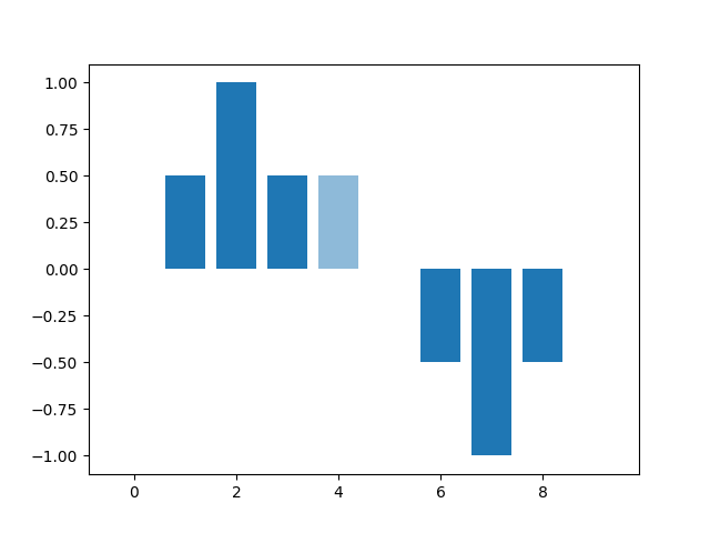 Figure 1
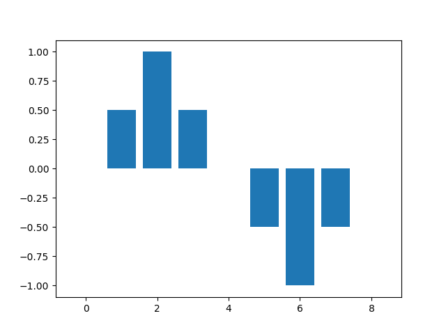 Figure 2
Peer Reviews
No public reviews on file for this paper yet. If you reviewed it on a platform where reviews are public (OpenReview, ICLR, NeurIPS, ICML), you can paste yours below so the community can read it here.
Code & Models
Videos
No videos yet. Explain this paper in a talk, walkthrough, or lecture? Add one.
Time-warping invariants of multidimensional time series
Joscha Diehl
Universität Greifswald, Institut für Mathematik und Informatik, Walther-Rathenau-Str. 47, 17489 Greifswald, Germany.
,
Kurusch Ebrahimi-Fard
Department of Mathematical Sciences, NTNU, 7491 Trondheim, Norway.
and
Nikolas Tapia
Weierstraß-Institut Berlin, Mohrenstr. 39, 10117 Berlin, Germany
Technische Universität Berlin, Str. des 17. Juni 136, 10623 Berlin, Germany.
Abstract.
In data science, one is often confronted with a time series representing measurements of some quantity of interest. Usually, in a first step, features of the time series need to be extracted. These are numerical quantities that aim to succinctly describe the data and to dampen the influence of noise.
In some applications, these features are also required to satisfy some invariance properties. In this paper, we concentrate on time-warping invariants. We show that these correspond to a certain family of iterated sums of the increments of the time series, known as quasisymmetric functions in the mathematics literature. We present these invariant features in an algebraic framework, and we develop some of their basic properties.
Key words and phrases:
Time series analysis, time warping, standing-still invariance, signature, quasisymmetric functions, quasi-shuffle product, Hoffman’s exponential, area-operation, Hopf algebra
2020 Mathematics Subject Classification:
60L10, 16T05, 62M10, 68T10
1. Motivation
Given a discrete time series
[TABLE]
where is some arbitrary time horizon, our foremost, and original, motivation stems from the desire to extract features from that are invariant to time warping.
The precise definition of the latter will be given in Section 4, but Figure 1 illustrates what we mean by time warping: the time series is allowed to “stand still” or to “stutter” (this term is used in [47]), which means that has repetitions of values at consecutive time steps (here at time ).
Remark 1.1**.**
In this section we consider the notationally simpler case , that is, when .
Our interest is prompted, on the one hand by the extensive literature on the dynamic time warping (DTW) distance [5], a distance on discrete time series that is invariant to time warping. In [47] it is stated that
“the time warping distance …does not lead to any natural features”.
Our work aims to provide those missing “natural” features.
On the other hand the following example illustrates where such invariant features will become useful.
Example 1.2**.**
Assume that there is a deterministic time series which models some “prototype” evolution of a quantity, say the prototype heartbeat in a patient’s ECG. This prototype is unknown, but one records a lot of samples of it run at different speeds and contaminated by noise (compare [6]). A model for these observations is then
[TABLE]
Here is the number of observations, is the time horizon we allow the prototype to be “spread out” over, are unknown non-decreasing, surjective time changes and are independent and identically distributed (iid) random walks. The goal is to recover (up to time warping).
The currently used method [6, 31, 33], consists in first trying to align the different samples, i.e., to estimate the time-changes , and to average afterwards. This seems to work well in regimes where the noise is small (large signal-to-noise ratio), but will break down if this is not the case.
Guided by invariant methods in cryo-EM [4] we then propose the following procedure.
- (1)
Calculate features of that do not see time warpings. 2. (2)
Average those features over the independent samples, giving the law of large numbers a chance to cancel out the noise and getting an approximation of the features of . 3. (3)
Invert the averaged features to arrive at a candidate for .
Our approach to Step (1) is new and will be presented in this paper. Step (2) and Step (3) will be addressed in future work.
A moment’s thought reveals that iterated-sums of the increments of are invariant in the desired sense. For example, the simple sum or the more complex expressions
[TABLE]
are features of the time series that do not change when warping time, i.e., when repetitions of points, occur in .
Remark 1.3**.**
To accommodate repetition of points, here we have conveniently written the sum over an unspecified set of time-points. We can think of the sum taken over , with being extended constantly as after time .
However, two questions immediately emerge
- (A)
The three expressions in (1) are already linearly dependent (adding the first and second sum gives the third). How to store only linearly independent expressions? 2. (B)
Do iterated-sums of increments give all (polynomial) time warping invariants?
Regarding the first item, it turns out that the above iterated-sums expressions are reminiscent of quasisymmetric functions [39]. Consider the space of formal power series in ordered commuting variables . By definition, a power series (of finite degree) is a quasisymmetric function if for all , all , all and all , the coefficient of the monomial in is equal to the one of . First examples are
[TABLE]
and we see that the invariants given above follow from the evaluation of these quasisymmetric functions at , and for .
Different linear basis for quasisymmetric functions are known. The one of monomial quasisymmetric functions of [39] is indexed by compositions of integers. Anticipating the multidimensional case, we write a composition as , and obtain the correspondence
[TABLE]
Quasisymmetric functions are a refinement of symmetric functions and form a commutative unital algebra. The product is just the polynomial product in the power series representation. It amounts to a so-called quasi-shuffle product (see Section 2) in the representation as compositions. For example, the abstract quasi-shuffle product
[TABLE]
corresponds to the concrete product of power series
[TABLE]
The latter equality follows by case distinction for sums over the three indexing variables, which amounts to a summation-by-parts formula. The last two terms in the above product reflect the fact that multiplying sums requires the inclusion of sums over diagonal terms.
It is natural to store the iterated-sums invariants of the discrete time series as a linear map on the quasi-shuffle algebra of compositions, by defining the pairing
[TABLE]
Here for , and as above we extend constantly, so that for . From the correspondence between the product of power series and the quasi-shuffle product of compositions mentioned above we deduce that
[TABLE]
Hence, , which we call iterated-sums signature, is an algebra morphism (from the quasi-shuffle algebra to the underlying base field ). Since compositions form a linear basis, this answers Question (A) above – in the case . We will come back to Question (B) in Section 4.
The commutative algebra of quasisymmetric functions is the free quasi-shuffle algebra over one generator and it is - as we just saw - the correct framework to store iterated-sums for a one-dimensional time-series. The appropriate generalisation of this algebra to arbitrary dimension , that is, the free quasi-shuffle algebra over generators, was carried out by Hoffman [27].
The aforementioned amounts to saying that iterated-sums signature is an element of the dual space of the quasi-shuffle algebra over generators. It can therefore be represented as an infinite word series with iterated-sums of the time series as coefficients. Its compatibility with the quasi-shuffle product together with the fact that the latter can be seen as a deformation of the classical shuffle product [18] suggests to consider as a discrete analog of Chen’s iterated-integrals signature over continuous curves [10, 44]. The latter plays an important role in the theory of controlled ordinary differential equations (ODEs), stochastic analysis and Lyons’ theory of rough paths [19, 37]. Such a large spectrum of applications reflects the important property of iterated-integrals to provide - in some sense - a complete representation of a curve, so that arbitrary functionals on curves should be well approximated by functions on its signature. There is a caveat though. Iterated integrals are tailor made to approximate functionals that stem from controlled ODEs. But as is quickly realised, this does not mean that the iterated-integrals signature is an optimal representation for other input-output systems. For example, since a controlled ODE - and hence also the signature - cannot see tree-like excursions, the iterated-integrals signature of a one-dimensional path reveals nothing about the path, except for its increment.There are several procedures to circumvent this shortcoming, and to obtain information even about tree-like parts of a curve using signature. These procedures usually consists of lifting the path to a higher-dimensional curve and calculating the signature of it. The aforementioned limitations of the iterated-integrals signature with respect to tree-like paths prompts us to propose instead the use of “discrete time signature” , which, instead of storing iterated-integrals, gathers iterated-sums.
Remark 1.4**.**
For the precise definition of “tree-like” see [24]; but one can think of a curve that completely “tracks back”. In particular in dimension , every curve that has coinciding start- and endpoint is tree-like.
The paper is organised as follows. Section 2 recalls the notion of quasi-shuffle Hopf algebra and quasisymmetric functions. In Section 3 we introduce the iterated-sums signature and show its character property with respect to the quasi-shuffle Hopf algebra. Moreover, we show that Chen’s property is satisfied, but that Chow’s Theorem does not hold. Hence, while mirroring the setup of Chen’s iterated-integrals signature to some extent, interesting differences emerge. It turns out that our description of the iterated-sums signature is nicely related to the work [42] on “multidimensional” generalisation of quasisymmetric functions, and we dwell on this briefly in Remark 3.5. In Section 4 we show the iterated-sums signature contains (almost) all time warping invariants. In Section 5 we use a specific Hopf algebra isomorphism, known as Hoffman’s exponential, to relate the iterated-sums signature to Chen’s iterated-integrals signature (of an infinite-dimensional path). This includes in particular relating the continuous and discrete area operations.
In the following all algebraic structures are defined over a base field of characteristic zero. The reader is invited to think of the field as the reals, , or the complex numbers, , throughout.
We denote and . All (co)algebras are (co)unital and (co)associative unless otherwise stated. For details on Hopf algebras the reader is referred to [9, 26, 36, 40, 46].
2. Quasi-shuffle Hopf algebra
The notion of quasi-shuffle product appeared first in a 1972 article by Cartier [8]. Its Hopf algebraic relevance was explored in the 1979 paper [41]. Two decades later, Hoffman [27] provided a comprehensive account of the quasi-shuffle product in a Hopf algebraic framework. Meanwhile, quasi-shuffle products appeared under different names, i.e., modified shuffle product [20, 34], sticky-shuffle [29, 30], overlapping shuffle [25], stuffle and harmonic product [48].
We recall the inductive definition of the quasi-shuffle product following Hoffman [27]. See also [7, 16]. Our starting point is the alphabet , which we augment to a free commutative semigroup, , by defining a commutative product denoted by square brackets, . For example, the product between the letters is written . Any iteration of the product in can be simplyfied to an expression containing a single pair of brackets, that is, . For instance, in . Elements in the tensor algebra over (the vector space spanned by) are denoted by words, i.e., we denote the tensor product by concatenation, or juxtaposition of basis elements. The neutral element for this product is the empty word, denoted by . The augmentation ideal is defined by such that .
The commutative quasi-shuffle product , , is introduced by inductively defining , for all , and
[TABLE]
for and . For example, and
[TABLE]
The tensor algebra is naturally graded by the length of words, for . However, in light of the new product (2), which is not homogenous with respect to the number of letters, we introduce the weight grading on , denoted , by declaring that , for all and for all . Finally, for a word we define its weight to be .
Let denote the deconcatenation coproduct defined on a nonempty word by
[TABLE]
and . It turns into a connected graded coalgebra, for both the length and weight grading. For any word the reduced coproduct is defined by . “Sweedler’s notation” will be employed for both coproducts: and . The canonical counit map is defined to be and zero on . In [27] Hoffman showed the following
Theorem 2.1** (Quasi-shuffle Hopf algebra).**
1. is a graded, connected, commutative, non-cocommutative Hopf algebra.
2. The antipode is given by
[TABLE]
Here is the set of all compositions of the integer , i.e., tuples of positive integers such that . Given and a word of length , we define a new word by
[TABLE]
Here (as well as later) we are using the suitable convention that for all .
Remark 2.2** (Shuffle Hopf algebra).**
If the semigroup is trivial, i.e., if for any letters , then the quasi-shuffle product (2) reduces to Chen’s commutative shuffle product on :
[TABLE]
for and . Observe that in this case for any word and is the classical shuffle Hopf algebra over the alphabet . From (5) it follows that the antipode on is given by . See [46] for a comprehensive account on .
Remark 2.3** (A remark on dimensions.).**
There is a simple way of computing the Hilbert series
[TABLE]
of , where is the homogeneous (for the weight grading) component of degree of the quasi-shuffle algebra. It is not hard to see that all such words are of the form for some composition and letters , in the notation of Theorem 2.1. In total, in each block of size we are allowed to put a symmetric monomial of length of which there are exactly – this is the dimension of the degree- part of the symmetric algebra . Therefore
[TABLE]
A simple computation shows that in fact
[TABLE]
where the Pochhammer symbol (or rising factorial) appears on the righthand side. It is well known that their exponential generating function equals the hypergeometric function
[TABLE]
Therefore
[TABLE]
The coeffficients of these Hilbert series can be found in column of the OEIS sequence A261780.
Define the scalar product for any words by if and zero else. It permits to identify the graded dual of as word series, i.e., , which is a non-commutative (topological) Hopf algebra with concatenation as convolution product, denoted by , , and de-quasi-shuffling as coproduct [27]. In more concrete terms, this means that given two such series their convolution product may be written as
[TABLE]
Of particular interest are characters, i.e., algebra morphisms . They satisfy and , for . The first property requires that the coefficient and the second is equivalent to being group-like in , which means that for
[TABLE]
where the de-quasi-shuffling coproduct is defined on words by
[TABLE]
The set of characters, denoted by , forms a group with the inverse . The corresponding Lie algebra, , consists of so-called infinitesimal characters, which map the empty word and any non-trivial product in to zero. One can define the exponential map as a power series with respect to the convolution product which maps bijectively to , i.e., . Because is a graded connected Hopf algebra, this expression becomes a finite sum when evaluated on homogeneous elements of , so we do not have to deal with convergence issues. Its inverse is the logarithm, . Again, the sum applied to any word terminates after terms, as .
Notation 2.4**.**
We introduce a particular notation for words in , which will be useful in the sequel. The convention to identify , for , permits to write any word in as a concatenation of brackets, i.e., , for .
We come back to the setting of the introductory section with only a single letter, . Then, in each degree , has a single word of length one, , and any basis element (or word) is of the form for some integers . It is easy to see that then the tuple is a composition of the integer of length . In [27] Hoffman describes a unital algebra isomorphism between the quasi-shuffle algebra , for , and the algebra of quasisymmetric functions in the ordered set of commuting variables [21], defined by taking a word in to an iterated sum
[TABLE]
Here . Then, the correspondence of the introduction is explicitly given by
[TABLE]
where the second equality is an example of summation-by-parts for products of iterated sums.
The of (6) are the monomial quasisymmetric functions, which form a basis for . The Hopf algebra is a generalisation of the classical Hopf algebra of symmetric functions. It was defined and studied by Gessel [21], based on earlier work by Stanley, and plays a rather distinguished role in modern algebraic combinatorics, with ramifications into several other fields of mathematics. Its graded dual is known as the connected graded cocommutative Hopf algebra of noncommutative symmetric functions. The iterated-sums signature corresponding to a one dimensional discrete time series, alluded to in the first section, is an element in . Further below, in Section 3, we consider the multidimensional generalisation of quasisymmetric functions (of level in the terminology of [42]) and its corresponding iterated-sums signature. We close this section by mentioning that Malvenuto’s and Reutenauer’s Hopf algebra of permutations [39] plays an important part in the understanding of the relation between the objects , and . The interested reader is referred to [2, 1] and to [36] for a readable introduction, including a brief historical overview.
2.1. Half-shuffles
Aiming at understanding the discrete analog of the operation (to be introduced further below), we take a more refined approach at the quasi-shuffle product by observing that may be split into three products, i.e., left and right half-shuffles and a third product
[TABLE]
so that . For instance (c.f. Example 3)
[TABLE]
Noticing the particular relation which is equivalent to being commutative, it is not hard to show that the quasi-shuffle algebra becomes a commutative tridendriform algebra, , as defined by Loday and Ronco [35].
Remark 2.5**.**
A similar splitting holds for the shuffle algebra in Remark 2.2. We can write the shuffle product on as a sum of the two half-shuffles
[TABLE]
so that . Again, we check quickly that the commutativity of the shuffle product is equivalent to . In fact, the triple is also known as a commutative dendriform or Zinbiel algebra.
2.2. Hoffman’s exponential
Shuffle and quasi-shuffle Hopf algebras are more tightly related than Remark 2.2 may adumbrate. Indeed, Hoffman proved in [27] that and are isomorphic as Hopf algebras. We briefly recall this result. Let be equipped with the commutative shuffle product inductively defined by , for and . The empty word, , is the unit for this product. Recall the notation introduced in Theorem 2.1.
Theorem 2.6** (Hoffman’s isomorphism).**
[27]** There exists a Hopf algebra isomorphism , given explicitly by the so-called Hoffman exponential
[TABLE]
Its inverse also admits an explicit expression, namely the Hoffman logarithm
[TABLE]
Some examples: and for the words and we find
[TABLE]
In the second example, the terms correspond to the compositions , , and of the integer , in that order. Recall that the particular Notation 2.4 for words , for , is in place. Also, note that the number of letters in each of the terms corresponds to the length of the composition. The reader is referred to [27, 28] for more details. See also [16] for an application in stochastic analysis.
In Section 5 we will show that is nicely compatible with comparing the iterated-sums signature on one side with the iterated-integrals signature on the other. The following two lemmas are going to be used in Section 5.1, where we address the area operation in the context of the iterated-sums signature.
Lemma 2.7**.**
The image of any nonempty word under Hoffman’s isomorphism can be split into two parts as follows:
[TABLE]
where the remainder term
[TABLE]
The verification of the lemma is left to the reader. This splitting of Hoffman’s isomorphism implies the following important result.
Lemma 2.8**.**
Let and . Then
[TABLE]
Proof 2.9**.**
From Lemma 2.7 and linearity of , we deduce that
[TABLE]
Since the semigroup is commutative, for any composition with we have that
[TABLE]
Therefore, the equality holds, which implies the identity (12).
3. Iterated-sums signatures
We consider a discrete time series as an element of
[TABLE]
the space of infinite time series that are eventually constant, by extending it constantly. In this section we will see that the appropriate algebraic setting for iterated-sums, combined into the map , is that of a character on the quasi-shuffle Hopf algebra over the semigroup corresponding to the alphabet , introduced in Section 2.
The following notation for elements in the time series is put in place:
[TABLE]
Next we define the corresponding time series
[TABLE]
with increments , for , as entries. The new notation is extended to include all brackets in by defining
[TABLE]
Definition 3.1**.**
The iterated-sums signature of the time series is the two-parameter family of linear maps from to such that , and defined recursively by , and for
[TABLE]
Hence, the iterated-sums signature is a word series in
[TABLE]
with iterated sums over increments of as coefficients, defined as
[TABLE]
For example
[TABLE]
We extend this definition to all by setting whenever .
Remark 3.2**.**
An easy consequence of this definition is that the coefficient vanishes whenever .
The proof of the following lemma is straightforward.
Lemma 3.3**.**
Let and be two time series, and denote by . Then the increment of the product is given by a generalised Leibniz rule
[TABLE]
More importantly, we have the following:
Theorem 3.4**.**
- (1)
(Quasi-shuffle identity)* For each , the map is a quasi-shuffle Hopf algebra character.* 2. (2)
(Chen’s property)* For any three we have*
[TABLE]
Remark 3.5**.**
1. Observe that point (i) in Theorem 3.4 amounts to a generalisation of the algebra isomorphism defined in (6) to the multidimensional case, i.e., for an alphabet . Indeed, defining the map on
[TABLE]
where and for we have set
[TABLE]
we obtain a quasi-shuffle algebra isomorphism into the algebra of quasi-symmetric functions of level , as introduced by Novelli and Thibon in [42]. For the sake of briefness we only remark that
[TABLE]
2. Specialising to , Theorem 3.4 matches the corresponding result for the iterated-integrals signature of a curve of bounded variation in , where is a (possibly countable) alphabet. The iterated-integrals signature is also called Chen’s signature, rough path signature, continuous-time signature or just signature in the literature.
Here, the underlying Hopf algebra is . Indeed (see for example [23]),
- (1)
(Shuffle identity)* For fixed , is a character on , that is for all *
[TABLE] 2. (2)
(Chen’s property)* For *
[TABLE]
Before proving Theorem 3.4 we need the following abstract result, which is a particular case of the setting presented in [42, Section 5.1].
Lemma 3.6**.**
Let denote the level monomial quasisymmetric functions defined in (15). Then, the “generating series”
[TABLE]
admits the factorisation
[TABLE]
Let us look at the first few terms in (16):
[TABLE]
Instead of elaborating on this lemma, we refer to reference [42] for details about multivariable generating series. Note, however, that after evaluating in , we obtain and the factorisation (16) takes place in the convolution algebra . We further remark that the expansion of the geometric series on the righthand side of the first equality in (16) takes place in , which explains the summation over in the second equality.
Remark 3.7**.**
Equality (16) bears resemblance to [32, Definition 4.1] (c.f. also [38, Theorem 32]. We would like to thank Harald Oberhauser (Oxford) for pointing us to these references). At first sight though, only coefficients for words in letters of weight one are considered in the aforementioned reference (e.g. in our notation …). Preprocessing the underlying time series through a nonlinear function (i.e. a kernel in the terminology of [32]), one can introduce additional polynomial expressions. But, note that in their setting then nonetheless sums of increments of polynomials appear, whereas in the iterated-sums signature (i.e. in (16) evaluated at ) polynomials of increments show up.
The differences between the two approaches may be summarized by saying that increments of polynomials differ from polynomials of increments. Saying this, it is an interesting question how these two approaches could be combined fruitfully. In particular, we hope to investigate the application of kernelization techniques to the iterated-sums signature.
Finally, we would like to mention that the work of Hoffman–Ihara (see Section 5 and [28], as well as [18]) permits to define for any positive integer a linear automorphism of which gives rise to a family of “feature maps” interpolating between the iterated-sums signature and the iterated-integrals signature. This relates to a modification of (16) in the spirit of [32, Appendix B]. These new feature maps define characters over Hopf algebras equipped with new quasi-shuffle type products. The corresponding family of linear automorphisms define algebra maps between these quasi-shuffle type products and the quasi-shuffle product (2). We postpone the details of this construction to a follow-up paper, and would like to thank the anonymous referee for hinting at this direction.
Proof 3.8** (Proof of Theorem 3.4).**
1. We need to show that for words
[TABLE]
We use the recursive definition of the quasi-shuffle product (2) and induction on , the base case (i.e., or ) being trivial. If and , define the auxiliary time series
[TABLE]
for , and zero else. Observe that the increments
[TABLE]
By the induction hypothesis we then get
[TABLE]
and similarly
[TABLE]
Also, by a similar argument we also have
[TABLE]
Finally, we summate these relations by using Lemma 3.3 to get
[TABLE]
2. The proof of Chen’s property can be pursued using a pedestrian approach. However, it also follows from Lemma 3.6. Indeed, we may split the product in the factorisation (16) as
[TABLE]
The desired identity follows upon evaluation at as in the previous remark.
We note that the iterated-sums signature, , introduced in this work is similar to the discrete Chen(–Fliess) series defined and studied in [22] in the context of nonlinear control theory.
This section is closed with an intriguing observation. Up to this point it may seem that iterated-sums signatures, , and Chen’s signatures, (see Remark 3.5), behave in the same way, but as the next example shows this is not at all the case. Recall that , the space of linear maps on , together with the convolution product is a non-commutative algebra with unit , where is the unit map, . Define
[TABLE]
where is the projection onto the augmentation ideal . It is the adjoint of the classical Eulerian Lie idempotent [46], that is, the concatenation logarithm of the identity map, . Observe that the sum (17) terminates when evaluated in homogeneous elements since , thus it is well defined for arbitrary elements of . Then, for any character and word we have that
[TABLE]
where . Indeed, by definition
[TABLE]
In the third equality we used that is a character. In the second equality the reduced coproduct is applied
[TABLE]
Now, if is an arbitrary time series, for its iterated-sums signature this means that
[TABLE]
Therefore, the image of the logarithm of iterated-sums signatures only reaches a certain subset of the Lie algebra of infinitesimal characters on . This is in contrast to Chen’s iterated-integrals signature, for which Chow’s Theorem [19, Theorem 7.28] holds, showing that any character over the shuffle Hopf algebra may be realised as the Chen signature of a piecewise linear path. The implications of this observation will be studied in a forthcoming paper.
Still, the following positive statement on the linear span of iterated-sums signatures holds.
Lemma 3.9**.**
For every , .
Remark 3.10**.**
The corresponding result for iterated-integrals signatures was shown in [13, Lemma 3.4], which is sometimes useful for proving statements about the underlying algebra that are easily verified when tested against signatures.
Proof 3.11**.**
Fix and let , ordered in some way, be the quasisymmetric monomial functions with degree smaller or equal to .
By [42, Section 5.1] they are independent as elements of the space of formal power series.
This implies that, for some large enough, evaluating at , the expressions are independent as elements of . Denote
[TABLE]
copies in new variables of , that is . Then, the independence of the implies independence, in , of the rows of
[TABLE]
A fortiori, also the columns must be independent in . Hence, the columns must be independent for some realisation of the . This finally implies that we can find such that the columns of
[TABLE]
are independent. Here, as before, we extend the constantly to an element of .
4. Invariants
In the previous section, we defined the iterated-sums signature, following the introduction. We now return to our original motivation, and first put the concept of “time warping” in a precise mathematical framework. For each index we define an operator acting on sequences by repeating once the value at time . More precisely, given a time series, , we define as the time series given by
[TABLE]
Observe that with this definition we have , and the rest of the values are unchanged save for a time shift after time .
Definition 4.1**.**
We call a functional invariant to time warping if for all .
From applications to data analysis, such as, e.g., moment corrections, we are mostly interested in polynomial invariants, i.e., invariant functionals that can be expressed by considering only polynomial expressions in a time series.
Definition 4.2**.**
We call polynomial, if for all , is a polynomial in the , and the polynomial degree is uniformly bounded in .
From the factorisation (16) in Lemma 3.6 it follows that for any word the coefficient is a polynomial invariant in this sense. It turns out these are all the polynomial invariants, if we additionally demand invariance with respect to space translation of the entire series.
Lemma 4.3**.**
Let be polynomial, invariant to both time warping and space translations. Then: is realised as a quasisymmetric function.
Proof 4.4**.**
We do the one-dimensional case, , to avoid notational clutter. By translation invariance, for any ,
[TABLE]
Now, by assumption, this is a polynomial in hence it is a (different) polynomial in . Therefore, can be realised as a formal power series of bounded degree: there is of bounded degree such that for we have that .
It remains to show that is quasisymmetric. Let , and . We show that the coefficient of the monomial in is equal to the one of .
Indeed: by using repeatedly the invariance to time warping, we get that for all ,
[TABLE]
Hence, both sides coincide as polynomials. So that the coefficient of and must coincide. This finishes the proof.
5. Hoffman’s isomorphism and signatures
In this section we relate the iterated-sums signature of a time series with the usual iterated-integrals signature of the piecewise linear interpolation of an associated infinite dimensional time series.
Starting again with the extended alphabet , we build the tensor algebra and define the shuffle product inductively by
[TABLE]
Recall Hoffman’s isomorphism [27] defined in Theorem 2.6, which shows that and are isomorphic as Hopf algebras. Next we compute explicitly the image by the iterated-integrals signature of a linear path.
The following lemma is an immediate extension of [19, Example 7.21] to a countable index set.
Lemma 5.1**.**
Consider a countable set and let for some and all . Then for
[TABLE]
At the level of the tensor algebra this simply means that . An analogue of this result holds for discrete signatures, which follows from Lemma 3.6, i.e., Chen’s property.
Lemma 5.2**.**
Let be a time series having a single non-zero increment . Then
[TABLE]
Now we look for a relation between the iterated-integrals signature and the iterated-sums signature. For this, let be a time series and consider the (infinite dimensional!) path where, for , the component path is the linear interpolation of the time series
[TABLE]
Theorem 5.3**.**
We have .
Remark 5.4**.**
We note that the iterated-integrals signature of the -dimensional path consisting in the piecewise linear interpolation of is not enough to obtain . Instead, the theorem shows that the iterated-integrals signature of the piecewise linear interpolation of the infinite dimensional time series (18) is sufficient.
Proof 5.5**.**
Without loss of generality let the interpolation of (18) happen at the time points . Then, by Chen’s property,
[TABLE]
We first investigate what happens for a single time step. Let a word be given, and write , . According to Lemma 5.1,
[TABLE]
where . In other words, is the number of times the letter is repeated in .
Now the only term in containing a single letter is , i.e., the full “contraction”. Then, by Lemma 5.2,
[TABLE]
Therefore, we have shown the claim for a single time step.
Now, since is a Hopf algebra map, the statement of the theorem is equivalent to showing that , where is the adjoint of Hoffman’s isomorphism. Since is an algebra morphism, we calculate
[TABLE]
So the result is valid for the full signature.
Finally, we show a consistency result.
Proposition 5.6**.**
Let be a continuous path of finite variation, meaning that
[TABLE]
where the supremum is taken over all partitions of .
Given such a partition , define by . Then
[TABLE]
Proof 5.7**.**
We use induction on the length . If and , then
[TABLE]
which is independent of . If, on the other hand, then with . Therefore
[TABLE]
which vanishes in the limit since is uniformly continuous on .
Now suppose for some and . We have 3 cases
- (1)
: in this case, no matter what is, we have
[TABLE]
as , by the induction hypothesis. 2. (2)
* and : the same argument as before gives that the corresponding entry in vanishes in the limit.* 3. (3)
* and : again by definition we have*
[TABLE]
which converges to the Young (or Riemann–Stieltjes) integral
[TABLE]
Therefore, we have that
[TABLE]
if , and vanishes otherwise.
5.1. The area operation
It is well known that for the iterated-integrals signature certain linear combinations of the entries have a precise geometric interpretation. Indeed, for any
[TABLE]
represents (two times) the signed area (or Lévy area) between the curves and for , and the cord between the points and .
We abstract this operation to the shuffle algebra by using the notion of half-shuffles introduced in Section 2.1. In fact, one verifies that at this level the area operation may be represented in terms of half-shuffle operations as
[TABLE]
so that in particular .
We extend this by defining area operations on and .
Definition 5.8**.**
The area map is defined by
[TABLE]
Next, the discrete analogue is given in terms of the first half-shuffle product in (7).
Definition 5.9** (Discrete area).**
The discrete area map is defined by
[TABLE]
We compare the two areas by considering the words and . Then
[TABLE]
as follows from Example 8.
Both and can be iterated. We now make this precise: define , the vector space spanned by the set . Then, inductively define vector spaces
[TABLE]
We finally set
[TABLE]
Neither the nor the discrete operations are associative. One can show, however, that satisfies a fourth-order relation, known as tortkara, introduced by Dzhumadil’daev in the 2007 paper [14]. In [15] the image of iterated applications of the area map is characterised. (Compare also [45, Theorem 28]).
Theorem 5.10** ([15, Theorem 2.1]).**
The space is spanned by the set
[TABLE]
From Lemma 2.7 and Lemma 2.8 we deduce the following morphism property of Hoffman’s isomorphism with respect to and .
Theorem 5.11**.**
* is a tortkara morphism, i.e., for *
[TABLE]
Remark 5.12**.**
1. Note that is not a (quasi-)half-shuffle morphism. Only the anti-symmetrisation to respectively is nicely compatible with it.
2. The set (the set of “areas-of-areas”) is known to generate as a shuffle-algebra, see [12]. Applied to iterated-integral signatures this means that all their information is already contained in areas-of-areas. The area operation has an immediate geometric interpretation, whereas the operation of integration .111The authors would be hard-pressed to explain the latter to a non-mathematician, whereas the former can be explained by a simple drawing. Moreover, the area operation is related to antisymmetrised lead-lag correlation in time series analysis, see [13, Section 3.2]. We refer to [12, Section 6] for more applications.
Proof 5.13**.**
By Dzumadil’daev’s theorem (Theorem 5.10) it suffices to prove the claim for the case when and . We first observe that in this case the operation can be written more explicitly:
[TABLE]
Each of these terms can be further expanded into three terms. For example, the first one equals
[TABLE]
In total there are 12 terms, the remaining 9 terms are
[TABLE]
For each of these terms we can find exactly one other term such that their sum is of the form , for , and thus by Lemma 2.8 the image of this sum has the form . To summarise, the image is a linear combination of 6 terms, each of them having the form . Now, if we pick any there are exactly three terms containing as the last letter. For example, for these terms are
[TABLE]
where the last identity is easy to check using that . Applying a similar argument to all letters we see that
[TABLE]
6. Conclusion
In this work we have
- •
introduced a new set of features for multidimensional time series consisting in iterated sums (Section 3);
- •
shown that these features are invariant to time warping and that these in fact are all the (polynomial) invariants in this sense (Section 4);
- •
described a Hopf algebraic framework to compute these features (Section 2);
- •
shown how this setting mirrors the one of iterated-integrals in some aspects and differs in others (Section 2).
There are several possible generalisations of our work.
- •
Let be such that . Then iterated-sums of the form
[TABLE]
are also invariant to time warping (and analogously for higher order iterated-sums). These are, in general, not polynomial in the time series anymore, but might still be relevant for certain applications. For smooth this should be related to the expansion of nonlinear functionals on stochastic word series [11], but the non-smooth case (for example , ) is particularly interesting.
- •
Multi-parameter data. An object of interest are for example “images” and the time warping invariance becomes an invariance to stretching of the image.
We are also interested in exploring the possible applications of these invariants in data science.
- •
Retrieval of similar time series, invariant to time warping: see [47] (and references therein), where it is stated that “the time warping distance …does not lead to any natural features”. The invariants presented in our work should provide those missing features, but a mathematical rigorous proof of this statement is left for future work.
- •
Statistical inference in problems involving unknown time warping, as in Example 1.2.
- •
Time series clustering: the features of this work can be used to cluster time series according to their “shape”, i.e., independent of time warping. Sometimes a “prototype” for each cluster is looked after, see for example [43]. In this case - as in the previous point - reconstruction of a time series from an (averaged) iterated-sums signature would be necessary. A detailed study of this ostensibly hard problem is left for future research.
We close with some open questions. At the end of Section 3 we showed that an equivalent of Chow’s theorem does not hold for the iterated-sums signature .
- •
Can we understand as a semi-algebraic set? (Compare [3] for the investigation of the image of iterated-integrals signatures as algebraic sets.)
- •
For denote by the time series run backwards. Then (as might surprise readers familiar with Chen’s signature) . What are the implications?
- •
The lead-lag procedure of [17] lifts a discrete time series of dimension to a piecewise smooth curve of dimension . Since the resulting iterated-integrals signature is invariant to time warping as well as space translations, and is polynomial in the original time series, by Lemma 4.3 it must be contained in the iterated-integrals signature . Conversely, is the signature of the resulting curve enough to recover the iterated-sum signature? This would give a finite dimensional smooth curve whose iterated-integrals signature contains the invariants presented in this paper (compare Theorem 5.3 for an infinite dimensional smooth curve doing the job).
Acknowledgments The authors would like to thank the referee for valuable remarks and comments, in particular with respect to reference [32]. N.T. kindly acknowledges support from the European Research Consortium for Informatics and Mathematics through post-doctral fellowship ERCIM 2018-10 and from the Excelence Cluster MATH+ EF1.
The reference list from the paper itself. Each links out to its DOI / PubMed record.
- 1[1] M. Aguiar, N. Bergeron, and F. Sottile, “Combinatorial Hopf algebras and generalized Dehn–Sommerville relations,” Compos. Math. 142 no. 01, (2006) 1–30 . · doi ↗
- 2[2] M. Aguiar and F. Sottile, “Structure of the Malvenuto–Reutenauer Hopf algebra of permutations,” Adv. Math. 191 no. 2, (Mar, 2005) 225–275 . · doi ↗
- 3[3] C. Amendola, P. Friz, and B. Sturmfels, “Varieties of signature tensors,” in Forum of Mathematics, Sigma , vol. 7, Cambridge University Press. Cambridge University Press (CUP), 2019. · doi ↗
- 4[4] A. S. Bandeira, B. Blum-Smith, J. Kileel, A. Perry, J. Weed, and A. S. Wein, “Estimation under group actions: recovering orbits from invariants,” ar Xiv:1712.10163 [math.ST] .
- 5[5] D. J. Berndt and J. Clifford, “Using Dynamic Time Warping to Find Patterns in Time Series,” in Proceedings of the 3rd International Conference on Knowledge Discovery and Data Mining , AAAIWS’94, pp. 359–370. AAAI Press, 1994.
- 6[6] J. Bigot, “Fréchet means of curves for signal averaging and application to ECG data analysis,” Ann. Appl. Stat. 7 no. 4, (2013) 2384–2401 . · doi ↗
- 7[7] Y. Bruned, C. Curry, and K. Ebrahimi-Fard, “Quasi-shuffle algebras and renormalisation of rough differential equations,” ar Xiv:1801.02964 [math.CA] .
- 8[8] P. Cartier, “On the structure of free Baxter algebras,” Adv. Math. 9 (1972) 253–265 . · doi ↗
