TL;DR
This paper determines the rank of sparse random matrices over any field with fixed row and column sparsity, providing a formula for low-density parity check codes and confirming Lelarge's conjecture.
Contribution
It introduces a new method involving random perturbation to analyze the rank of sparse matrices, applicable across various fields.
Findings
Derived a formula for the rank of sparse random matrices
Confirmed Lelarge's conjecture on LDPC code rates
Developed a novel perturbation technique for matrix analysis
Abstract
We determine the rank of a random matrix over an arbitrary field with prescribed numbers of non-zero entries in each row and column. As an application we obtain a formula for the rate of low-density parity check codes. This formula vindicates a conjecture of Lelarge (2013). The proofs are based on coupling arguments and a novel random perturbation, applicable to any matrix, that diminishes the number of short linear relations.
Click any figure to enlarge with its caption.
 Figure 1
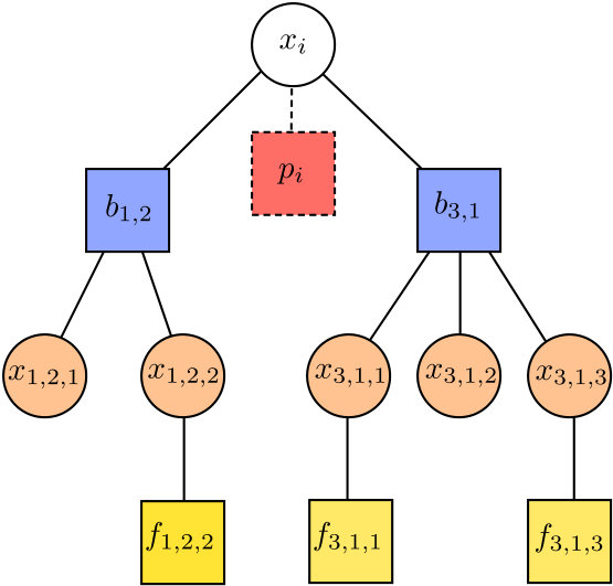 Figure 2
 Figure 3
 Figure 4
 Figure 5
Peer Reviews
No public reviews on file for this paper yet. If you reviewed it on a platform where reviews are public (OpenReview, ICLR, NeurIPS, ICML), you can paste yours below so the community can read it here.
Videos
The Rank of Sparse Random Matrices· youtube
The rank of sparse random matrices
Amin Coja-Oghlan, Alperen A. Ergür, Pu Gao, Samuel Hetterich, Maurice Rolvien
Amin Coja-Oghlan, [email protected], TU Dortmund, Faculty of Computer Science, 12 Otto Hahn St, Dortmund 44227, Germany.
Alperen A. Ergür, [email protected], The University of Texas at San Antonio, TX, USA.
Pu Gao, [email protected], Department of Combinatorics and Optimization University of Waterloo, Canada.
Samuel Hetterich, [email protected], Goethe University, Mathematics Institute, 10 Robert Mayer St, Frankfurt 60325, Germany.
Maurice Rolvien, [email protected], TU Dortmund, Faculty of Computer Science, 12 Otto Hahn St, Dortmund 44227, Germany.
Abstract.
We determine the asymptotic normalized rank of a random matrix over an arbitrary field with prescribed numbers of non-zero entries in each row and column. As an application we obtain a formula for the rate of low-density parity check codes. This formula vindicates a conjecture of Lelarge (2013). The proofs are based on coupling arguments and a novel random perturbation, applicable to any matrix, that diminishes the number of short linear relations. MSC: 05C80, 60B20, 94B05
Coja-Oghlan supported by DFG CO 646/3 and 646/4. Ergür’s research was partially supported by Einstein Foundation, Berlin and NSF CCF 2110075. Gao’s research is supported by ARC DE170100716 and ARC DP160100835. This submission combines the preprints arXiv:1810.07390 and arXiv:1906.05757. An extended abstract of this work appeared in the proceedings of the 31st ACM-SIAM Symposium on Discrete Algorithms (2020) 579–591.
1. Introduction
1.1. Background and motivation
The theory of random matrices, which commenced with the nuclear physics-inspired work of Wigner in the 1950s [88], has been one of the great success stories at the junction of probability, mathematical physics and combinatorics. Nevertheless, quite a few basic questions remain open to this day. For instance, while dense random matrices such as the Gaussian Orthogonal Ensemble are reasonably well understood (e.g., [72]), far less is known about sparse random matrices where the expected number of non-zero entries per row or column is bounded. Yet over the last two or three decades such sparse random matrices, with entries from finite or infinite fields, have emerged to play a pivotal role in several exciting applications. Modern error-correcting codes are a case in point. For instance, the codebook of a low-density parity check code (‘ldpc code’), a class of codes that has been at the centre of tremendous recent developments in coding theory [43, 62, 83], comprises the kernel of a sparse random matrix over a finite field drawn from a carefully tailored distribution. In addition, sparse random matrices occur in randomised constructions of Ramanujan graphs [6, 17, 39], statistical inference [61], the analysis of algorithms [32] and the theory of random constraint satisfaction problems [1, 47].
Among the fundamental questions about such random matrices that have remained open, perhaps the most conspicuous one concerns the rank. Although this parameter was already studied in early contributions [8, 9, 59], there has been no comprehensive rank formula for sparse random matrices. The present paper furnishes one. To be precise, we will determine the asymptotic rank of a sparse random matrix with prescribed numbers of non-zero entries in the rows and columns. Among other applications, important classes of ldpc codes are based on precisely such random matrices as a diligent choice of the degrees greatly boosts the code’s performance [83]. Moreover, the rank is linearly related to the rate of the code, arguably the code’s most basic parameter.
Lelarge [63] noticed that an upper bound on the rank of a sparse random matrix can be derived from the matching number of random bipartite graphs, which was determined by Bordenave, Lelarge and Salez [16]. Lelarge went on to conjecture that this bound be tight for sparse random matrices over the binary field . We prove this conjecture. In fact, we prove a much stronger result. Namely, we show that Lelarge’s conjectured formula holds for sparse random matrices over any field, finite or infinite, regardless the distribution of the non-zero matrix entries. Thus, the rank is governed by the location of the non-zero entries rather than the distribution of the matrix entries.
The proof of the rank formula evinces an interesting connection to statistical physics. Indeed, Lelarge already observed that a sophisticated but mathematically non-rigorous physics approach called the ‘cavity method’ renders a wrong prediction as to the rank for certain degree distributions.111The derivation of this erroneous prediction was posed as an exercise in [73, Chapter 19]. This discrepancy merits attention because the cavity method has been brought to bear on a panoply of theoretical as well as real-world problems, ranging from spin glasses to machine learning [90]. We manage to shed light on the issue. Specifically, the ‘replica symmetric’ version of the cavity method predicts that the rank of a random matrix over a finite field can be expressed analytically as the maximum of a variational problem. A priori, this variational problem asks to optimise a functional called the Bethe free entropy over an infinite-dimensional space of probability measures. Such optimisation problems have been tackled in the physics literature numerically by means of a heuristic called population dynamics. For the rank problem this was carried out by Alamino and Saad [3]. But thanks to the algebraic nature of the problem we can show that the rank actually comes out as the solution to a variational problem on a restricted domain. We are thus left with a dramatically simplified variational problem, which ultimately boils down to a humble one-dimensional optimisation task. We will see that the optimal solution to this one-dimensional problem does indeed yield the rank (over any field). Furthermore, the solution can be lifted to a solution to the original infinite-dimensional problem. As an aside, we do not know if the original infinite-dimensional variational problem may possess spurious maximisers that boost its value beyond the optimal value of the restricted version, thereby spoiling the accuracy of the original physics formula. We will return to this question, and to the physics slant on the problem, in Section 2.3.3. In any case, for certain degree distributions the maximum values that we obtain by way of the restricted variational problem actually exceed those that surfaced in the experiments from [3] or the heuristic derivations from [73] for the unrestricted formula; hence the discrepancy between the physics predictions and mathematical reality.
Apart from remedying the discrepancy, we prove the rank formula by effectively turning the physicists’ cavity calculations into a rigorous mathematical argument. The crucial tool that makes this possible is a novel perturbation, applicable to any matrix, that diminishes the number of short linear relations (see Proposition 2.4 below). We expect that this perturbation will find future applications. Let us proceed to introduce the random matrix model and state the main results. A discussion of related work and a detailed comparison with the physics work follow in Section 2, once we have the necessary notation in place.
1.2. The rank formula
Let be a field equipped with a -algebra that turns into a standard Borel space and let be a measurable map. Let be mutually independent uniformly distributed -valued random variables. Moreover, let be integer-valued random variables such that for a real and set , . Let be an integer divisible by the greatest common divisor of the support of and let be independent of the . Further, let be copies of , mutually independent and independent of . Given
[TABLE]
draw a simple bipartite graph comprising a set of check nodes and a set of variable nodes such that the degree of equals and the degree of equals for all uniformly at random. Then let be the -matrix with entries
[TABLE]
Thus, the -th row of features precisely non-zero entries and the -th column contains precisely non-zero entries. Moreover, the non-zero entries of are drawn in the vein of an exchangeable array by evaluating the function at a random poisition . Routine arguments show that is well-defined for large enough , i.e., (1.1) is satisfied and there exists a simple with the desired degrees with positive probability; see Proposition 1.10 below. We call the Tanner graph of . Also recall that the rank of the matrix is defined as the maximal number of linear independent rows (or columns). In addition, is the dimension of the kernel of and the sum equals the number of columns of .
The following theorem, the main result of the paper, provides an asymptotic formula for the rank of . Let and denote the probability generating functions of and , respectively. Since , the functions are continuously differentiable on the unit interval. Therefore, the function
[TABLE]
is continuous.
Theorem 1.1**.**
For any we have, uniformly for all ,
[TABLE]
Perhaps surprisingly, the r.h.s. of (1.3) depends only on the degree distributions but not in any way on the field or the choice of non-zero entries (within the aforementioned model). Furthermore, let us emphasise that the function , being continuous on the unit interval, is guaranteed to attain a maximum. However, this maximum need not be unique, and non-uniqueness of the maximiser may have interesting combinatorial repercussions [23].
A second point that may seem surprising at first glance is that the rank converges to any non-random value at all, as provided by (1.3). A heuristic explanation can be given on grounds of physics reasoning. Indeed, the nullity of (dimension of the kernel) corresponds to the logarithm of the partition function of a natural Boltzmann distribution, namely the uniform distribution on the kernel of . Commonly the normalised logarithm of such a partition functions (known as the “free entropy” in physics jargon) converges to a constant for random systems that are “self-averaging”. Here “self-averaging” means that a small perturbation to the system, i.e., the matrix in our case, cannot cause disproportionate tremors in logarithm of the partition function. In the random matrix model that we consider here the self-averaging condition is clearly satisfied because changing a single matrix entry can at most alter the nullity by one. Therefore, the Azuma–Hoeffding inequality easily implies that concentrates about its mean. That said, there is no general theorem that guarantees convergence to a deterministic value in self-averaging systems, so even this aspect of Theorem 1.1 is not in any way a triviality.
Theorem 1.1 establishes a generalised version of Lelarge’s rank conjecture [63] with a tighter conditions on the moments of . Specifically, Lelarge only considered matrices over the field , while here we consider general fields and allow for a very general choice of non-zero entries. That said, while here we assume that for a real , Lelarge considered degree distributions with . We did not undertake a serious attempt to weaken the moment condition to , but this may conceivably introduce significant new techical difficulties.
The theorem covers a very general class of sparse random matrices. Indeed, since have finite means the matrix is sparse, i.e., the expected number of non-zero entries is as . Yet because the degree distributions are subject only to the condition , the typical maximum number of non-zero entries per row or column may approach . Furthermore, the choice of the non-zero entries of the matrix by way of the measurable map , reminiscent of an exchangeable array, allows for rather general choices of non-zero matrix entries. To elaborate, recall that an exchangeable array is an infinite matrix of -valued random variables such that the distribution of any finite top-left sub-matrix is invariant under row and column permutations [53]. The Aldous–Hoover representation theorem shows that any such array can be described by a function [4, 46]. Specifically, any finite sub-matrix of can be obtained by substituting suitable independent random variables that are uniformly distributed on the unit interval into . Theorem 1.1 therefore implies the rank formula for a Hadamard product of the biadjacency matrix of the random bipartite graph and the commensurately dimensioned top-left bit of the exchangeable array . Of course, an immediate special case is the random matrix whose non-zero entries are drawn mutually independently from an arbitrary distribution on .222To see this, assume that is an -valued random variable. Then given pick a large integer . Let be a step function obtained by chopping into sub-intervals of size and assigning a value drawn from independently to each of the resulting rectangles. Because Theorem 1.1 provides uniform convergence in , we obtain the rank of a matrix with non-zero entries drawn from .
The lower bound on the rank constitutes the principal contribution of Theorem 1.1. Indeed, the upper bound as a.a.s. was already derived in [63] from the Leibniz determinant formula and the formula for the matching number of a random bipartite graph from [16].333While [63] only dealt with matrices over , the argument extends to other fields without further ado. Nonetheless, in the appendix we give an independent proof of the upper bound, which is shorter than the combination [16, 63].
Theorem 1.1 implies a formula for the rate of a common class of ldpc codes. Such codes are based on random matrices over finite fields with suitable degree distributions . Specifically, a common construction of ldpc codes involves an optimisation over the degree distributions of the variables/checks so as to maximise the probability that the Belief Propagation message passing algorithm (or a variant thereof) recovers the original codeword from the received, noisy data [83]. The codebook consists of the kernel of the random matrix . Hence, the rate of the code equals . Since Theorem 1.1 implies that
[TABLE]
we thus obtain the rate.
1.3. The 2-core bound
There is a simple graph-theoretic upper bound on the rank, and Theorem 1.1 puts us in a position to investigate if and when this bound is tight. To state this bound, we recall that the 2-core of is the subgraph obtained by repeating the following operation.
While there is a variable node of degree one or less, remove that variable node along with the adjacent check node (if any). 444Strictly speaking, what we describe here is the 2-core of the hypergraph whose vertices are the variable nodes and whose edges are the neighbourhoods of the check nodes.
Of course, the 2-core may be empty, i.e. with no variable or check nodes. In the case that it is possible to have a 2-core without any variable node but with a non-empty set of check nodes whose degrees are all zero. Extending prior results that dealt with the degrees of all check nodes coinciding [26, 76], we compute the likely number of variable and check nodes in the 2-core. Let
[TABLE]
Note that . Since have finite second moments and while , we can define
[TABLE]
Theorem 1.2**.**
Assume that and let and be the number of variable and check nodes in the 2-core, respectively. Then
[TABLE]
Remark 1.3**.**
- (a)
If then evaluates to zero, and a.a.s. is the number of check nodes with degree zero in divided by , up to an error. 2. (b)
If then we observe that and thus . In this case, evaluates to zero. This agrees with the trivial fact that , and a.a.s. in this case. 3. (c)
If and then , which implies that . Thus the right hand sides of (1.6) are both positive.
Theorem 1.2 yields an elementary upper bound on the rank of , as follows, which we refer to as the 2-core bound:
[TABLE]
To see that a.a.s., let be the matrix comprising the rows of that contain at most one non-zero entry and let be the number of such rows. Then . Moreover, routine arguments reveal that and a.a.s. (see Appendix D for a proof), deducing the desired upper bound for .
The other upper bound in (1.7) can be deduced by considering the 2-core and lower bounding the nullity. Counting only solutions to where for all variables that belong to the 2-core , we obtain . Invoking Theorem 1.2, we thus find that as ,
[TABLE]
Now implies . Substituting this into the inequality above yields
[TABLE]
The following theorem shows that the 2-core bound is tight in several cases of interest.
Theorem 1.4**.**
Assume that
- (i)
either or for an integer and , and 2. (ii)
either or for an integer and .
Then
[TABLE]
Remark 1.5**.**
Under either condition of Theorem 1.4 (i) or (ii), the condition of Theorem 1.2 is satisfied, unless and . We will prove this in the proof of Theorem 1.4.
On the basis of a canny but non-rigorous statistical physics approach called the cavity method several authors predicted that (over finite fields) the 2-core bound (1.7) is universally tight for all . Alamino and Saad reached this conclusion by way of numerical experiments [3], while Mézard and Montanari [73] posed a non-rigorous but analytical derivation as an exercise. However, the prediction turns out to be erroneous. Indeed, Lelarge [63] produced an example of whose function attains its unique maximum at a value . We will see another counterexample momentarily. On the positive side, Theorem 1.4 verifies that the 2-core bound actually is tight in all the cases for which Alamino and Saad [3] conducted numerical experiments.
1.4. Examples
Let us conclude this section by investigating a few examples of degree distributions and their resulting rank formulas.
Example 1.6** (the identity matrix).**
As was brought to our attention by an anonymous reviewer, in the case deterministically the matrix is just a permutation matrix, which clearly has full rank. Accordingly, we find and . Hence, (1.3) boils down to the trivial fact .
Example 1.7** (the adjacency matrix of random bipartite graphs).**
Let be a random bipartite graph on vertices such that for any the edge is present with probability independently. With for a fixed for large the vertex degrees asymptotically have distribution . Indeed, with the choice and the adjacency matrix and the random matrix can be coupled such that a.a.s. Hence, Theorem 1.1 shows that over any field ,
[TABLE]
in probability. Theorem 1.4 implies that the 2-core bound is tight in this example.
Example 1.8** (fixed row sums).**
Motivated by the minimum spanning tree problem on weighted random graphs, Cooper, Frieze and Pegden [28] studied the rank of the random matrix with degree distributions fixed and over the field . The same rank formula was obtained independently in [7] for arbitrary finite fields. Extending both these results, Theorem 1.1 shows that the rank of the random matrix with these degrees over any field with any choice of non-zero entries is given by
[TABLE]
Once more Theorem 1.4 shows that the 2-core bound is tight.
Example 1.9** (non-exact 2-core bound).**
There are plenty of choices of where the 2-core bound fails to be tight. Degree distributions that render graphs with an unstable 2-core furnish particularly egregious offenders. In such graphs the removal of a small number of randomly chosen checks likely causes the 2-core to collapse. Analytically, the instability manifests itself in from (1.5) being a local minimum of . For instance, letting be the distributions with and , we obtain
[TABLE]
Hence, and , while the global maximum is attained at .
1.5. Preliminaries
Throughout the paper we consistently keep the assumptions on the distributions listed in Section 1. In particular, for some real . Because all-zero rows and columns do not add to the rank, we may assume that . We write and for the greatest common divisor of the support of and , respectively. When working with we tacitly assume that divides . In order to highlight the number of columns we write and for the corresponding Tanner graph. The following proposition, whose proof can be found in Section 4.2, shows that is well-defined.
Proposition 1.10**.**
With probability over the choice of , , the condition (1.1) is satisfied and there exists a simple Tanner graph with variable degrees and check degrees .
We introduce the size-biased random variables
[TABLE]
Throughout the paper we let denote mutually independent copies of . Unless specified otherwise, all these random variables are assumed to be independent of any other sources of randomness.
We use common notation for graphs and multi-graphs. For instance, for a vertex of a multi-graph we denote by the set of neighbours of . More generally, for an integer we let be the set of vertices at distance precisely from . We omit the reference to where possible.
The proofs of the main results rely on taking a double limit where we first take the number of columns to infinity and subsequently send an error parameter to zero. We use the asymptotic symbols with an index such as , to refer to the inner limit only. Thus, for functions we write
[TABLE]
For example, . Additionally, we will use the symbols , , etc. to refer to the double limit after . Thus,
[TABLE]
For instance, .
Finally, we need the following basic lemma on sums of independent random variables.
Lemma 1.11**.**
Let , and suppose that are independent copies of a random variable with . Further, let . Then
For the sake of completeness the proof of Lemma 1.11 is included in the appendix.
2. Overview
We survey the proof of Theorem 1.1 and subsequently compare these techniques with those employed in prior work. The main contribution of the paper is the ‘’-part of (1.3), i.e., the lower bound on the rank. We prove this lower bound via a technique inspired by the physicists’ cavity method. The scaffolding of the proof is provided by a coupling argument reminiscent of a proof strategy known in mathematical physics jargon under the name ‘Aizenman-Sims-Starr scheme’ [2] or ‘cavity ansatz’ [73]:
To calculate the mean of a random variable on a random system of size in the limit , calculate the difference upon going to a system of size . Perform this calculation by coupling the systems of sizes and such that the latter results from the former by adding only a bounded number of elements.
We will apply this approach to . The coupling will be such that is the nullity of a random matrix obtained from obtained by adding a few rows and columns. Thus, we need to calculate the ensuing change in nullity upon adding to a matrix several rows/columns whose number is random and bounded in expectation.
In general, such a calculation hardly seems possible. To carry it out we would need to understand the linear dependencies among the coordinates where the new rows sport non-zero entries, an exceedingly complicated task. Two facts deliver us from this complexity. First, the positions of the non-zero entries of the new rows are (somewhat) random. Second, we develop a random perturbation, applicable to any matrix, that diminishes the number of short linear relations (Proposition 2.4 below). To be precise, we will conclude that by applying the perturbation, for any fixed the probability that a set of coordinates forms a proper relation in the sense of Definition 2.1 below can be made negligibly small without substantially altering the nullity. In effect, the probability that there will be linear dependencies among the positions of the non-zero entries of the new rows will turn out to be negligible. Since this perturbation argument is the linchpin of the entire proof, this is what we shall begin with. Subsequently we will explain how this general perturbation renders the desired lower bound on the rank.
2.1. Short linear relations
Define the support of a vector as .
Definition 2.1**.**
Let be an -matrix over a field .
- •
A set is a relation of if there exists a row vector such that .
- •
If is a relation of , then we call frozen in . Let be the set of all frozen .
- •
A set is a proper relation of if is a relation of .
- •
For , we say that is -free if there are no more than proper relations of size .
Thus, if is a relation of , then by adding up suitable multiples of the rows of the homogeneous linear system we can infer a non-trivial linear relation involving the variables only. In the simplest case the set may be a singleton. Then the equation is implicit in and we call coordinate frozen. In particular, is frozen if contains a row whose only non-zero entry appears in column . However, this is not the only possibility. For instance, in the following -matrix variable is frozen because the sum of all three rows equals :
[TABLE]
In effect, for any vector in the kernel of (2.1) we have
[TABLE]
Generally, a linear number of rows may have to collude to cause freezing. Moreover, although the proof is just a bit of routine linear algebra, it is worthwhile including the following characterisation of frozen coordinates.
Fact 2.2**.**
A coordinate is frozen in the matrix iff for all .
Proof.
Let be an matrix over an arbitrary field. The calculation from (2.2) readily generalises to arbitrary matrices and implies that for any frozen coordinate and any .
Conversely, assume that for coordinate we have for all . Let be the vector whose -th coordinate equals one and whose other coordinates are equal to zero. Moreover, obtain from by adding as an extra row. Because for all we have . Therefore, and thus is a linear combination of the rows of . Hence, . ∎
Furthermore, excluding frozen coordinates, a proper relation of renders a non-trivial linear relation amongst at least two of the variables . Finally, is -free if only few -subsets are proper relations.
We proceed to put forward a small random perturbation that will mostly rid a given matrix of short proper relations, an observation that we expect to be of independent interest.
Definition 2.3**.**
Let be an matrix and let be an integer. Let be uniformly random and mutually independent column indices. Then the matrix is obtained by adding new rows to such that for each the -th new row has precisely one non-zero entry, namely a one in the -th column.
In other words, in we expressly peg randomly chosen variables of the linear system to zero. The proof of the following proposition is based on a blend of algebraic and probabilistic ideas.
Proposition 2.4**.**
For any , there exists such that for any matrix over any field the following is true. With chosen uniformly at random we have
[TABLE]
The key feature of Proposition 2.4 is that the maximum number of variables that get pegged to zero does not depend on the matrix or its size but on and only. Moreover, since adding a single row can change the nullity by at most one, we obtain . Hence, while eliminating short proper relations, the perturbation does not shift the nullity significantly. Proposition 2.4 is a sweeping generalisation of a probabilistic result from [7], where the perturbation from Definition 2.3 was applied to matrices over finite fields to diminish stochastic dependencies amongst entries of randomly chosen vectors in the kernel. That argument, in turn, was inspired by ideas from information theory [24, 77, 82]. We will come back to this in Section 2.3.
We will incorporate the perturbation from Proposition 2.4 into the Aizenman-Sims-Starr coupling argument, which reduces the rank calculation to studying the impact of a few additional rows and columns on the rank. The following lemma, whose proof consists of a few lines of linear algebra, shows how the impact of such operations can be tracked in the absence of proper relations. Specifically, the lemma shows that all we need to know about the matrix to which we add rows/columns is the set of frozen variables.
Lemma 2.5**.**
Let be matrices of size , and , respectively, and let be the set of all indices of non-zero columns of . Moreover, obtain from by replacing for each the -th column of by zero. Unless is a proper relation of we have
[TABLE]
Observe that the quantity on the l.h.s. of (2.4) (and thus the one on the r.h.s. as well) may be either positive or negative, depending on .
To put Proposition 2.4 and Lemma 2.5 to work, we need to explain the construction of the telescoping series of random variables upon which the Aizenman-Sims-Starr argument is based. That is our next step.
2.2. The Aizenman-Sims-Starr scheme
In order to derive the desired lower bound on the rank we need to bound the nullity of from above. In line with the Aizenman-Sims-Starr scheme [2, 79], a first stab at this problem might be to write a telescoping sum
[TABLE]
Providing that is bounded, the lim sup of the sequence of summands exists. In this case, due to the normalising factor on the r.h.s. of (2.5), we obtain
[TABLE]
Hence, combinig (2.5) and (2.6), we obtain the bound
[TABLE]
To obtain an explicit estimate, we should thus attempt to couple and so that we can write a single expectation
[TABLE]
Ideally, to bring the tools from Section 2.1 to bear, under this coupling should be obtained from by adding one column and a few rows.
Unfortunately, this direct approach flounders for obvious reasons. For instance, depending on the distributions , due to divisibility issues may not even be defined for all .555For instance, suppose that and deterministically. Then (1.1) boils down to , and thus is well-defined only if is divisible by four. To deal with this issue we introduce a more malleable version of the random matrix model, without significantly altering the rank. Specifically, we introduce a parameter , for which we choose a large enough . Then for integers we construct a random matrix as follows. Like in Section 1.2 let be a measurable map and let be uniformly distributed -valued random variables. Further, let
[TABLE]
Additionally, choose uniformly at random and, as before, let , be copies of , . All of these random variables are mutually independent. Further, let be a uniformly random maximal matching of the complete bipartite graph with vertex classes
[TABLE]
As in the well known configuration model of random graphs, we think of as a set of clones of and of as a set of clones of . We obtain a random Tanner graph with variable nodes and check nodes by inserting an edge between and for each matching edge that joins the sets and . Additionally, check node is adjacent to for each . To be clear, we do not need to set aside any unmatched variable clones as partners of the . We simply add the --edges on top of the configuration model. Since ultimately will be chosen to be of order , the number of these additional edges is relatively small.
Since there may be several edges joining clones of the same variable and check node, may be a multigraph. Finally, we construct a random matrix whose rows are indexed by the check nodes and whose columns are indexed by such that the non-zero entries of represent the edges of the matching . Specifically, the matrix entries read
[TABLE]
Morally, mimics the matrix obtained from the original model by deleting every row with probability independently (which, of course, would be unworkable because still the model is not generally defined for all ). Furthermore, the purpose of the check nodes is to ensure that is -free for a small enough and a large enough . Indeed, while Proposition 2.4 requires that a random set of variables be pegged, the checks just freeze the first variables. But since the distribution of the Tanner graph is invariant under permutations of the variable nodes, both constructions are equivalent. The following proposition shows that going to does not shift the rank significantly.
Proposition 2.6**.**
For any any and any function the following is true. If
[TABLE]
Analogously, if
[TABLE]
By construction, the degrees of the checks and the variables in are upper-bounded by and , respectively. We thus refer to and as the target degrees of and . Indeed, since will turn out to feature few if any multi-edges and is significantly smaller than and thus
[TABLE]
most check nodes have degree precisely a.a.s. But we expect that about variable nodes will have degree less than . In fact, a.a.s. fails to cover about ‘clones’ from the set . Let us call such unmatched clones cavities.
The cavities provide the wiggle room that we need to couple and . An instant idea might be to couple and such that the former is obtained by adding one variable node along with new adjacent check nodes. Additionally, the new checks get connected with some random cavities of . In effect, the coupling takes the form
[TABLE]
where has columns and rows and is a column vector of size a.a.s. But this direct attempt has a subtle flaw. Indeed, going from to , (2.9) adds rows on the average. Yet actually we should be adding merely rows. To remedy this problem we borrow a trick from prior applications of the Aizenman-Sims-Starr scheme in combinatorics [7, 24, 25]. Namely, we set up a coupling under which both are obtained by adding a few rows/columns to a common ‘base matrix’ . Thus, instead of (2.9) we obtain
[TABLE]
To be precise, above is a column vector with an expected non-zero entries and are matrices whose numbers of non-zero entries are bounded in expectation. Furthermore, the base matrix itself is quite similar to , except that has a slightly smaller number of rows. In Section 5 we will present the construction in full detail and apply Proposition 2.4 and Lemma 2.5 to prove the following upper bound on the change in nullity. Recall the function from (1.2) and recall that with dependent on only is the number of pinned variables in the construction of .
Proposition 2.7**.**
There exists a function such that
[TABLE]
As an immediate consequence of Proposition 2.7 we obtain the desired upper bound on the nullity.
Corollary 2.8**.**
We have
[TABLE]
Proof.
Proposition 2.7 yields
[TABLE]
as claimed. ∎
Proof of Theorem 1.1.
The desired lower bound on the rank of is an immediate consequence of Proposition 2.6 and Corollary 2.8. ∎
2.3. Discussion
Before delving into the technical details of the proofs of the various propositions, we compare the proof strategy and the results with previous work. We begin with a discussion of related work on the rank problem. Roughly speaking, prior work on the rank of random matrices relies on separate strands of techniques, depending on whether the average number of non-zero entries per row/column is bounded or unbounded. Subsequently we discuss the physicists’ (non-rigorous) cavity method and explain how it led to an erroneous prediction.
2.3.1. Dense matrices
The difficulty of the rank problem for dense random matrices strongly depends on the distribution of the matrix entries. For instance, a square matrix with independent Gaussian entries in each row has full rank with probability one simply because the submanifold of singular matrices has Lebesgue measure zero. By contrast, the case of matrices with independent uniform entries is more subtle. Komlós [58] proved that such matrices are regular a.a.s. Vu [87] subsequently presented a simpler proof, based on collision probabilities and Erdős’ Littlewood-Offord inequality. An intriguing conjecture, which has inspired a distinguished line of research [48, 67, 52, 85, 86], asserts that the dominant reason for a random -matrix being singular is the existence of a pair of identical rows or columns.
Interesting enough, the limiting probability that a dense square matrix with entries drawn uniformly from a finite field is singular lies strictly between zero and one. Kovalenko and Levitskaya [59, 60, 65, 66] obtained a precise formula for the distribution of the rank of dense random matrices with independent entries over finite fields via the method of moments. For more recent improvements see [40, 70] and the references therein.
A further line of work deals with random matrices in which the number of non-zero entries per row diverges in the limit of large but is of order . Relating the permanent and the determinant, Balakin [9] and, using delicate moment calculations, Blömer, Karp and Welzl [12] dealt with the rank of such matrices over finite fields. Moreover, using expansion arguments, Costello and Vu [29, 30] studied the real rank of random symmetric matrices of a similar density. They find that such matrices essentially have full rank a.a.s., apart from a small defect based on local phenomena. In the words of [30], “dependency [comes] from small configurations”.
2.3.2. Sparse matrices
Matters are quite different in the sparse case where the average number of non-zero entries per row is bounded. In fact, as we will discover in due course the formula from Theorem 1.1 is driven by “dependency coming from large configurations”, i.e., by minimally linearly dependent sets of unbounded size.
The first major contribution dedicated to sparse matrices was a paper by Dubois and Mandler [33] on the random -XORSAT problem. Translated into random matrices, this problem asks for what ratios a random -matrix over with precisely three one-entries in each row has full rank (i.e., equal to ) a.a.s. Thus, the random matrix model is just the one from Example 1.8 with . Dubois and Mandler pinpointed the precise full row rank threshold . The proof relies on the first moment method applied to , which boils down to a one-dimensional calculus problem. Matters get more complicated when one considers a greater number of non-zero entries per row. This more general problem, known as random -XORSAT, was solved independently by Dietzfelbinger et al. [32] and by Pittel and Sorkin [81] via technically demanding moment calculations. Unfortunately, considering fields with complicates the moment calculation even further. Yet undertaking a computer-assisted tour-de-force Falke and Goerdt [44] managed to extend the method to . However, extending this strategy to infinite fields is a non-starter as may be infinite.
In a previous paper Ayre, Coja-Oghlan, Gao and Müller [7] applied the Aizenman-Sims-Starr scheme to the study of sparse random matrices with precisely non-zero entries per row as in Example 1.8, over finite fields. The present paper goes beyond that earlier contribution in two crucial ways. First, we develop a far more delicate coupling scheme that accommodates general degree distributions rather than just the Poisson-constant degrees from Example 1.8, including degree sequences for which the 2-core bound fails to be tight (in contrast to Example 1.8). Apart from rendering a proof of Lelarge’s conjecture, we expect that this more general coupling scheme will find further uses in the theory of random factor graphs; for instance, it seems applicable to generalisations of the models from [24].
Second, the rank calculation in [7] is based on a probabilistic view that does not extend to infinite fields. Indeed, the proof there is based on a close study of a uniformly random element of the kernel of the random matrix . Specifically, [7, Lemma 3.1] analyses the impact of the perturbation from Definition 2.3 on a matrix for a finite field . With a uniformly random element of the kernel, the lemma shows that for a large enough and a uniformly random ,
[TABLE]
As in Proposition 2.4, the necessary value of is independent of and . Thus, the random perturbation renders the vector entries nearly stochastically independent, for most . Thanks to general results from [10], (2.11) extends from pairwise independence to -wise independence, albeit with a weaker error bound . The result [7, Lemma 3.1] was inspired by general statements about probability measures on discrete cubes from [24, 77, 82].
Inherently, this stochastic approach does not generalise to infinite fields, where, for starters, it does not even make sense to speak of a uniformly random element of the kernel. That is why here we replace the stochastic approach from the earlier paper by the more versatile algebraic approach summarised in Proposition 2.4, which are applicable to any field—say, the reals, the field of -adic numbers, the algebraic closure of a finite field or a structure as complex as a function field. Instead of showing stochastic independence, Proposition 2.4 renders linear independence amongst most bounded-size subsets of coordinates. Apart from being more general, this algebraic viewpoint allows for a cleaner, more direct proof of the rank formula. Additionally, on finite fields the stochastic independence (2.11) follows from the linear independence provided by Proposition 2.4, with a significantly improved bound on . We work this out in detail in Appendix B.
The single prior contribution on the rational rank of sparse random matrices is due to Bordenave, Lelarge and Salez [15], who computed the rational rank of the (symmetric) adjacency matrix of a random graph with a given vertex degree distribution. The proof is based on local weak convergence and the ‘objective method’ [5]. An intriguing question for future research is to extend the techniques from the present paper to symmetric random matrices.
2.3.3. The cavity method (and its caveats)
On the basis of the cavity method, an analytic but non-rigorous technique inspired by the statistical mechanics of disordered systems, it had been predicted erroneously that over finite fields the 2-core bound (1.7) on the rank of is universally tight for general degree distributions [3, 73]. Where did the cavity method go astray?
The method comes in two instalments, the simpler replica symmetric ansatz and the more elaborate one-step replica symmetry breaking ansatz (‘1RSB’). The former predicts that the rank of over a finite field converges in probability to the solution of an optimisation problem on an infinite-dimensional space of probability measures. To be precise, let be the space of probability measures on . Identify this space with the standard simplex in . Further, let be the space of all probability measures on . Given let be a sequence of independent samples from . Recalling (1.10), the Bethe free entropy is defined by
[TABLE]
The replica symmetric ansatz predicts that
[TABLE]
For a detailed (heuristic) derivation of the Bethe free entropy and the prediction (2.12) we refer to [3]. But let us briefly comment on the intended semantics of . Consider the Tanner graph representing . Suppose that variable node and check node are adjacent. Then for we define the Belief Propagation message from to as follows. Obtain from by changing the -th matrix entry to zero; this corresponds to deleting the --edge from the Tanner graph. Then is the probability that in a uniformly random vector we have . Further, define as the empirical distribution of the over the edges of the Tanner graph:
[TABLE]
Then the replica symmetric ansatz predicts that is asymptotically a maximiser of the Bethe free energy, i.e., a.a.s. Thus, the maximiser in (2.12) is deemed to encode the Belief Propagation messages on the edges of the Tanner graph of .
A bit of linear algebra that seems to have gone unnoticed in the physics literature reveals that the messages actually have a very special form [7, Lemma 2.3]. Namely, any message is either the uniform distribution on or the atom on [math]. In effect, the rank should come out as the Bethe free entropy of a convex combination
[TABLE]
In fact, a simple calculation yields for all . Thus, Theorem 1.1 shows that
[TABLE]
vindicating the cavity method to an extent. However, we do not know whether the Bethe free entropy possesses other spurious maximisers with .
Alamino and Saad [3] tackled the optimisation problem (2.12) by means of a numerical heuristic called population dynamics, without noticing the restriction to . In all the examples that they studied they found that , with from (1.5); in fact, all their examples fall within the purview of Theorem 1.4.666Strictly speaking, Alamino and Saad, who worked numerically with in the hundreds, reported . Indeed, in the first class of examples that they studied, but not in the other two. For instance, in their example (3) the actual value of is either [math] or a number strictly smaller than one, although whenever . This led Alamino and Saad to conjecture that the maximiser is generally of this form, although they cautioned that further evidence seems necessary. Example 1.9 and [63] provide counterexamples. The more sophisticated 1RSB cavity method is presented in [73, Chapter 19], where an exercise asks the reader to verify that the 2-core bound is tight (over finite fields). While Theorem 1.4 gives sufficient conditions for this to be correct, the aforementioned counterexamples apply.
2.4. Organisation
We proceed to prove Proposition 2.4, the ‘key lemma’ upon which the proof of Theorem 1.1 rests, in Section 3. Subsequently in Section 4 we use concentration inequalities and the local limit theorem for sums of independent random variables to prove Proposition 2.6. Additionally, Section 4 contains Proposition 1.10, which shows that the random matrix model (1.1) is well defined, a standard argument that we include for the sake of completeness. Dealing with the full details of the coupling scheme, Section 5 contains the proof of Proposition 2.7. Further, Section 6 deals with the proof of Theorem 1.2 and in Section 7 we prove Theorem 1.4. For the sake of completeness a proof of Lemma 1.11 is included in Appendix A. Moreover, in Appendix B we elaborate on the relation between the algebraic perturbation from Proposition 2.4 and the stochastic version from [7]. Finally, Appendix C contains a self-contained proof of the upper bound on the rank for Theorem 1.1 via the interpolation method from mathematical physics.
3. Linear relations: proof of Proposition 2.4
In this section we prove Proposition 2.4 and Lemma 2.5. The somewhat delicate proof of the former is based on a blend of probabilistic and algebraic arguments. The proof of the latter is purely algebraic and fairly elementary.
3.1. Proof of Proposition 2.4
Observe that Proposition 2.4 is not an asymptotic statement to the extent that we need to exhibit a function such that (2.3) holds for all matrices (ultimately in (3.12) we will see that scaling as does the trick). Nevertheless, letting denote the number of columns of , we may safely assume that for any specific that depends on only. Indeed, to deal with for any fixed value we could just pick for a large enough so that with probability at least we have . Note that we do not need to worry about the possibility that because the are drawn with replacement. Further, if , then a glimpse at Definition 2.1 shows that all coordinates are frozen. Therefore, is -free. Hence, from now on we assume that for a sufficiently large .
Given any matrix we define a minimal -relation of as a relation of of size that does not contain a proper subset that is a relation of . Let be the set of all minimal -relations of and set . Thus, is just the number of frozen variables of . Additionally, let and . Let be uniformly distributed independent random variables.
The proof of Proposition 2.4 is based on a potential function argument. To get started we observe that
[TABLE]
This inequality implies that the random variable
[TABLE]
is non-negative. The random variable gauges the increase in frozen variables upon addition of more rows that expressly freeze specific variables. Thus, ‘big’ values of , say , witness a kind of instability as pegging a few variables to zero entails that another variables get frozen to zero due to implicit linear relations. We will exploit the observation that, since and is monotonically increasing in , such instabilities cannot occur for many . Thus, the expectation will serve as our potential. A similar potential was used in [7] to study stochastic dependencies in the case of finite fields . But in the present more general context the analysis of the potential is significantly more subtle. The following lemma puts a lid on the potential.
Lemma 3.1**.**
We have .
Proof.
For any we have
[TABLE]
Observe that there is no problem here taking the limit as the coordinates from Definition 2.3 are chosen independently with replacement. In the case that the likely outcome is thus that all coordinates of are frozen, which is why . Hence, (3.2) yields
[TABLE]
Summing (3.3) on , we obtain
[TABLE]
Since is chosen uniformly and independently of everything else, dividing (3.4) by yields
[TABLE]
as desired. ∎
Remark 3.2**.**
Lemma 3.1 provides a bound on the mean of for a random . The requirement that be random stems from the fact that the proof is based on an averaging argument. It is an open question whether this random value could be replaced by a deterministic value, and whether the choice of such a deterministic value would have to depend on .
The following lemma shows that unless is -free, there exist many minimal -relations for some .
Lemma 3.3**.**
If fails to be -free then there exists such that .
Proof.
Assume that
[TABLE]
Since every proper relation of size contains a minimal -relation for some , (3.6) implies that possesses fewer than proper relations of size in total. Hence, if (3.6) holds, then is -free. ∎
As a next step we show that is large if possesses many minimal -relations for some .
Lemma 3.4**.**
If for some , then .
Proof.
Let be the set of all relations that contain and set . Moreover, let be the set of all with . We assumed , and every -relation is affiliated with an -element subset of . Consequently,
[TABLE]
whence
[TABLE]
Consider along with a minimal -relation . If , i.e., comprises and the next indices that get pegged, then . Indeed, since is a minimal -relation of there is a row vector such that . Hence, if , then we can extend to a row vector such that , and thus . Furthermore, since is uniformly random, we conclude that
[TABLE]
Now, because every satisfies , (3.8) implies that
[TABLE]
We also notice that because no minimal -relation contains a frozen variable. Therefore, combining (3.1), (3.7) and (3.9) and using linearity of expectation, we obtain
[TABLE]
as desired. ∎
Combining Lemmas 3.3 and 3.4, we immediately obtain the following.
Corollary 3.5**.**
If fails to be -free then .
We have all the ingredients in place to complete the proof of Proposition 2.4.
Proof of Proposition 2.4..
We define T=\left\{{t\in[\mathcal{T}]:{\mathbb{P}}\left[{A[t]\mbox{ fails to be (\delta,\ell)-free}}\right]\geq\delta/2}\right\} so that
[TABLE]
Hence, we are left to estimate . Applying Corollary 3.5, we obtain for every ,
[TABLE]
Moreover, averaging (3.11) on and applying Lemma 3.1, we obtain
[TABLE]
Consequently, choosing
[TABLE]
ensures . Thus, the assertion follows from (3.10). ∎
Remark 3.6**.**
The proof presented in this section actually renders a slightly stronger statement than Proposition 2.4. Specifically, let be an -matrix and let . Obtain by pegging random variables from among the first variables of the linear system to zero. Then with chosen as in Proposition 2.4 we find that with probability at least , there are no more than proper relations . Thus, in order to rid a subset of the columns of short linear relations, it suffices to peg random variables from that subset to zero. The proof of this stronger statement proceeds as above, except that we confine ourselves to minimal relations among the first columns.
3.2. Proof of Lemma 2.5
We are going to derive Lemma 2.5 from the following simpler, deterministic and non-asymptotic statement.
Lemma 3.7**.**
Let be integers. Let be an matrix, let be an matrix and let be an matrix. Let be the set of all indices of non-zero columns of . Unless is a relation of we have
[TABLE]
Proof.
Suppose that is not a relation of . We begin by showing that
[TABLE]
Writing for the rows of and for the rank and applying a row permutation if necessary, we may assume that are linearly independent. Hence, to establish (3.13) it suffices to prove that for all ,
[TABLE]
In other words, we need to show that does not belong to the space spanned by and the rows of . Indeed, assume that . Then and thus , in contradiction to the assumption that is no relation of . Hence, we obtain (3.14) and thus (3.13). Finally, to complete the proof of (2.4) we apply (3.13) to the matrices and , obtaining
[TABLE]
as desired. ∎
Proof of Lemma 2.5.
Recall tha has size . By Definition 2.1 a coordinate is frozen iff the vector whose -th entry equals one and whose other entries equal zero can be written as a linear combination of the rows of . For every we can therefore apply elementary row operations (like in Gaussian elimination) to zero out the entire -column of . Since elementary row operations do not alter the nullity of a matrix, we therefore obtain the idenitity
[TABLE]
The assertion thus follows from Lemma 3.7. ∎
4. Concentration
The principal aim of this section is to prove Proposition 2.6, i.e., to argue that the rank of the actual matrix that does not have any cavities and whose Tanner graph is simple is close to the expected rank of a.a.s. In other words, we need to show that the rank of a random matrix is sufficiently concentrated that conditioning on
[TABLE]
and on the event that the Tanner graph is simple is inconsequential. The main tool will be the following local limit theorem for sums of independent random variables, which we use in Section 4.1 to calculate the probability of .
Theorem 4.1** ([34, p. 130]).**
Suppose that is a sequence of i.i.d. variables that take values in such that the greatest common divisor of the support of is one. Also assume that . Then
[TABLE]
Subsequently, in Section 4.2 we calculate the probability of the event , proving Proposition 1.10 along the way. Finally, in Section 4.3 we complete the proof of Proposition 2.6.
4.1. The event
Because for an , the event
[TABLE]
As an application of Theorem 4.1 we obtain the following estimate.
Lemma 4.2**.**
If divides , then and .
Proof.
For there are several cases to consider. First, that , i.e., are both atoms. Since is a Poisson variable with mean we find .
Second, suppose that but . Then Theorem 4.1 and (4.1) show that
[TABLE]
Further, given and given divides , the event has probability by the local limit theorem for the Poisson distribution.
The case that but can be dealt with similarly. Indeed, pick a large enough number and let , , , and . Then are stochastically independent, as are . Moreover, since satisfies the central limit theorem we have
[TABLE]
Further, Theorem 4.1 applies to , which is distributed as . Hence, as is divisible by , for large enough we have
[TABLE]
Thus, (4.3) and (4.4) show that . The upper bound follows from the uniform upper bound from Theorem 4.1.
A similar argument applies in the final case , . Indeed, Theorem 4.1 and (4.1) yield
[TABLE]
Moreover, (4.3) remains valid regardless the variance of . Hence, applying Theorem 4.1 to , we obtain
[TABLE]
Combining (4.5) and (4.6), we see that . The matching upper bound follows from the universal upper bound from Theorem 4.1 once more. The treatment of the unconditional is similar but slightly simpler. ∎
4.2. The event
The random matrix for Theorem 1.1 is identical in distribution to the random matrix with conditioned on the event and on the event that the Tanner graph does not contain any multi-edges. Therefore, Proposition 1.10 is going to be a consequence of Lemma 4.2 and the following statement.
Lemma 4.3**.**
We have .
We proceed to prove Lemma 4.3. Recall the event from (4.1). The proof of Lemma 4.3 is essentially based on the routine approach of showing by way of a moment calculation that the number of multi-edges of is asymptotically Poisson with a finite mean. This argument has been carried out illustratively for the case of random regular graphs in [50, Chapter 9]. But since here we work with very general degree distributions, technical complications arise. For instance, as a first step we need to estimate the empirical variance of the degree sequences.
Claim 4.4**.**
On the event we have , in probability.
Proof.
We will only prove the statement about the ; the same (actually slightly simplified) argument applies to the . Thanks to Bennett’s tail bound for the Poisson distribution we may condition on for some integer with . Fix a small and a large enough . Given the variables have a binomial distribution. Therefore, the Chernoff bound yields
[TABLE]
Hence, (4.1) and Lemma 4.2 yield
[TABLE]
Further, let
[TABLE]
and let be the set of all integers with . Then the Chernoff bound implies that
[TABLE]
Finally, if for all and for all , then
[TABLE]
Since this holds true for any fixed , the assertion follows from (4.7) and (4.8). ∎
Claim 4.5**.**
Let be the number of multi-edges of the Tanner graph and let . There is such that on
[TABLE]
we have
[TABLE]
Proof.
To estimate the -th factorial moments of for , we split the random variable into a sum of indicator variables. Specifically, let be the set of all families with , and such that the pairs are pairwise distinct. Moreover, let be the number of ordered -tuples of multi-edges comprising precisely edges between check and variable for each . Then
[TABLE]
Moreover, letting , we claim that
[TABLE]
Indeed, the factors count the number of possible matchings between clones of the variable node , whose degree equals , and of the check node of degree . Further, since is bounded, the probability that all these matchings are realised in is asymptotically equal to .
Now, for a sequence let . Then (4.9) yields
[TABLE]
the last bound follows from our conditioning on . As a consequence,
[TABLE]
Further, invoking (4.9), we obtain
[TABLE]
Combining (4.10) and (4.11), we conclude that on ,
[TABLE]
Finally, on we have
[TABLE]
and the assertion follows from (4.12)–(4.13). ∎
Claim 4.6**.**
We have .
Proof.
Claims 4.4 and 4.5 show together with inclusion/exclusion (e.g., [13, Theorem 1.22]) that a.a.s. on ,
[TABLE]
Since , the assertion follows. ∎
Proof of Lemma 4.3.
The assertion follows immediately from (4.1), Corollary 4.2 and Corollary 4.6. ∎
Proof of Proposition 1.10.
The proposition is immediate from Lemmas 4.2 and 4.3. ∎
4.3. Proof of Proposition 2.6
The random matrix has columns and rows, with the column and row degrees drawn from the distributions and . By comparison, has slightly fewer, namely rows. One might therefore think that the proof of Proposition 2.6 is straightforward, as it appears that is obtained from by simply adding another random rows. Since adding rows cannot reduce the nullity by more than , the bound on appears to be immediate. But there is a catch. Namely, in constructing we condition on the event . Thus, does not have the same distribution as the top rows of since the conditioning might distort the degree distribution. We need to show that this distortion is insignificant. To this end, recall that .
Lemma 4.7**.**
A.a.s. we have
[TABLE]
Proof.
Lemma 1.11 shows that and with probability . Assuming that this is so, consider a filtration that reveals the random matching one edge at a time. Then
[TABLE]
for all . Therefore, the assertion follows from Azuma’s inequality. ∎
Let be the conditional version of the random matrix given . Thus, given , we construct a random Tanner multi-graph with variable degrees and check degrees . Hence, the difference between and is merely that in the case of we also condition on the event that the Tanner graph is simple.
Lemma 4.8**.**
There exists a coupling of and such that with probability at least the two matrices agree in all but rows.
Proof.
Let and denote the Tanner graphs corresponding to and , respectively. It suffices to construct a coupling of and such that these graphs differ in edges incident with at most check nodes. To construct the coupling we first generate the following parameters for . Parameter is given. Generate uniformly at random. Then generate and and then check nodes . Each check node is associated with an integer which is an independent copy of . To distinguish from , we colour these check nodes red. Add check nodes to both and .
Next generate variable nodes where variable node is associated with , which is an independent copy of . Further, let denote the prospective number of checks of of degree . Applying Azuma’s inequality and (4.1), we see that for any there exists such that
[TABLE]
Hence, Lemma 4.2 implies that
[TABLE]
Now condition on the event
[TABLE]
Uncolour all (red) check nodes with . Moreover, for each , generate additional check nodes of degree and colour them blue. Finally, for each , generate blue check nodes of degree .
Now is generated by taking a random maximal matching from the clones of all uncoloured and red check nodes (excluding check nodes ) to the set of variable clones
[TABLE]
and then adding an edge between and for . The Tanner graph is generated by removing all matching edges from the clones of the red check nodes, and removing edges between and for , and then matching all clones of the blue check nodes to the remaining clones of the variable nodes. Finally, (4.14) ensures that with probability at least , the two Tanner graphs differ in no more than check nodes. ∎
Proof of Proposition 2.6.
Assume that (2.8) is satisfied for and fix and a small enough . Then we find a small such that
[TABLE]
Hence, combining Lemmas 4.7 and 4.8 and taking into account that changing a single row can alter the nullity by at most one, we conclude that
[TABLE]
Finally, combining (4.15) and Lemma 4.3, we conclude that
[TABLE]
provided that is small enough. Since given is identical to , the desired upper bound on the nullity of follows from (4.16). The same argument renders the lower bound. ∎
5. The Aizenman-Sims-Starr scheme: proof of Proposition 2.7
In this section we prove Proposition 2.7. As set out in Section 2.2, we are going to bound the difference of the nullities of and via Proposition 2.4 and Lemma 2.5. This requires a coupling of the random variables and .
5.1. The coupling
We begin by introducing a more fine-grained description of the random matrices and to facilitate the construction of the coupling. To this end, let and be sequences of Poisson variables with means
[TABLE]
All of these random variables are mutually independent and independent of and the . Further, let
[TABLE]
Since , (5.2) is consistent with the earlier convention that .
The random vectors naturally define a random Tanner (multi-)graph with variable nodes and check nodes and , , . Its edges are induced by a random maximal matching of the complete bipartite graph with vertex classes
[TABLE]
Each matching edge induces an edge between and in the Tanner graph. In addition, there is an edge between and for every .
To define the random matrix to go with , let be a measurable map and let be uniformly distributed on , mutually independent and independent of all other randomness.777Unfortunately at this point there does not seem to be an ideal notation for the matrix and its entries. Because the random vector depends on and to preserve the analogy with common random graphs notation, we denote the random Tanner graph by and its associated random matrix by . At the same time, in line with linear algebra conventions, when indexing matrix entries we let the first index refer to the row of the matrix and the second index to the column. Since the variable nodes correspond to the columns, a degree of incoherence seems unavoidable. With the rows of indexed by the check nodes of and the columns indexed by the variable nodes, we define the matrix entries by letting
[TABLE]
The Tanner graph and its associated random matrix are defined analogously.
Lemma 5.1**.**
For any we have , .
Proof.
We defined as the -matrix with target column and row degrees drawn from and independently with a identity matrix affixed at top. In effect, because is a Poisson variable, the number of rows of with target degree is distributed as , and these numbers are mutually independent. Hence, and are identically distributed. The same argument applies to . ∎
Up to this point we merely introduced a new description of and . To actually couple them we introduce a third random matrix whose nullity we can easily compare to and . Specifically, let be the number of checks , , adjacent to the last variable node in . Also let and set
[TABLE]
In (5.3) the max is necessary because potentially might exceed as might include some of the “extra” checks included in . Consider the random Tanner graph induced by a random maximal matching of the complete bipartite graph with vertex classes
[TABLE]
For each variable , , let be the set of clones from that leaves unmatched. We call the elements of cavities.
Now, obtain the Tanner graph from by adding new check nodes
[TABLE]
The new checks are joined by a random maximal matching of the complete bipartite graph with vertex classes
[TABLE]
i.e., for each matching edge we insert a corresponding variable-check edge.
Analogously, obtain by adding one variable node as well as check nodes , , and , , to . The new checks are connected to via a random maximal matching of the complete bipartite graph with vertex classes
[TABLE]
For each matching edge we insert the corresponding variable-check edge and in addition each of the check nodes gets connected to by exactly one edge.
Finally, we introduce the random matrices whose non-zero entries represent the edges of . Recalling that are uniform on and independent of everything else, we additionally introduce independent random variables , also uniform on . With the rows and columns indexed by check and variable nodes, respectively, we define
[TABLE]
In line with the strategy outlined in Section 2, this construction ensures that and are obtained from by adding a bounded expected number of rows and, in the case of , one column. The following lemma links to the random matrices , from the beginning of the section.
Lemma 5.2**.**
We have and
The proof of Lemma 5.2, deferred to Section 5.5, is tedious but relatively straightforward.
As a next step we are going to calculate the differences and . We obtain expressions of one parameter of , namely the fraction of cavities ‘frozen’ to zero. To be precise, a cavity is frozen if . Let be the set of all frozen cavities and define ; in the unlikely event that , we agree that . In Sections 5.3 and 5.4 we are going to establish the following two estimates.
Lemma 5.3**.**
We have
Lemma 5.4**.**
We have
We emphasise that the r.h.s. expressions in Lemmas 5.3 and 5.4 involve expectations on the random variable . A key feature of the present argument is that we manage to avoid an analysis of altogether. This is because, as the following proof of Proposition 2.7 shows, we can just replace the difference of the expectations by the largest conceivable value.
Proof of Proposition 2.7.
Combining Lemmas 5.1 and 5.2, we see that
[TABLE]
Further, combining (5.5) with Lemmas 5.3 and 5.4, we obtain
[TABLE]
The proposition is an immediate consequence of (5.6). ∎
While proving Lemmas 5.3 and 5.4 in full detail requires a fair bit of work because we are dealing with very general degree distributions , it is not at all difficult to fathom where the right hand side expressions come from. They actually arise naturally from Lemma 2.5 and the scarcity of short proper relations supplied by Proposition 2.4. Indeed, we can write the matrices , in the form
[TABLE]
with representing the new rows and, in the case of , the additional column. To calculate we basically need to assess the impact of adding a few more checks to the Tanner graph of . The new checks connect to randomly chosen cavities of . Let denote the degrees of the new checks. Since the distribution of the check degrees has a finite second moment, the total degree is bounded a.a.s. The random matrix therefore encodes the non-zero entries corresponding to the edges that connect the with the cavities of where the new checks attach. Furthermore, the construction of ensures that a.a.s. the number of cavities is as large as , and the hatch on to randomly chosen cavities. Therefore, Proposition 2.4, applied with large enough, implies that the probability that the set of non-zero columns of forms a proper relation of is . Consequently, Lemma 2.5 yields
[TABLE]
where is obtained from by zeroing out all columns indexed by . Further, since the number of cavities of is as large as while a.a.s., the matrix has the following form a.a.s.: there are rows containing non-zero entries, respectively, and every column of contains at most one non-zero entry. Consequently, once more because there are as many as cavities out of which an fraction are frozen to zero, is close in total variation to the matrix obtained from by zeroing out every column with probability independently. In effect, the probability that the -th row of gets zeroed out entirely is . Thus, a.a.s. we have
[TABLE]
Substituting (5.9) into (5.8) and the correct distribution of supplied by the coupling into (5.9), we obtain the expression displayed in Lemma 5.4. To be explicit, the correct degrees are provided by (5.4), i.e., there are checks of degree for every . Hence, to obtain the expression in Lemma 5.3 we need to analyse the random variables from (5.3). This analysis will be conducted in Lemma 5.8 below, which shows that the are well approximated by the from (5.15), which in turn come in terms of the reweighted check degree distribution from (1.10).
A similar but slightly more complicated calculation explains the expression in Lemma 5.3. We proceed to prove Lemmas 5.2–5.4 formally. This requires a bit of groundwork.
5.2. Groundwork
Let be the distribution on the set of variables induced by choosing a cavity uniformly at random, i.e.,
[TABLE]
in the (unlikely) event that , we use the convention . Let be independent samples drawn from . The following lemma shows that is linear in a.a.s.
Lemma 5.5**.**
A.a.s. we have .
Proof.
The choice (5.1) of ensures that . Moreover, because the are mutually independent Poissons,
[TABLE]
Consequently, Chebyshev’s inequality shows that
[TABLE]
Similarly, we have and whence
[TABLE]
Since by construction, the assertion follows from (5.10) and (5.11). ∎
Further, letting and , consider the event
[TABLE]
The following simple lemma is an application of Proposition 2.4.
Lemma 5.6**.**
For sufficiently large we have .
Proof.
Lemma 5.5 provides that a.a.s. Moreover, since we find such that the event has probability at least . Thus, we may condition on the event .
Let be a sequence of independently and uniformly chosen variables from . Consider a set . How can we estimate the probability that Either one of the variables has degree greater than ; on the event this occurs with probability at most . Or all of have degree at most . Then the probability that is not much greater than the probability that . To be precise, since are chosen uniformly and there are at least cavities, the probabilities differ by no more than a factor of . Hence, on the event we have
[TABLE]
Applying (5.13) to the set of proper relations and invoking Proposition 2.4 completes the proof. ∎
Further, consider the event
[TABLE]
Lemma 5.7**.**
We have
Proof.
This follows from the choice of the parameters in (5.1), Lemma 1.11 and Lemma 5.5. ∎
To prove Lemmas 5.3 and 5.4 we need an explicit description of the vector that captures the degrees of the checks adjacent to the new variable node . Since is defined in terms of the the ‘big’ Tanner graph , and the random variables are stochastically dependent. However, the next lemma shows that this dependence is very weak. Additionally, the lemma shows that the law of can be expressed easily in terms of the sequence of independent copies of from (1.10). Indeed, let
[TABLE]
Also let be a family random variables, mutually independent and independent of everything else, with distributions
[TABLE]
Further, let be the -algebra generated by , , and . We write for the conditional versions of given .
Lemma 5.8**.**
With probability over the choice of , , and we have
[TABLE]
Proof.
We begin by studying the unconditional distributions of and .
Let . Proceeding as in the proof of Lemma 5.5, we conclude that . Further, given we can think of as being generated by the following experiment.
- (i)
Choose a set of size uniformly at random. 2. (ii)
Create a random perfect matching of the complete bipartite graph with vertex classes
[TABLE] 3. (iii)
Obtain with variable nodes and check nodes , , by inserting an edge between and for any edge of that links to .
In other words, in the first step we designate the set of of cavities and in the next two steps we connect the non-cavities randomly.
By way of this alternative description we can easily get a grip on the degree of . Indeed, given that , the probability that one of the clones ends up in is . Hence, the actual degree of in satisfies
[TABLE]
Regarding the degrees of the checks adjacent to , by the principle of deferred decisions we can construct by matching one variable clone at a time, starting with the clones . Clearly, in this process the probability that a specific clone of links to a specific check is proportional to the degree of that check. Therefore, since , we find a fixed number such that with probability all checks adjacent to have degree at most . Further, Chebyshev’s inequality shows that for all and a.a.s. In effect, if , the choices of the checks are asymptotically independent, and the distribution of the individual check degrees that joins is at total variation distance of the distribution . In summary, given for all and we have
[TABLE]
Moreover, it is immediate from (5.1) that the unconditional is distributed as .
To complete the proof we are going to argue that and are asymptotically independent. Arguing along the lines of the previous paragraph, we find that for large the event
[TABLE]
occurs with probability . Consequently, the event
[TABLE]
satisfies . Moreover, since comprises independent Poisson variables, the event
[TABLE]
satisfies . In summary,
[TABLE]
Further, we claim that for any outcomes and ,
[TABLE]
Indeed, on the event we have for any in the support of , the local limit theorem for the Poisson distribution yields
[TABLE]
Finally, given and we have for all and . Therefore, by the principle of deferred decisions, once we condition on a likely outcomes of , and of , the conditional probability of obtaining is close to the unconditional probability:
[TABLE]
Hence, (5.20) follows from (5.19) and (5.21).
Finally, to complete the proof we combine (5.19) and (5.20) to conclude that with probability ,
[TABLE]
The assertion follows from (5.18) and (5.22). ∎
5.3. Proof of Lemma 5.3
The proof comprises several steps, each relatively simple individually. Let
[TABLE]
Then the total number of new non-zero entries upon going from to is bounded by . Let
[TABLE]
Claim 5.9**.**
We have .
Proof.
Since (5.1) yields , Markov’s inequality yields and . Further, we can bound the probability that a check of degree is adjacent to by , because one of the clones of the check has to be matched to one of the clones of and . Hence,
[TABLE]
Thus, the assertion follows from Markov’s inequality. ∎
Going from to we add checks , , and , , . Let
[TABLE]
comprise all the variable nodes adjacent to the new checks, except for . Further, let
[TABLE]
be the event that the variables of where the new checks attach are all distinct.
Claim 5.10**.**
We have
Proof.
Given there are cavities in total, while the maximum number belonging to any one variable is . Further, given we merely pick a bounded number of these cavities randomly as neighbours of the new checks. Thus, the probability of hitting the same variable twice is . ∎
Claim 5.11**.**
We have .
Proof.
Clearly because going from to we add one column and at most new rows. Consequently, as , the Cauchy-Schwarz inequality yields
[TABLE]
Furthermore, Lemma 5.6 and Claims 5.7–5.10 readily imply that
[TABLE]
The assertion follows from (5.23)–(5.25). ∎
We obtain by adding checks adjacent to and not adjacent to . Recall that signifies the fraction of frozen cavities. Further, let be the -algebra generated by , , , , and . The random variable and the events are -measurable, but is not. Indeed, given the specific cavities of that the new checks join are still random.
Claim 5.12**.**
On the event we have
[TABLE]
Proof.
Let
[TABLE]
be the set of all the new checks connected to and let
[TABLE]
be the set of all the new checks not connected to . Let be the -matrix whose rows are indexed by and whose columns are indexed by such that for each and each the corresponding entry equals one iff . Further, obtain from by replacing each one-entry by the entry supplied by that represents the respective new edge of the Tanner graph. If the event occurs, then each column of contains at most one non-zero entry and each row contains at least one non-zero entry. In effect, has full rank, i.e.,
[TABLE]
Further, let be the matrix obtained from by replacing all entries in the -column by zero for every . Finally, let be a column vector whose entries , , are the entries from representing the edges of the Tanner graph incident with and whose remaining entries , , are equal to zero.
By construction, on the event we have
[TABLE]
Moreover, on the set of non-zero columns of has size at most , while there are at least cavities. As a consequence, even though the sequence of cavities that the new checks join are drawn without replacement, this sequence is at total variation distance from a sequence of independent samples from the distribution . Therefore, on the conditional probability given that forms a proper relation is bounded by . Hence, Lemma 2.5 implies that on ,
[TABLE]
On the matrix is a block matrix that decomposes into the -rows and the -rows . Hence, . To complete the proof, we claim that
[TABLE]
where, as we recall, is the probability that a cavity chosen from is frozen. Indeed, the probability that a -row of that contains precisely non-zero entries gets zeroed out completely in equals and there are such rows; hence (5.27).
Similarly, the probability that an -row of with non-zero entries gets zeroed out completely in equals and there are such rows. Hence, the expected rank of the -rows of equals , which is the first summand in (5.28). Moreover, the presence of the -column adds one to the rank of unless not a single one of the -rows of gets zero out, which occurs with probability . Hence, we obtain (5.28). Finally, the assertion follows from (5.26)–(5.28). ∎
Proof of Lemma 5.3.
Let . Combining Claims 5.9–5.12, we see that
[TABLE]
[TABLE]
Since on all degrees with are bounded and Chebyshev’s inequality shows that for any fixed a.a.s., (5.3) yields a.a.s. Hence, (5.29) turns into
[TABLE]
Further, since and , we obtain
[TABLE]
Similarly, Claim 5.9, Lemma 5.8 and the construction (5.16) of yield
[TABLE]
Finally, the assertion follows from (5.30), (5.31) and (5.32). ∎
5.4. Proof of Lemma 5.4
The argument resembles the one from the proof of Lemma 5.3 but the details are considerably more straightforward as we merely add checks to obtain from . As before we consider the events from (5.12) and (5.14) Moreover, recalling that the total number of new non-zero entries when going from to is bounded by , we introduce
Claim 5.13**.**
We have
Proof.
This follows from the assumption and Chebyshev’s inequality. ∎
Further, similarly as in the proof of Lemma 5.3 we consider the set
[TABLE]
of variable nodes adjacent to the new checks. Let be the event that none of the variable nodes in is connected with the set of new checks by more than one edge.
Claim 5.14**.**
We have
Proof.
Given there are cavities in total, with each variable node contributing no more than cavities. Moreover, given we choose of cavities randomly to attach the new checks. Consequently, the probability of twice choosing a cavity with the same underlying variable is . ∎
Claim 5.15**.**
We have .
Proof.
We have as we add at most rows. Because , Claim (5.13) and the Cauchy-Schwarz inequality yield
[TABLE]
Moreover, Lemma 5.6, Lemma 5.7 and Claim 5.14 show that
[TABLE]
[TABLE]
The assertion follows from (5.33) and(5.34). ∎
The matrix results from by adding checks , , that are connected to random cavities of . Moreover, as before let be the -algebra generated by , , , , and . Then are -measurable, but is not.
Claim 5.16**.**
On the event we have
Proof.
Let be the set of all the new checks , , . Let be the -matrix whose rows are indexed by and whose columns are indexed by such that for each and each the corresponding entry equals one iff . Further, obtain by substituting each one-entry of by the appropriate non-zero field element from . If occurs, then has rank , because no column contains two non-zero entries and each row contains at least one non-zero entry. Further, let be the matrix obtained from by replacing all entries in the -column by zero if is frozen to zero in .
On the event we have
[TABLE]
Moreover, on the set of non-zero columns of has size at most , while there are at least cavities. Hence, on the probability that forms a proper relation is bounded by . Therefore, Lemma 2.5 implies that
[TABLE]
Further, since an -fraction of cavities are frozen, a row of with non-zero entries gets zeroed out completely in with probability . Consequently,
[TABLE]
Finally, the assertion follows from (5.36) and (5.37). ∎
Proof of Lemma 5.4.
Let . Combining Claims 5.15–5.16, we obtain
[TABLE]
Since on all degrees with are bounded a.a.s. and a.a.s., we conclude that for all a.a.s. Hence, (5.38) turns into
[TABLE]
Further, because and ,
[TABLE]
The assertion follows from (5.39) and (5.40). ∎
5.5. Proof of Lemma 5.2
Once more we break the proof down into a few relatively simple steps.
Claim 5.17**.**
We have .
Proof.
The choice of the random variables in (5.1) and Lemma 1.11 ensure that the event has probability . Further, given the random variables and are identically distributed by the principle of deferred decisions. Because the nullity of either matrix is bounded by deterministically, the claim follows. ∎
To compare and we consider the event
[TABLE]
Claim 5.18**.**
We have .
Proof.
This follows from the definition (5.2) of the random variables and Lemma 1.11. ∎
Further, consider the event
[TABLE]
Claim 5.19**.**
We have .
Proof.
This follows from the assumption that are bounded. ∎
Moreover, let be the event that does not partake in any multi-edges of .
Claim 5.20**.**
We have .
Proof.
Given variable node has target degree at most and all check degrees are bounded by . Hence, the probability that joins the same check twice is . ∎
The next claim shows that , can be coupled identically on the ‘bulk’ event .
Claim 5.21**.**
Given the random variables and are identically distributed and thus
[TABLE]
Proof.
By construction, on the random matrices and are identically distributed, and hence so are their nullities. ∎
In light of Claims 5.18 and 5.21 we are left to bound the difference of the nullities on .
Claim 5.22**.**
There is a coupling of and on such that
Proof.
We estimate the number of edges of the Tanner graph incident with the checks , or the new variable of . By construction, there are at most such edges. Similarly, there are no more than edges incident with the new checks , added to to obtain . By the principle of deferred decisions on we can couple the Tanner graphs of and such that they coincide on all the edges that join variables and checks , , and hence the matrices themselves so that they coincide on all the corresponding matrix entries. Consequently, and differ in no more than entries. ∎
We proceed to bound the difference of the nullities on .
Claim 5.23**.**
We have .
Proof.
The event is contained in the union of the three events
[TABLE]
[TABLE]
To bound the contribution of , consider . We claim that, with the copies of independent of everything else,
[TABLE]
[TABLE]
Indeed, the last equality sign follows from the first because and the first equality sign follows because is independent of and the . Further, to obtain the first inequality we consider the checks one by one. The degree of the th check is distributed as . We discard it unless . But if , then the probability that is adjacent to is bounded by and . Thus, we obtain (5.42). Further, we observe that (5.42) yields Hence, as we obtain
[TABLE]
Combining (5.42) and (5.43), we conclude that
[TABLE]
Regarding , we deduce from the bound for an that
[TABLE]
Moreover, since the are independent of and , we obtain
. Hence, (5.45) yields
[TABLE]
Moving on to and recalling the definition (5.2) of , we find
[TABLE]
Moreover, on we have because and for all . Consequently, since the are mutually independent and , (5.47) yields
[TABLE]
Finally, the assertion follows from (5.44), (5.46) and (5.48). ∎
Proof of Lemma 5.2.
The first assertion concerning and follows from Claim 5.17.
Concerning and , Claim 5.18 shows that it suffices to couple and , because both random variables are bounded by . Indeed, thanks to Claim 5.21 we merely need to couple and , and Claim (5.22) supplies a coupling such that
[TABLE]
Hence, it suffices to show that
[TABLE]
Indeed, in light of Claim 5.23 we merely need to estimate . But since on we have , Claim 5.20 yields
[TABLE]
Finally, the assertion follows from Claim 5.23 and (5.49)–(5.51). ∎
6. Proof of Theorem 1.2
We describe how to extend the proof of [76] to . First, we will work on (defined in Section 2.2), the configuration model for . By Lemma 4.3, properties that holds with probability for also hold with probability for . Second, using the terminology in [76], variable nodes in are called vertices, and each check node corresponds to a hyperedge in the following sense: if is a check node adjacent with variable nodes for some , then the set of vertices is called a hyperedge. A check node with size 0 corresponds to an isolated hyperedge with size 0, i.e. this hyperedge does not contain any vertex.
Suppose as otherwise the theorem holds trivially by Remark 1.3(b). We first prove Theorem 1.2 in the case . Consider the parallel stripping process where all vertices of degree less than 2 are deleted in each step, together with the hyperedges (if any) incident with them. Take a random vertex . Let be the probability that survives after iterations of the stripping process. It is easy to see that is monotonically non-increasing and thus exists. For any vertex , let denote the set of vertices of distance from . Recall that there exists a constant such that and by our assumptions on and . We claim that
Claim 6.1**.**
*With high probability, the maximum degree and the maximum size of hyperedges in are at most
, and for every and for all fixed , .*
Let be the subgraph of obtained after iterations of the parallel stripping process. Consider Doob’s martingale where random hyperedges are added in the order using the configuration model, and denotes the number of hyperedges in . By Claim 6.1, swapping two clones in the configuration model would affect by , as each altered hyperedge can only affect the vertices (if surviving the first -th iteration or not) within its -neighbourhood. Standard concentration arguments (see, for instance, the proof of [89, Theorem 2.19]) based on Azuma’s inequality (with Lipschitz constant for some fixed ) produce that . Next we deduce an expression for . Consider a random hypertree iteratively built as follows. The root of is , which is incident to hyperedges of size where the s are i.i.d. copies of where
[TABLE]
Then the -th hyperedge is incident to other vertices (other than ) whose degrees are i.i.d. copies of , where
[TABLE]
This builds the first neighbourhood of in . Iteratively we can build the -neighbourhood of in for any fixed . It follows from the following claim that the -neighbourhood of in converges in distribution to the -neighbourhood of , as , for any fixed . This is because when uniformly picking a random variable clone (or check clone), the degree of the corresponding variable node (or check node) has the distribution in (6.2) (or (6.1)). Let be a set of vertices in . We say induces a cycle if there is a closed walk such that all , and every pair of consecutive vertices in the walk are contained in a hyperedge in .
Claim 6.2**.**
With high probability, for all fixed , induces no cycles.
(The proofs of Claim and can be found at the end of this section.) If survives iterations of the stripping process then at least two hyperedges incident with survives after iterations of the stripping process. On the other hand, let be a hyperedge of size at least 1 and let be a vertex incident with . Let denote the probability that is incident with at least one hyperedge other than which survives after iterations of the stripping process. We will deduce a recursion for and then deduce from . Note that the degree of follows the distribution from (6.2). Then, ignoring an error accounting for the probability of the complement of the events in Claims 6.1 and 6.2:
[TABLE]
and
[TABLE]
noting that
[TABLE]
Consequently,
[TABLE]
Let . Then which is non-negative over . We also have , where is given in (1.4). Since , by the hypothesis, and is nondecreasing in , it follows that and thus is an attractive fix point of . As . It follows that as . Consequently, for every there is sufficiently large such that . Hence, after iterations of the parallel stripping process, the number of vertices remaining is where
[TABLE]
If then by Remark 1.3(c). Our theorem for follows by letting . Since , and thus . This establishes (1.6) when .
Suppose . It is sufficient to show that the 2-core is obtained after further removing vertices, following the same approach as [76, Lemma 4]. We briefly sketch it. Following the same argument as before, the probability that a random vertex has degree after iterations of the stripping process is
[TABLE]
Similarly, the probability of a uniformly random hyperedge in having size and surviving the first iterations of the stripping process is
[TABLE]
The number of vertices with degree less than 2 after iterations is bounded by . Hence, by choosing sufficiently large, we can make these quantities arbitrarily close to those with replaced by . Now standard concentration arguments apply to show that the number of degree vertices is , where
[TABLE]
the number of vertices of degree less than 2 is . Similarly, the number of remaining hyperedges of size is , and the total degree of the remaining vertices is
[TABLE]
Note that can be made arbitrarily small by choosing sufficiently large .
Now we remove one hyperedge incident with a vertex with degree 1 at a time. Call this process SLOWSTRIP. Let denote the hypergraph obtained after steps of SLOWSTRIP and let denote the total degree of the vertices of degree 1 in , Then, for all such that :
[TABLE]
Note that in the first equation above, accounts for the removal of one variable clone from the set of vertices of degree less than 2. The term approximates the probability that is contained in a hyperedge of size , up to an error. In that case, variable clones that lie in the same hyperedge as will be removed. For each of these deleted variable clones, if it lies in a variable of degree 2, then it results in one new variable node of degree 1. The probability for that to happen is approximated by , up to an error, where denotes the total degree of and by (6.4), . For the second equation above, note that
[TABLE]
By the assumption that {\color[rgb]{0,0,0}\phi}^{\prime}(\rho)<0 we have
[TABLE]
Hence, for some , by making sufficiently small (i.e. by choosing sufficiently large ). Then the standard Azuma inequality [42, Lemma 29] (with Lipschitz constant by Claim (6.1) will be sufficient to show that decreases to 0 after steps (See details in [76, Lemma 4]). The case of the theorem follows by
[TABLE]
as desired. This proves (1.6) when .
Suppose now that . Let be the hypergraph obtained from by deleting all hyperedges with size 0. Let denote the number of hyperedges in . Then, with probability , . The size of a uniformly random hyperedge in has the same distribution as , defined by conditioned on . Let . Then, . Let be the probability generating function of . Then, immediately
[TABLE]
Let be the function obtained from by replacing , and by , and respectively. It is straightforward to see that the set of stable points of corresponds to the set of stable points of . Thus, by letting it follows then that . Applying (1.6) with to ,
[TABLE]
where and denote the numbers of vertices and hyperedges in . Since and , as the set of hyperedges of size 0 in remain in the 2-core of , the equations (1.6) holds as well for the case that .∎
*Proof of Claim 6.1. * Since both and , the probability that or is . The bound on the maximum degree and maximum size of the hyperedges in follows by taking the union bound.
For any , let . We will prove that with high probability for every and for every fixed , , which then completes the proof for Claim 6.1. We prove by induction. Let denote the degrees of the vertices in . Then the number of hyperedges incident with these vertices is bounded by . By the construction of , each is stochastically dominated by where are i.i.d. copies of whose distribution is given in (6.2). The error is caused by the exposure of which contains vertices by induction. Since , we have . Note that . Applying the Chernoff bound to the sum of independent -valued random variables we have
[TABLE]
Similarly, is bounded by , where are the sizes of the hyperedges incident with the vertices in . Similarly, is stochastically dominated by where are i.i.d. copies of whose distribution is defined in (6.1). Let . Applying the Chernoff bound again we obtain that with probability at least , . Apply this recursion inductively and the union bound on the failure probability, we obtain , as desired. ∎
*Proof of Claim 6.2. * Fix . Choose sufficiently large so that the probability that is smaller than (note that is a uniformly random vertex). Given . Let be the sizes of the hyperedges incident to . Similarly to the proof of Claim 6.1, s are approximated by i.i.d. copies of defined in (6.1), up to an multiplicative error. We can assume is sufficiently large so that with probability at least , . Inductively, we can make sufficiently large so that for all . Let denote the set of hyperedges incident with vertices in , but not incident with any in . Cycles in can appear in two ways: (a) two vertices in are incident with the same hyperedge in ; (b) two hyperedges in are incident with the same vertex in . We will prove that with high probability, none of the two cases occurs for any fixed . For (a), let denote the degrees of the vertices in . The expected number of occurrences of pairs of vertices in (a) is
[TABLE]
Note that for each . This immediately implies that for all . Hence, the above probability is . The probability that fails is at most by our choice of . Hence, the probability that (a) fails is at most . The treatment of (b) is analogous. Our claim now follows by letting . ∎
7. Proof of Theorem 1.4
Recall that
[TABLE]
For Theorem 1.4 and Remark 1.5, it is sufficient to prove that if condition (i) or (ii) is satisfied then (a) ; and (b) unless
[TABLE]
Since is continuous on , the maximum occurs at either 0 or 1 or at a stable point.
Case A: . In this case, always and thus . We must have since otherwise . If then which implies (b) immediately. Moreover, for all and thus for all . This implies (a).
Next consider the case that . Then, on unless . Consider the case that . Then is concave and can have at most 2 roots. Obviously is a root. Let denote the other root if exists. We must have by the concavity of . Hence, the maximum of cannot be achieved at 1. Thus, the maximas of can only be from . This verifies (a) and (b). Now assume . Then on . Hence for all . Thus, is a line with a negative slope and has exactly one root at [math] on . Hence and . This verifies (a) and (b).
Next we consider the case that . We have
[TABLE]
Hence,
[TABLE]
Recall that . We have for all . By (7.3) we have and thus the supremum of can only occur at 0 or a stable point. In all of the following sub-cases, we will prove that has at most 1 root in (except for some trivial cases that we discuss separately). It follows immediately that can have at most three roots on including the trivial one at . Now we prove that this implies claims (a) and (b).
If has only a trivial root, then so is . Thus, is the unique maxima of and . This verifies (a). As we immediately have .
If has two roots, then the larger root is . Since , in this case, is negative in and positive in . This is only possible when by (7.3), which requires . In this case, . Next we consider two further cases: (i) corresponding to ; (ii) corresponding to . As has only two roots, case (ii) obviously cannot happen. Thus, it means that the only situation that has two roots would be and , as in (7.2). In this situation we are only required to verify (a). Note that is negative in as . It follows then that is a decreasing function in . Hence, is the unique maxima, as desired.
If has three roots, then there is a root between [math] and . Then is negative in and positive in . As for all , the sign of implies that is a local minima and is a local maxima. This verifies (a). Moreover, as is positive in and , follows immediately.
Case A1: and . In this case . Then . If then
[TABLE]
Obviously, has a unique root in .
If then and so has only a trivial root at ; If then in and so is convex and thus has only a trivial root at by (7.3). Hence for , and is the unique maxima. Claims (a) and (b) hold trivially.
Case A2: and . In this case , where
[TABLE]
Then, for all integers ,
[TABLE]
Since , it requires that satisfies
[TABLE]
Thus,
[TABLE]
Solving yields
[TABLE]
The right hand side above is obviously a constant function if . If , then , and is a power series of with minimum degree . Hence, by dividing from both the numerator and the denominator, we immediately get that the right hand side of (7.8) is an increasing function. However the left hand side of (7.8) is a decreasing function. Hence (7.8) has at most one solution, implying that has at most one root.
Case B: . We must have satisfy
[TABLE]
so that . Here is required (to guarantee the existence of if , and to avoid triviality if ). Now we have , where is defined as in (7.5) and (7.6). Thus,
[TABLE]
Hence,
[TABLE]
As before, we will prove that has at most 1 root in (except for some trivial cases that will be discussed separately), which is sufficient to ensure (a) and (b).
Case B1: and . In this case . Then . If then solving yields
[TABLE]
On the right hand side above, and is a decreasing function of . We also have
[TABLE]
which is positive and a decreasing function of if , and is equal to 1 if . Hence, the left hand side of (7.11) is an increasing function whereas the right hand side is a decreasing function. Hence has at most one root.
If the same argument as in Case A1 shows that claims (a) and (b) hold.
Case B2: and . In this case , and necessarily satisfies (7.7). Then solving yields
[TABLE]
The left hand side is an increasing function whereas the right hand side is the product of two functions, both of which are either equal to 1 or a positive decreasing function. Thus, has at most one root.
Acknowledgment
We thank David Saad for a helpful conversation and Guilhem Semerjian for bringing [63] to our attention.
Appendix A Proof of Lemma 1.11
Since , the event has probability
[TABLE]
Moreover, fixing a small enough and a large enough and setting , we obtain from the Chernoff bound that . Hence, by Bayes’ rule,
[TABLE]
In addition, let and for let
[TABLE]
[TABLE]
Then the Chernoff bound and Bayes’ rule yield
[TABLE]
Finally, given and for all and for all , we obtain
[TABLE]
Similarly, . Thus, the assertion follows from (A.1)–(A.3)
Appendix B Stochastic vs. linear independence
A precursor of Proposition 2.4 for finite field was obtained in [7, Lemma 3.1]. Instead of dealing with linear independence, that statement dealt with stochastic dependencies. Formally, given an -matrix over a finite field , let be the probability distribution on defined by
[TABLE]
(This definition is nonsensical over infinite fields for the obvious reason that .) Let denote a sample from . The stochastic independence statement reads as follows.
Lemma B.1** ([7, Lemma 3.1]).**
For any , and for any finite field there exists such that for any matrix over the following is true. Choose uniformly at random. Then with probability at least the matrix satisfies
[TABLE]
In words, for most sets of coordinates the joint distribution of the coordinates is close to a product distribution in total variation distance. Furthermore, the number of rows that we add to is bounded in terms of only; i.e., does not depend on the size of or on the matrix itself. Lemma B.1 and its proof are inspired by the ‘pinning lemma’ from [24].
The following lemma shows that how Proposition 2.4 implies Lemma B.1; in a nutshell, the lemma states that linear independence is stronger than stochastic independence.
Lemma B.2**.**
Let be an -matrix over a finite field . Unless is a proper relation of we have
[TABLE]
Proof.
Since for every we have
[TABLE]
we may assume that by simply passing on to if necessary. Hence, the task reduces to proving (B.2) under the assumption that is no relation of .
To prove this statement let and suppose that form a basis of . Let be the matrix with columns and let signify the rows of . The homomorphism , maps the uniform distribution on to the uniform distribution on . Therefore, to prove (B.2) it suffices to prove that the projection of this homomorphism to the -rows, i.e., the map is surjective. Equivalently, we need to show that
[TABLE]
Assume for contradiction that (B.3) is violated. Then there exists a vector such that . This implies that for all ,
[TABLE]
As a consequence, there exists a row vector of length such that for all . Hence, . Thus is a relation of , in contradiction to our assumption that it is not. ∎
Thus, Lemma B.1 is an immediate consequence of Proposition 2.4 and Lemma B.2. Indeed, the proof of Proposition 2.4 renders the explicit bound on the number of coordinates that need to get pegged. By comparison, the stochastic approach via the arguments from [7, 10] leads to a value of that is exponential in (although it may be possible to improve this estimate via probabilistic arguments).
Appendix C A self-contained proof of the upper bound on the rank
The ‘’-inequality in (1.3) was previously proved by Lelarge [63], who derived the bound from the Leibniz determinant formula and the formula for the matching number of random bipartite graphs from [15]. The proof of that formula, however, is far from straightforward. Therefore, as a point of interest in this section we show that another idea from mathematical physics, the interpolation method from spin glass theory [38, 45], can be harnessed to obtain a self-contained proof of the upper bound on the rank. The proof uses similar ideas as the proof of the lower bound outlined in Section 2. Thus, phrased in terms of the nullity, the aim in this section is to show that a.a.s.
[TABLE]
C.1. The interpolation method
The basic idea behind the interpolation method is to construct a family of random matrices parametrised by ‘time’ . At we obtain precisely the matrix . At the other extreme, is a block diagonal matrix whose nullity can be read off easily. To establish the lower bound we will control the change of the nullity with respect to . By comparison to applications of the interpolation method to other combinatorial problems (e.g., [11, 24, 38, 79]), the construction here is relatively elegant. In particular, throughout the interpolation we will be dealing with an actual random matrix, rather than some other, more contrived object.
Getting down to the details, apart from and we need two further parameters: an integer and a real , which, in order to obtain the optimal bound, we choose such that
[TABLE]
Further, let . Also let and be copies of and , respectively, mutually independent and independent of . Additionally, choose uniformly and independently of everything else. Finally, recall that are uniformly distributed on the unit interval and independent of all other randomness.
The Tanner graph has variable nodes
[TABLE]
Moreover, let be a random set that contains each of the variable nodes with probability independently. Then the check nodes are
[TABLE]
To define the edges of the Tanner graph let be a random maximal matching of the complete bipartite graph with vertex sets
[TABLE]
For each matching edge insert an edge between and into the Tanner graph and for each insert an edge between and . Thus, may contain multi-edges. Further, add an edge between and for and add an edge between and for each as well as an edge between every and the check . Finally, let be the random matrix induced by . Formally, with the rows indexed by the check nodes and the columns indexed by the variable nodes, we let
[TABLE]
All other entries of are equal to zero.
The semantics is as follows. The checks will play exactly the same role as before, i.e., each is adjacent to of the variable nodes a.a.s. By contrast, each is adjacent to precisely one of the variables . In addition, is adjacent to the variable nodes , . These variable nodes, in turn, are adjacent only to and to if . The checks are unary, i.e., simply forces to take the value zero. Finally, each of the checks is adjacent to only, i.e., just freeze .
For the Tanner graph contains ‘real’ checks and none of the checks or . In effect, is distributed precisely as from Section 2.2. By contrast, at there are no checks involving several of the variables . As a consequence, the Tanner graph decomposes into connected components, one for each of the . In fact, each component is a tree comprising , some of the checks and their proprietary variables along with possibly a check that freezes to zero. For there is a check freezing to zero as well. Thus, is a block diagonal matrix consisting of blocks, one for each component. In effect, the rank of will be easy to compute. Finally, for we have a blend of the two extremal cases. There will be some checks and some with their retainer variables and checks; see Figure 2.
We are going to trace the nullity of as increases. But since the newly introduced variables inflate the nullity, we subtract the ‘obvious’ correction term to retain the same scale throughout the process. In addition, we need a correction term to make up for the greater total number of check nodes in by comparison to . Thus, let
[TABLE]
The following two statements summarise the interpolation argument. First, we compute .
Proposition C.1**.**
For any fixed we have
The next proposition provides monotonicity.
Proposition C.2**.**
For any there exists such that with probability uniformly for all we have
As an immediate consequence of Propositions C.1 and C.2 we obtain the desired lower bound on the nullity.
Corollary C.3**.**
We have
Proof.
Proposition C.2 implies that
[TABLE]
Further, by Proposition C.1,
[TABLE]
Hence, (C.2) yields
[TABLE]
and the assertion follows from (C.3). ∎
Combining Proposition 2.6, Proposition 2.8 and Corollary C.3 and the standard concentration for from Lemma 4.7 completes the proof of (C.1). We proceed to prove Propositions C.1 and C.2.
C.2. Proof of Proposition C.1
Each component of contains precisely one of the variable nodes . In effect, has a block diagonal structure, and the overall nullity is nothing but the sum of the nullities of the blocks. It therefore suffices to calculate the nullity of the block representing the connected component of . Indeed, because and we have
[TABLE]
Consequently, since it suffices to prove that
[TABLE]
In fact, the second case in (C.4) simply follows from and for all .
Hence, suppose that . As and for an we find such that
[TABLE]
Moreover, let , Because we have
[TABLE]
while for all a.a.s. by Chebyshev’s inequality. Hence, introducing the event
[TABLE]
we obtain from (C.5) and (C.6) that
[TABLE]
With the actual degree of in , let be the degrees of the checks adjacent to . We claim that given and ,
[TABLE]
Indeed, on the probability that is adjacent to a check of degree greater than is
. Further, given we have
[TABLE]
and thus . Moreover, given , for each the probability that the -th clone of gets matched to a check of degree is
[TABLE]
These events are asymptotically independent for the different clones. Thus, we obtain (C.8).
Finally, we can easily compute given the vector . The matrix has fairly simple structure. The first rows have a non-zero entry in the first column representing . Additionally, for the th row contains further non-zero entries, and the columns where theses non-zero entries occur are disjoint for all . Finally, at the bottom of the matrix there is a block freezing the variables in to zero. We therefore claim that the rank of the matrix works out to be
[TABLE]
To see this, let us first compute the rank of the matrix without the first column. Then row contributes to the rank unless all the variables in the corresponding equation other than belong to , an event that occurs with probability ; hence the first summand. In addition, the rows pegging variables to zero contribute to the rank (second summand). Furthermore, going back to , the first column adds to the rank unless non of the first rows of gets zeroed out completely, an event that has probability . Since
[TABLE]
substituting (C.9) in yields
[TABLE]
Combining (C.7), (C.8) and (C.10) completes the proof.
C.3. Proof of Proposition C.2
To couple the random variables and we need to investigate short linear relations among the cavities, i.e., the clones from that are not incident to an edge of . Denote this set by . Further, let be the distribution on the set of variables induced by drawing a random cavity, i.e.,
[TABLE]
and let be independent samples from .
Lemma C.4**.**
For any and there is such that
[TABLE]
Proof.
The choice of guarantees that a.a.s. Moreover, since we find such that the event has probability . Therefore, we may condition on .
Let be variables drawn uniformly with replacement from . Then on the event we have, for any -tuple of variables,
[TABLE]
Consequently, because the distribution of is invariant under permutations of , Remark 3.6 shows that , provided that is large enough. ∎
We proceed to derive Proposition C.2 from Lemma C.4 and a coupling argument. Let be the Tanner graph obtained from by removing the check , let be the corresponding matrix and let
[TABLE]
Then clearly
[TABLE]
Let be the fraction of frozen cavities in , with the convention that if the set of these cavities is empty.
Lemma C.5**.**
We have .
Proof.
The random matrix is obtained from by inserting a new random check . Pick small enough and smaller still. Since and we may condition on the event that . Similarly, Lemma C.4 shows that we may assume that the set of variables of where the new check node attaches does not form a proper relation, provided that is chosen sufficiently large. Therefore, Lemma 2.5 yields
[TABLE]
as claimed. ∎
Lemma C.6**.**
Let for . Then
Proof.
The factor graph is obtained from by adding the checks for , the corresponding variables and possibly their respective checks . Since by construction
[TABLE]
and we may condition on the event that . In effect, Lemma C.4 shows that we may assume the set of cavities adjacent to the new checks does not form a proper relation, provided that is chosen large enough. Moreover, the number of frozen cavities in is within of a binomial distribution in total variation. Therefore, Lemma 2.5 shows that
[TABLE]
as claimed. ∎
Lemma C.7**.**
We have .
Proof.
This is the result of a straightforward calculation. ∎
Proof of Proposition C.2.
Combining Lemmas C.5–C.7, we obtain
[TABLE]
Since for all , , the assertion follows from (C.11). ∎
Appendix D Verification of and
Let denote the number of rows with exactly nonzero entries. With standard concentration arguments, we know that a.a.s. , and . Consequently, a.a.s. .
For , let be the indicator variable that there exists a row with exactly one nonzero entry, and that nonzero entry occurs at the -th column. Then . Conditioning on and , we know that for every . Since a.a.s. , the standard concentration results immediately yield that a.a.s. .
The reference list from the paper itself. Each links out to its DOI / PubMed record.
- 1[1] D. Achlioptas, M. Molloy: The solution space geometry of random linear equations. Random Structures and Algorithms 46 (2015) 197–231.
- 2[2] M. Aizenman, R. Sims, S. Starr: An extended variational principle for the SK spin-glass model. Phys. Rev. B 68 (2003) 214403.
- 3[3] R. Alamino, D. Saad: Typical kernel size and number of sparse random matrices over Galois fields: a statistical physics approach. Physical Review E 77 (2008) 061123.
- 4[4] D. Aldous: Representations for partially exchangeable arrays of random variables. J. Multivariate Anal. 11 (1981) 581–598.
- 5[5] D. Aldous , M. Steele: The objective method: probabilistic combinatorial optimization and local weak convergence (2003). In: H. Kesten (ed.): Probability on discrete structures, Springer 2004.
- 6[6] N. Alon, J. Spencer: The probabilistic method. 2nd edition. Wiley (2000).
- 7[7] P. Ayre, A. Coja-Oghlan, P. Gao, N. Müller: The satisfiability threshold for random linear equations. Combinatorica 40 (2020) 179–235.
- 8[8] G. Balakin: On random matrices. Theory Probab. Appl. 12 (1967) 346–353.
