Static Spherically Symmetric Einstein-aether models II: Integrability and the Modified Tolman-Oppenheimer-Volkoff approach
Genly Leon, A. Coley, Andronikos Paliathanasis

TL;DR
This paper explores the existence of analytic solutions in Einstein-ther theory for static spherically symmetric spacetimes, analyzing the modified TOV equations and their physical implications for perfect fluid and scalar field models.
Contribution
It provides a detailed dynamical system analysis and identifies conditions under which analytic solutions exist in Einstein-ther theory, highlighting modifications to the TOV equations.
Findings
Analytic solutions exist with Laurent expansion for perfect fluids with linear EoS.
The TOV equations are significantly modified in Einstein-ther theory.
Equilibrium points of fluid and scalar field models are characterized and analyzed.
Abstract
We investigate the existence of analytic solutions for the field equations in the Einstein-\ae ther theory for a static spherically symmetric spacetime and provide a detailed dynamical system analysis of the field equations. In particular, we investigate if the gravitational field equations in the Einstein-\ae ther model in the static spherically symmetric spacetime possesses the Painlev\`e property, so that an analytic explicit integration can be performed. We find that analytic solutions can be presented in terms of Laurent expansion only when the matter source consists of a perfect fluid with linear equation of state (EoS) . In order to study the field equations we apply the Tolman-Oppenheimer-Volkoff (TOV) approach and other approaches. We find that the relativistic TOV equations are drastically modified in Einstein-\ae…
Click any figure to enlarge with its caption.
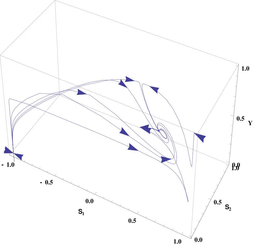 Figure 10
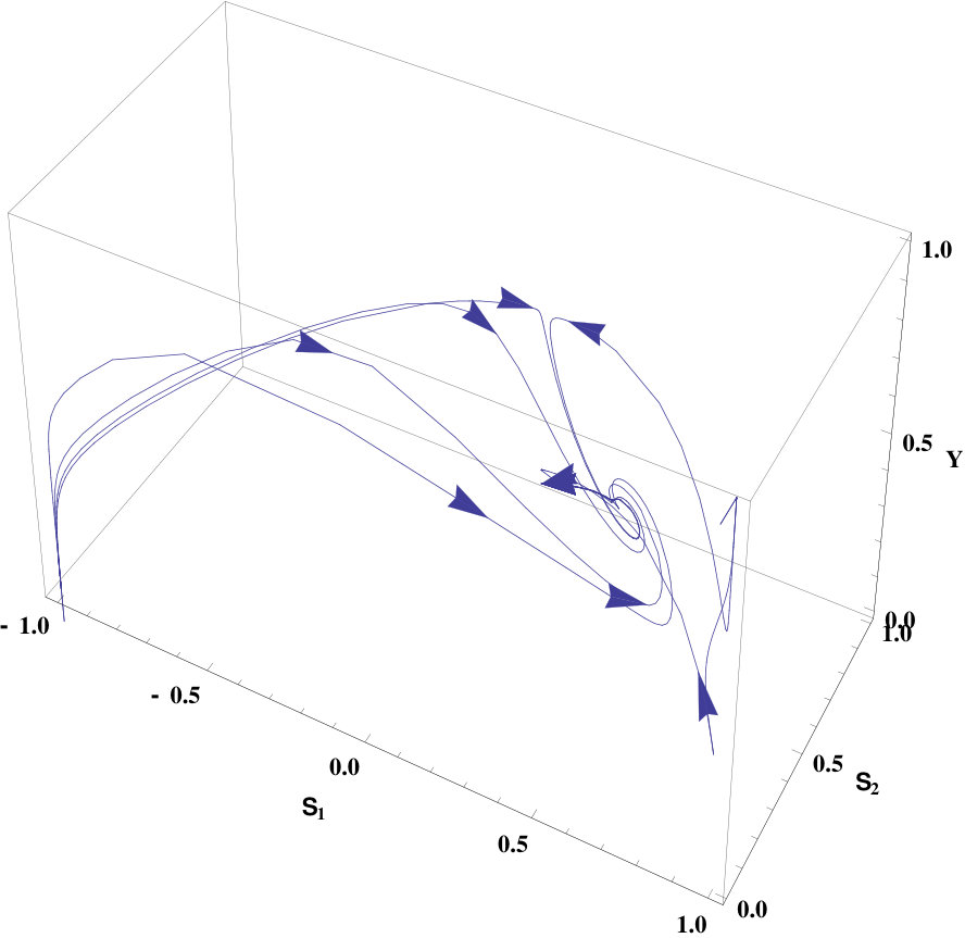 Figure 10
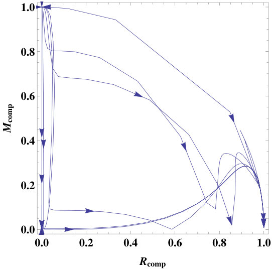 Figure 10
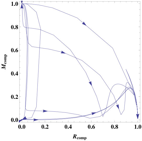 Figure 10
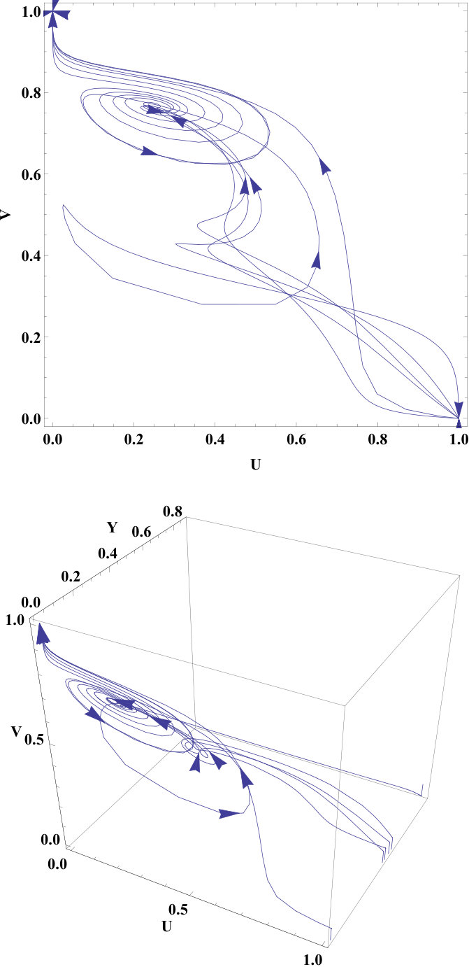 Figure 11
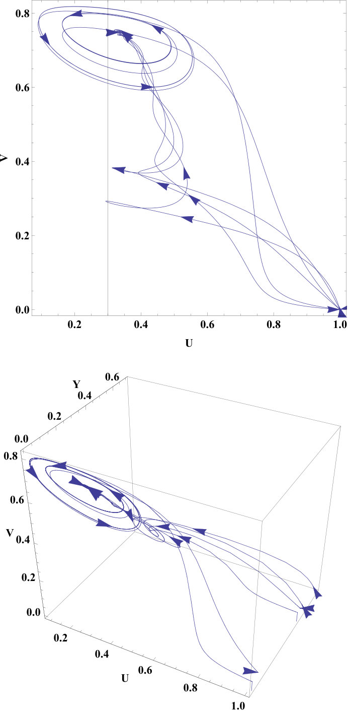 Figure 11
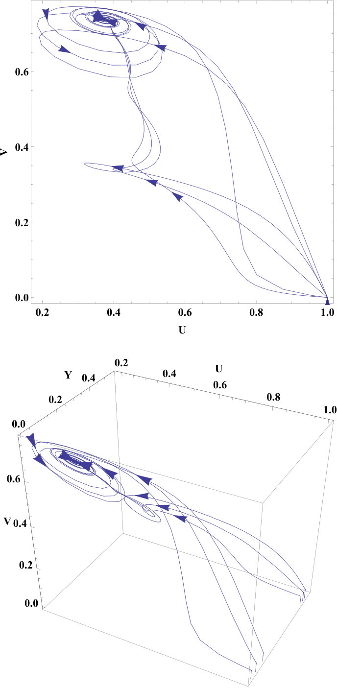 Figure 11
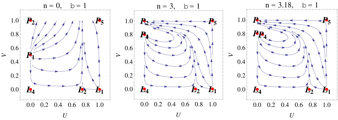 Figure 12
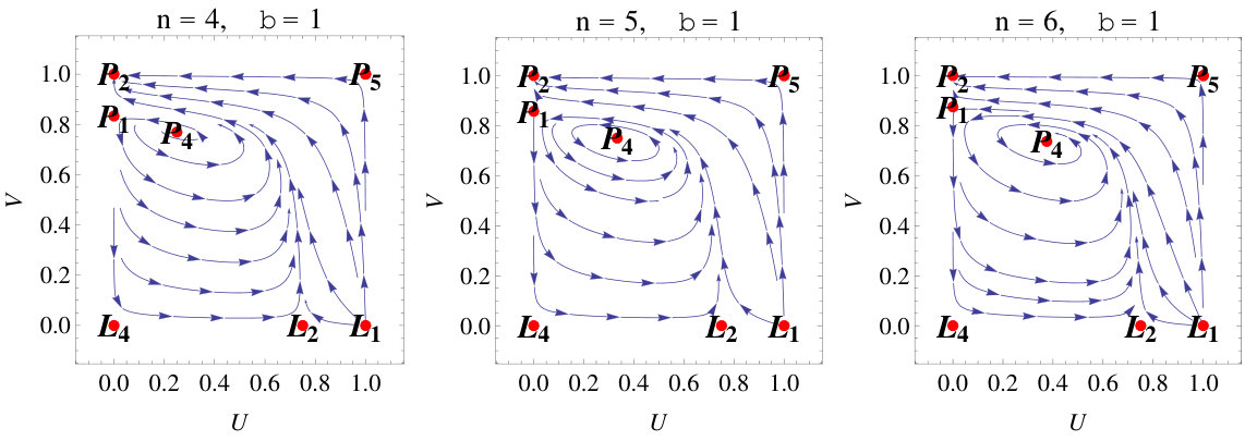 Figure 12
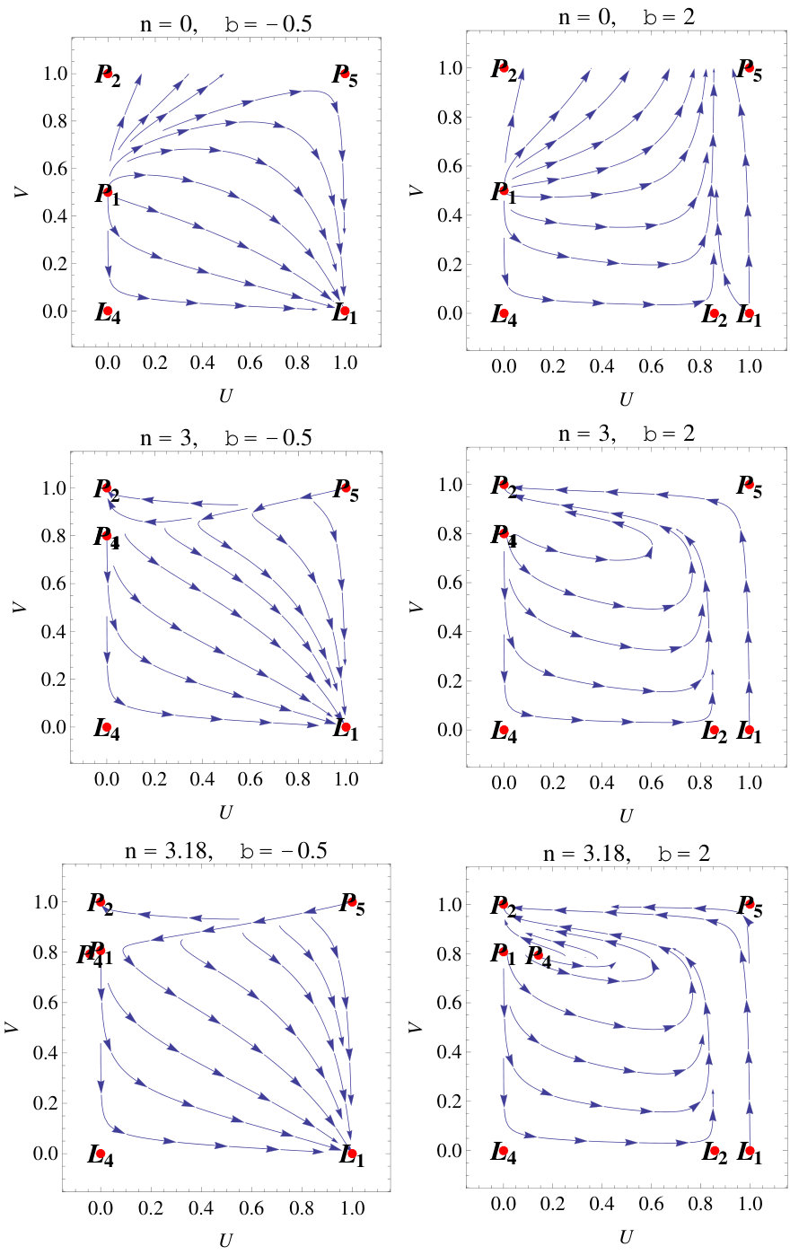 Figure 13
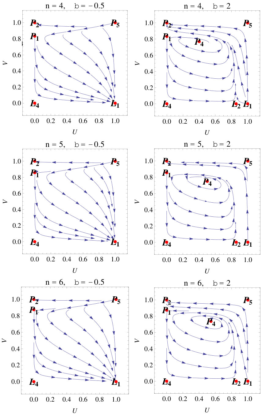 Figure 14
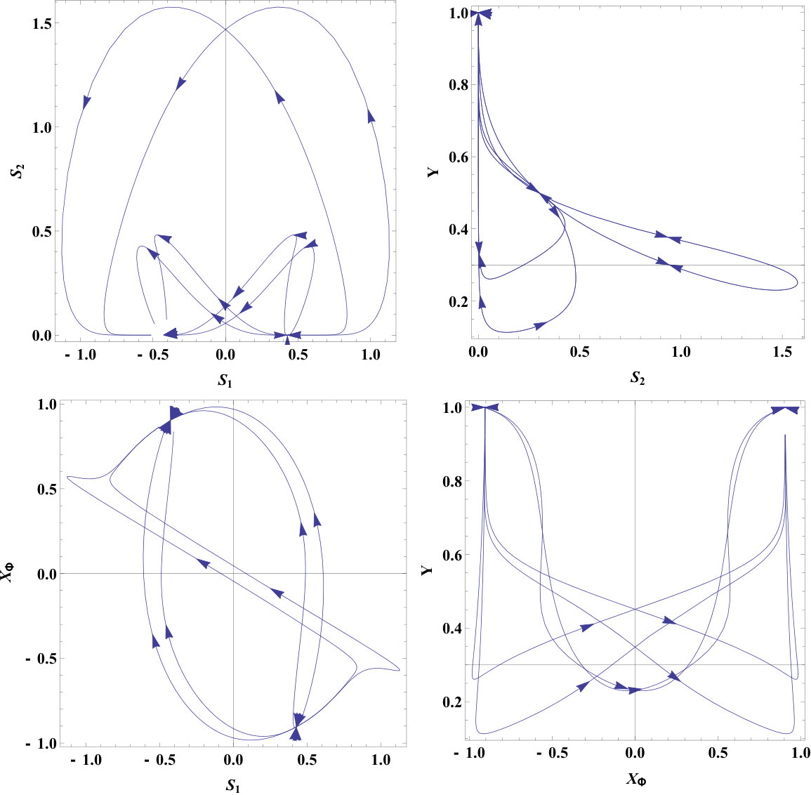 Figure 16
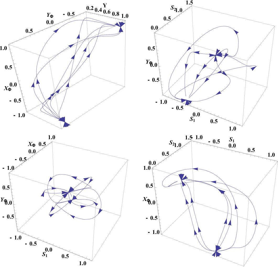 Figure 16
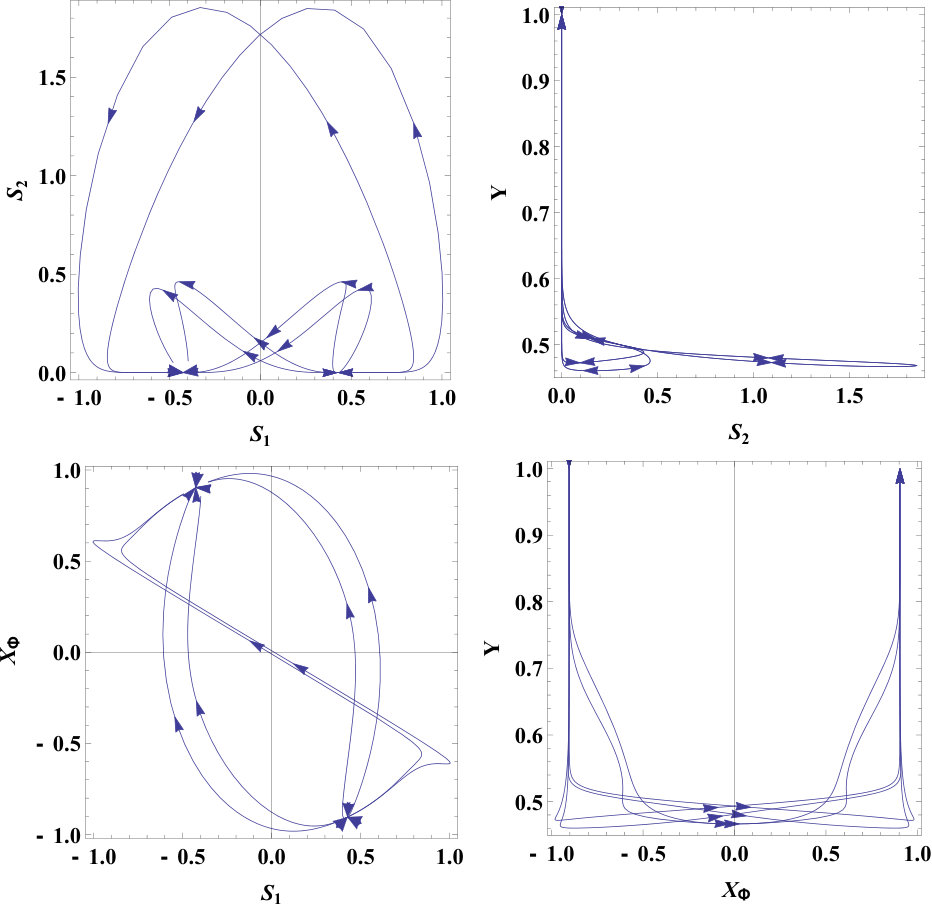 Figure 17
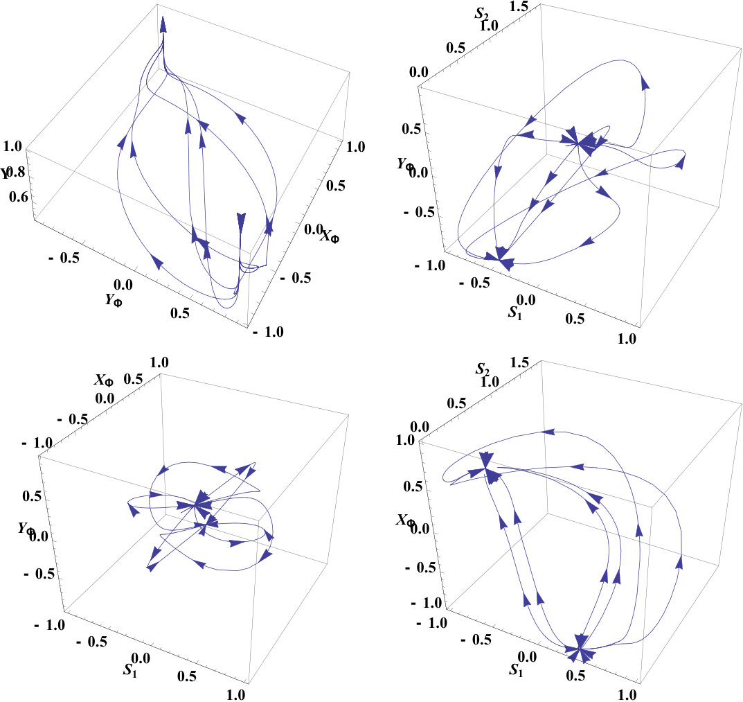 Figure 17
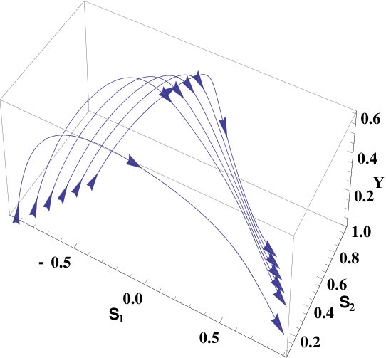 Figure 1
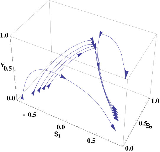 Figure 1
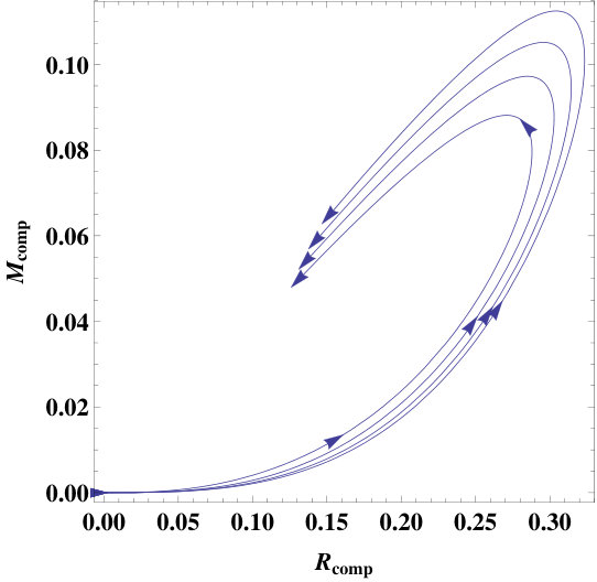 Figure 1
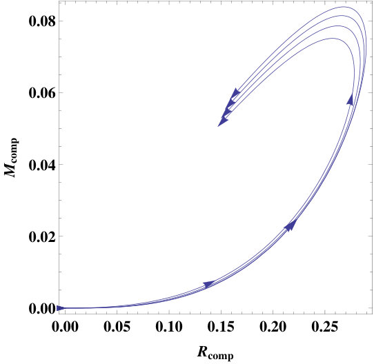 Figure 1
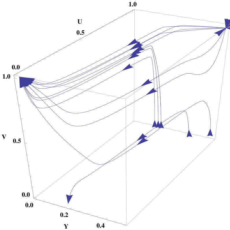 Figure 2
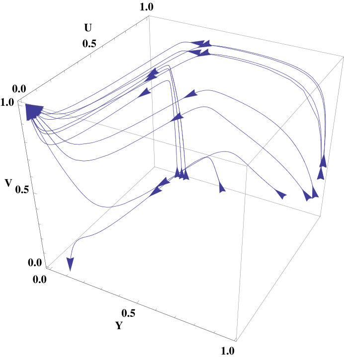 Figure 2
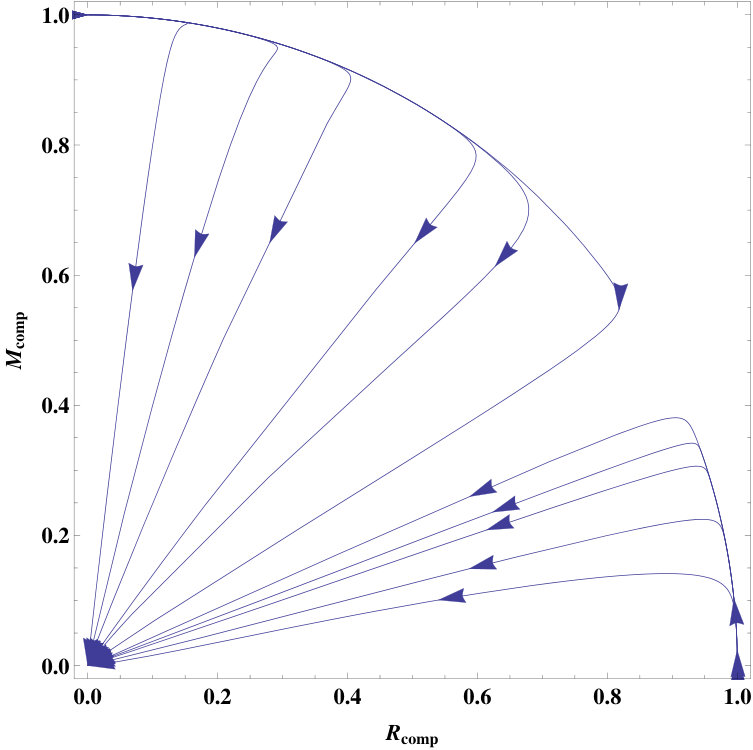 Figure 2
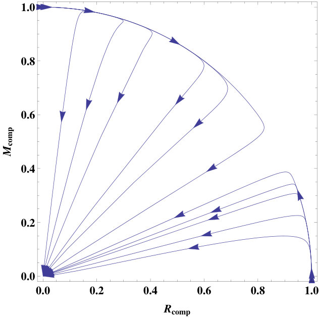 Figure 2
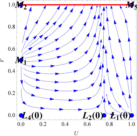 Figure 3
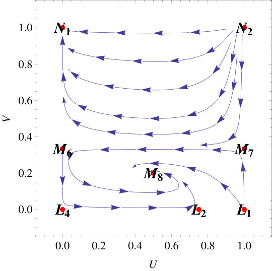 Figure 4
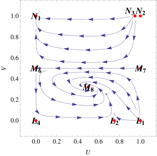 Figure 4
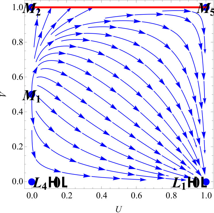 Figure 5
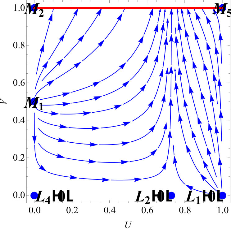 Figure 5
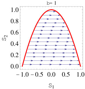 Figure 6
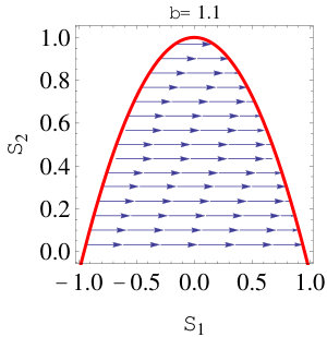 Figure 6
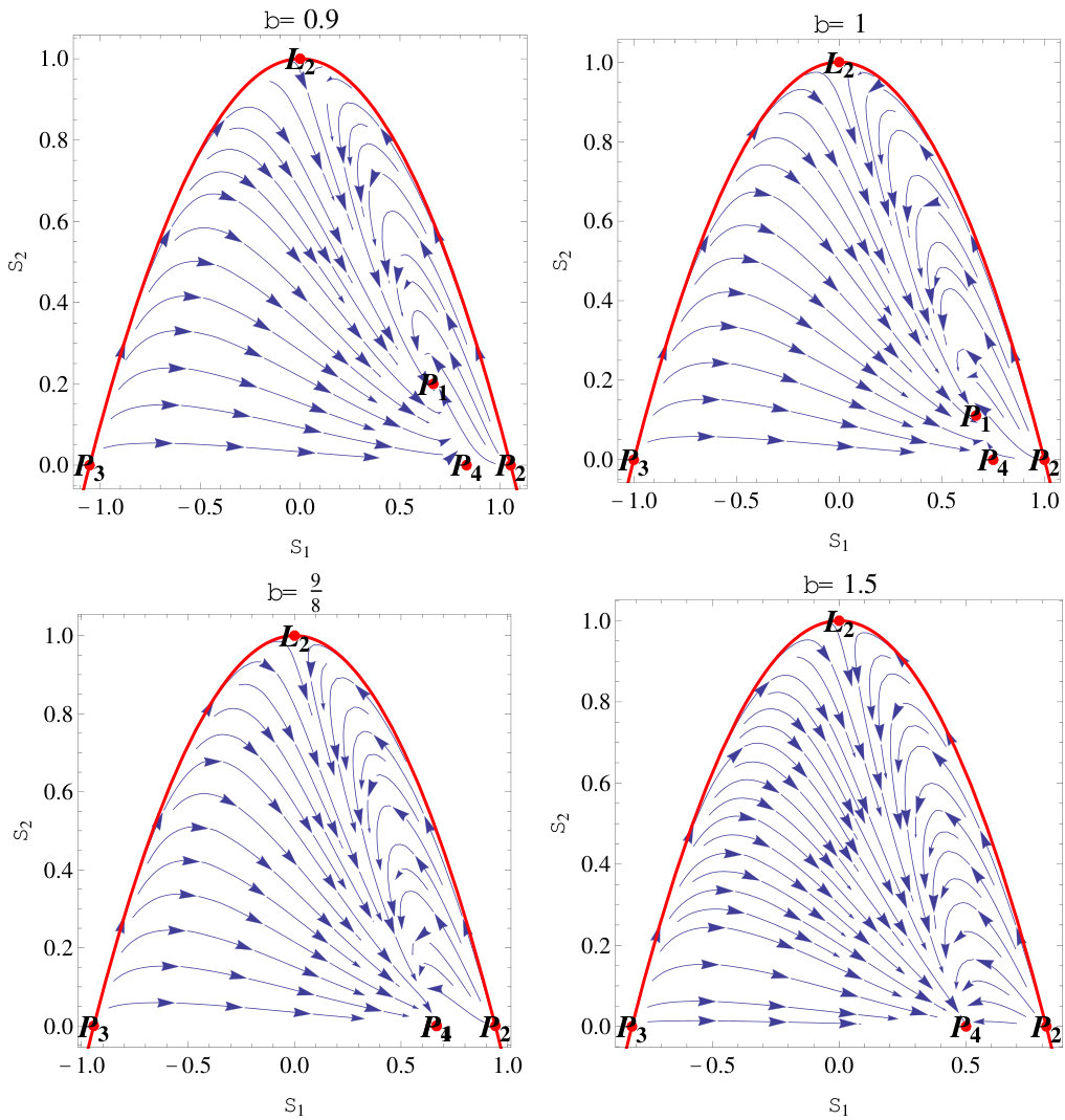 Figure 7
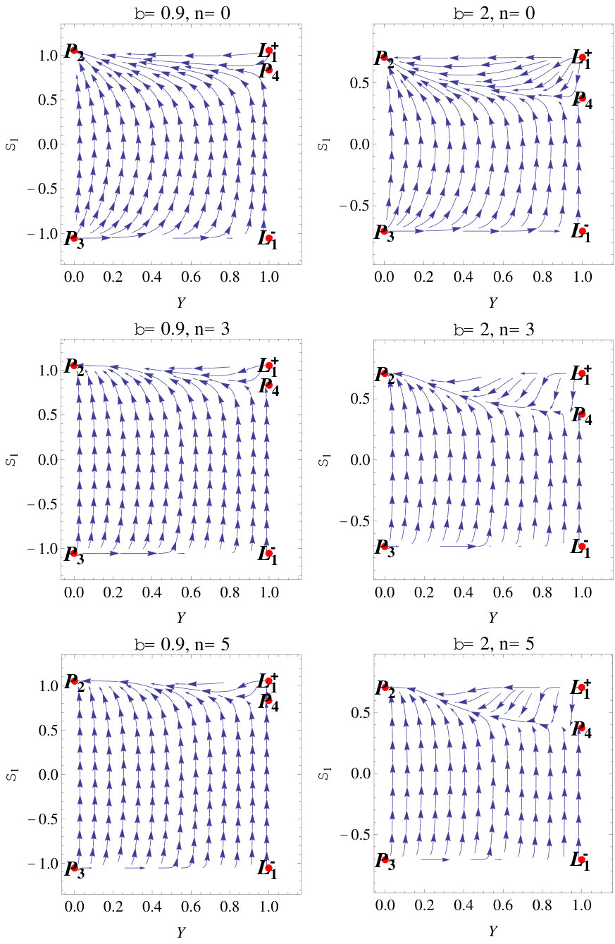 Figure 8
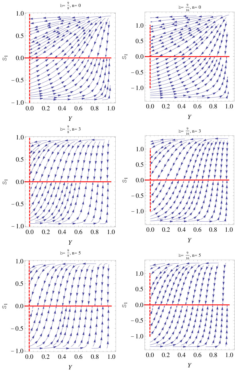 Figure 9
| Labels | Eigenvalues | Stability | |
| Normally hyperbolic. | |||
| Stable for . | |||
| Unstable for . | |||
| Saddle. | |||
| Saddle. | |||
| Source for | |||
| , | |||
| saddle otherwise. | |||
| Saddle. | |||
| Sink for | |||
| . |
| Labels | Eigenvalues | Stability | |
|---|---|---|---|
| Source. | |||
| Saddle. | |||
| Nonhyperbolic. | |||
| Saddle. | |||
| Nonhyperbolic. | |||
| Sink. | |||
| , | Saddle. | ||
| Sink. | |||
| Saddle. | |||
| Nonhyperbolic. | |||
| Saddle. | |||
| , | Saddle. | ||
| Saddle. |
| Labels | Eigenvalues | Stability | |
| Attractor for | |||
| , or | |||
| . | |||
| Source for | |||
| , or | |||
| . | |||
| . | Nonhyperbolic. | ||
| 2D unstable manifold for | |||
| . | |||
| 2D stable manifold for | |||
| , | |||
| or . | |||
| Saddle. | |||
| Saddle. | |||
| Nonhyperbolic. | |||
| Nonhyperbolic. | |||
| Nonhyperbolic for , | |||
| saddle otherwise. | |||
| Nonhyperbolic. | |||
| Nonhyperbolic. | |||
| 2D stable manifold for | |||
| , or | |||
| . | |||
| 2D unstable manifold for | |||
| . | |||
| Saddle. | |||
| Nonhyperbolic. | |||
| 2D stable manifold for | |||
| , or . | |||
| Nonhyperbolic. | |||
| Saddle. | |||
| Nonhyperbolic. | |||
| 1D unstable manifold. | |||
| . | Nonhyperbolic. | ||
| 1D unstable manifold for | |||
| , or | |||
| . | |||
| 1D stable manifold for | |||
| , or | |||
| . | |||
| Saddle. | |||
| Nonhyperbolic. | |||
| , | Nonhyperbolic. | ||
| Nonhyperbolic. |
| Labels | Eigenvalues | Stability | |
| for | Nonhyperbolic | ||
| saddle | |||
| saddle | |||
| Labels | Eigenvalues | Stability | |
| Attractor for | |||
| , or | |||
| . | |||
| Source for | |||
| , or | |||
| . | |||
| Nonhyperbolic | |||
| 2D stable manifold for | |||
| , or | |||
| . | |||
| 2D unstable manifold for | |||
| Nonhyperbolic. | |||
| Saddle. | |||
| Nonhyperbolic. | |||
| , | Nonhyperbolic. | ||
| 2D stable manifold for | |||
| , or | |||
| . | |||
| 2D unstable manifold for | |||
| . | |||
| Saddle. | |||
| Sink. | |||
| Saddle. | |||
| , | |||
| , | |||
| Stable spiral for . | |||
| Nonhyperbolic. | |||
| Nonhyperbolic. | |||
| 1D unstable manifold. | |||
| . | Nonhyperbolic. | ||
| 1D unstable manifold for | |||
| , or | |||
| , or | |||
| 1D stable manifold for | |||
| , or | |||
| . | |||
| Nonhyperbolic. | |||
| Saddle. | |||
| Nonhyperbolic. | |||
| 1D unstable manifold. | |||
| Nonhyperbolic. | |||
| , | Nonhyperbolic. | ||
| Nonhyperbolic. |
| Labels | Stability |
|---|---|
| Nonhyperbolic. 2D unstable (resp. stable) manifold for (resp. ). | |
| (resp. ) nonhyperbolic. 3D unstable (resp. stable) manifold for . | |
| (resp. ) is nonhyperbolic. 3D unstable (resp. stable) manifold for . | |
| saddle | |
| (resp. ) is nonhyperbolic with a 4D unstable (resp. stable) manifold for | |
| , or | |
| , or | |
| , or | |
| , or | |
| , or | |
| , or | |
| . | |
| saddle. | |
| nonhyperbolic. | |
| saddle. | |
| (resp. ) is nonhyperbolic with a 4D unstable (resp. stable) manifold for | |
| saddle. | |
| (resp. ) is a sink (resp. a source) for . They are saddle otherwise. | |
| saddle. | |
| (resp. ) is a source (resp. sink) for | |
| , or | |
| , or | |
| , or | |
| . | |
| saddle. | |
| For some choices of parameters, say , or , they are saddle. |
| Labels | Stability |
|---|---|
| (resp. ) is nonhyperbolic with a 3D unstable (resp. stable) manifold for | |
| , or | |
| , or | |
| , or | |
| . | |
| (resp. ) nonhyperbolic with a 3D stable (resp. unstable) manifold for | |
| , or | |
| , or | |
| , or | |
| , or | |
| , or | |
| , or | |
| , or | |
| , or | |
| . | |
| (resp. ) is nonhyperbolic with a 3D stable (resp. unstable) manifold for | |
| , or | |
| , or | |
| , or | |
| , or | |
| , or | |
| . | |
| (resp. ) is nonhyperbolic with a 3D unstable (resp. stable) manifold for | |
| , or | |
| , or | |
| , or | |
| , or | |
| . |
| Labels | Stability |
|---|---|
| Nonhyperbolic with a 2D unstable manifold (resp. stable) for (resp. ). | |
| (resp. ) is nonhyperbolic with a 3D unstable (resp. stable) manifold for . | |
| (resp. ) is nonhyperbolic with a 3D unstable (resp. stable) manifold for . | |
| saddle. | |
| (resp. ) is nonhyperbolic, with a 4D unstable (resp. stable) manifold for | |
| , or | |
| , or | |
| , or | |
| , or | |
| . | |
| saddle. | |
| Nonhyperbolic. | |
| saddle. | |
| saddle. | |
| (resp. ) is nonhyperbolic with a 4D unstable (resp. stable) manifold for . | |
| (resp. ) is a sink (resp. a source) for or a saddle otherwise. | |
| saddle. | |
| (resp. ) is a source (resp. a sink) for | |
| , or | |
| , or | |
| , or | |
| . | |
| It is a saddle otherwise. | |
| saddle. | |
| For they are saddle. |
| Labels | Stability |
|---|---|
| (resp. ) has a 3D stable (resp. unstable) manifold for | |
| , or | |
| , or | |
| , or | |
| , or | |
| , or | |
| , or | |
| , or | |
| , or | |
| , or | |
| . | |
| (resp. ) has a 3D unstable (resp. stable) manifold for | |
| , or | |
| , or | |
| . | |
| (resp. ) has a 3D stable (resp. unstable) manifold for | |
| , or | |
| , or | |
| . | |
| (resp. ) has a 3D unstable (resp. stable) manifold for | |
| , or | |
| , or | |
| , or | |
| , or | |
| , or | |
| . |
Peer Reviews
No public reviews on file for this paper yet. If you reviewed it on a platform where reviews are public (OpenReview, ICLR, NeurIPS, ICML), you can paste yours below so the community can read it here.
Videos
No videos yet. Explain this paper in a talk, walkthrough, or lecture? Add one.
Static Spherically Symmetric Einstein-æther models II: Integrability and the Modified Tolman-Oppenheimer-Volkoff approach
Genly Leon
Departamento de Matemáticas, Universidad Católica del Norte, Avda. Angamos 0610, Casilla 1280 Antofagasta, Chile.
A. Coley
Department of Mathematics and Statistics, Dalhousie University, Halifax, Nova Scotia, Canada B3H 3J5
Andronikos Paliathanasis
Institute of Systems Science, Durban University of Technology,
PO Box 1334, Durban 4000, Republic of South Africa.
Abstract
We investigate the existence of analytic solutions for the field equations in the Einstein-æther theory for a static spherically symmetric spacetime and provide a detailed dynamical system analysis of the field equations. In particular, we investigate if the gravitational field equations in the Einstein-æther model in the static spherically symmetric spacetime possesses the Painlevè property, so that an analytic explicit integration can be performed. We find that analytic solutions can be presented in terms of Laurent expansion only when the matter source consists of a perfect fluid with linear equation of state (EoS) . In order to study the field equations we apply the Tolman-Oppenheimer-Volkoff (TOV) approach and other approaches. We find that the relativistic TOV equations are drastically modified in Einstein-æther theory, and we explore the physical implications of this modification. We study perfect fluid models with a scalar field with an exponential potential. We discuss all of the equilibrium points and discuss their physical properties.
Contents
-
1.4 Tolman-Oppenheimer-Volkoff equation for relativistic star models
-
1.5 Integrability and modified Tolman-Oppenheimer-Volkoff formulation
-
3 Static spherically symmetric spacetime with a perfect fluid
-
3.1.2 Equilibrium points in the finite region of the phase space
-
3.1.3 Dynamical systems analysis based on the Newtonian homology invariants
-
3.2.2 Equilibrium points in the finite region of the phase space
-
3.2.3 Dynamical systems analysis based on the Newtonian homology invariants
-
4 Stationary comoving æther with perfect fluid and scalar field in static metric
-
4.1.2 Equilibrium points in the finite region of the phase space
-
4.2 Model 4: Perfect fluid with polytropic of state and a scalar field with an exponential potential
-
4.2.2 Equilibrium points in the finite region of the phase space
-
A.1 Equilibrium points of Model 1 at the finite part of the phase space
-
B.1 Equilibrium points of Model 2 at the finite part of the phase space
1 Introduction
Einstein-æther theory [1, 2, 3, 4, 5, 6, 7, 8, 9, 10, 11, 12] is an effective field theory preserving locality and covariance, and consists of General Relativity (GR) dynamically coupled to a time-like unit vector field (the æther), in which the local spacetime structure is determined by both the dynamical æther vector field and the geometrical metric tensor field [7]. Since a preferred frame is specified by the æther at each spacetime point, Lorentz invariance is broken spontaneously, more precisely it breaks the invariance under boosts. We note that every hypersurface-orthogonal Einstein-æther solution is a solution of the IR limit of (extended) Hořava gravity [13]; the relationship between Einstein-æther theory and Hořava-Lifschitz (HL) gravity is further clarified in [14].
Exact solutions and the qualitative analysis of Einstein-æther cosmological models have been presented by a number of authors, [15, 16, 17, 18, 19], with an emphasis on the impact of Lorentz violation on the inflationary scenario [6, 4, 5]. More recent developments of the HL theory were reviewed in [20], including universal horizons, black holes and their thermodynamics, gauge-gravity duality, and the possible quantization of the theory. HL cosmological scenarios were tested against new observational constraints in [21] using updated Cosmic Microwave Background, Type Ia supernovae, and Baryon Acoustic Oscillations cosmological data. It is known that cosmologically viable extended Einstein-æther theories are compatible with cosmological data [22].
1.1 Spherically symmetric models
The Einstein-æther field equations (FE) are derived from the Einstein-æther action [1, 3]. In such a model there will be additional terms in the FE due to the effects of the curvature of the underlying spherically symmetric geometry and from the stress tensor, , for the æther field (which depends on a number of dimensionless parameters ). In addition, because a FLRW limit is not required by the analysis, the æther field can be “tilted” with respect to the (perfect fluid) CMB rest frame, which provides additional terms in the matter stress tensor, (characterized by a “hyperbolic tilt angle”, , measuring the relative boost). It is anticipated that this tilt will decay to the future [23]. For example, (and consistent with the local linear stability analysis presented in [4]), at late times in a tilted (æther) Bianchi I cosmological model in which the initial hyperbolic tilt angle and its time derivative are sufficiently small [6].
The Einstein-æther parameters are dimensionless constants. In the case of spherical symmetry the æther is hypersurface orthogonal, so that the twist vanishes and can be set to zero without any loss of generality [7]. The spherically symmetric solutions of Einstein-æther theory are a subset of the solutions of Hořava gravity. In general the converse is not true, except when the solutions have a regular center [7]. The parameters also determine the effective Newtonian gravitational constant in the model, and consequently can be set to unity by an appropriate renormalization. The spherically symmetric model can thus be characterized by two non-trivial constant parameters. In GR . In the qualitative analysis that follows we shall assume values for the non-GR parameters compatible with all current constraints [7, 24]. In the case of a static vacuum there is a 3-parameter family of spherically symmetric solutions. In particular, when the æther is parallel to the Killing vector, which is referred as a “static æther”, a static vacuum solution is explicitly known [25].
Spherically symmetric static and stationary Einstein-æther solutions in which there is an additional (to GR) radial tilting æther mode are of physical importance, and a number of black hole and time-independent solutions are known [7, 24, 25, 26]. In general, the dynamics of the cosmological scale factor and perturbations in non-rotating neutron star and black hole solutions are very similar to those in GR. Although a fully nonlinear positive energy result has been demonstrated for spherically symmetric solutions at an instant of time symmetry [9], a thorough study of the fully nonlinear solutions has not yet been carried out.
1.2 Background
Recently spherically symmetric Einstein-æther cosmological models with a perfect fluid matter source have been studied [27], including FRW models [28], Kantowski-Sachs models [29, 19], and spatially homogenous metrics [30]. In all cases the matter source was assumed to include a scalar field which is coupled to the expansion of the æther field through a generalized exponential potential.
In order to perform a dynamical systems analysis [31] it is useful to introduce suitable normalized variables [32, 33, 34] to simplify the FEs, which also facilities their numerical study. In particular, we derive the equilibrium points of the algebraic-differential system by introducing proper normalized variables [18]. For every point the stability and the physical variables can be given.
The static spherically symmetric model with perfect fluid, first introduced in Section 6.1 of [18], has been investigated in [35] using appropriate dynamical variables inspired by [36]. In the reference [35] two of us have presented asymptotic expansions for all of the equilibrium points in the finite region of the phase space. We have shown that the Minkowski spacetime can be given in explicit spherically symmetric form [36] irrespective of the æther parameters. We have shown that we can have non-regular self-similar perfect fluid solutions (like those in [37, 38, 39]), self-similar plane-symmetric perfect fluid models, and Kasner’s plane-symmetric vacuum solutions [40]. We discussed the existence of new solutions related with naked singularities or with horizons. The line elements have been presented in explicit form. We also discussed the dynamics at infinity and presented some numerical results supporting our analytical results. Scalar field configurations in static spherically symmetric metrics were also included. The physical consequences of the models were discussed in [36, 41, 42], most of which are astrophysical rather than cosmological ones. Relativistic polytropic EoS were examined in [43] in Hořava gravity and in Einstein-æther theories with anisotropic fluid. Assuming viable analytic and exact interior solutions, there was found the equation of state (EoS) by a polynomial fit, not accurate enough to describe the relation between the density and the radial and tangential pressure, so that a correction of the relativistic polytropic EoS was needed to give a satisfactory fit.
The present research is the follow-up of reference [35]. Here we continue the investigation of static spherically symmetric Einstein-æther models. Particularly, we investigate the integrability of the FE and we present the Modified Tolman-Oppenheimer-Volkoff approach.
1.3 The Ablowitz, Ramani and Segur algorithm
The modern treatment of singularity analysis is summarized in the ARS algorithm (from the initials of Ablowitz, Ramani and Segur). There are three main steps to the algorithm, they are: (i) to determine the movable singularity, which should be a single pole, (ii) to determine the resonances which consist of the position of the integration constants in the Laurent expansion and (iii) perform the consistency test.
In order to demonstrate the application of the singularity analysis we consider the well-known Painlevè-Ince equation [44]:
[TABLE]
We substitute in the latter equation and we find the polynomial equation
[TABLE]
for which balance occurs if and consequence or . The requirement that there is a balance in the exponents is necessary in order for the function describes the behavior of the solution near the singularity. As we can see there are two coefficient constants which mean that there are two possible different solutions.
For the second step of the ARS algorithm we take
and we linearize around . We equate the remaining leading-order terms to zero and we find the values of the resonances, where for they are and while for the resonances are and . Because the resonances are rational numbers, we shall say that the Painlevè-Ince equation passes the second step of the ARS algorithm.
The final step is to write the solution in terms of a Laurent expansion, and for , the solution is given by the following partial Laurent expansion
[TABLE]
where is arbitrary, and denotes an integration constant of the solution; the position of the singularity is considered another integration constant. By replacing the latter Laurent expansion in the Painlevè-Ince equation, we obtain the coefficients
[TABLE]
Hence, we conclude that the Painlevè-Ince possesses the Painlevè property and passes the ARS algorithm.
The study of whether a nonlinear dynamical system posses the integrability property is essential in all physical theories. Indeed, by knowing that a given dynamical system is integrable we know that numerical trajectories/solutions describe real solutions of the dynamical system, while small changes in the initial conditions do not affect the main evolution of the system.
Usually we refer to a dynamical system as integrable when there exists a sufficient number of invariant functions which can be used to reduce the system into an algebraic equation and when it is thus feasible to write the explicit solution in terms of closed-form functions. However, in the context of the singularity analysis the concept of integrability is strict; that is, the solution of the dynamical system must be analytic apart from isolated movable pole-like singularities (or branch point singularities) so that the complex plane of the independent variable can be divided into sections and in each section the solution is analytic. Because of this latter criteria, the free parameters of the theory are constrained in order for the dynamical system to possess the Painlevè property. This is essentially only a mathematical criterion and does not necessarily provide physical properties of the system.
For other values of the free parameters, where the dynamical system does not pass the singularity analysis, other methods for the determination of the conservation laws should be used in order to analyze the integrability of the system.
1.4 Tolman-Oppenheimer-Volkoff equation for relativistic star models
The Tolman-Oppenheimer-Volkoff approach for a relativistic star model is based on the equations (in units where ):
[TABLE]
where, , , are the density, the pressure, and the mass enclosed in a sphere of radius . Equation (5a) is the well-known Tolman-Oppenheimer-Volkoff equation. is the gravitational potential. The last equation is decoupled, and we obtain a reduced 2D system of differential equations provided an EoS is given.
Now we discuss some particular models. Following the reference [45], a model with the isothermal equation of state was studied. By utilizing the new variables
[TABLE]
where denotes the Misner-Sharp mass [46], and introducing , and the new radial variable the field equations can be cast as [45]:
[TABLE]
Defining
[TABLE]
the Lotka-Volterra model is obtained
[TABLE]
In [45] it was proven that the above system is Liouville-integrable if and only if , where by Liouville-integrable is it understood that a system of polynomial differential equations have first integrals given by elementary functions or integrals of elementary functions (that is, functions expressed in terms of combinations of exponential functions, trigonometric functions, logarithmic functions or polynomial functions). In the special cases (cosmological de Sitter solution) and , the resulting system can be expressed as Abel equations of second order that are exactly solvable.
Another important EoS model leads to ideal polytropes stars [47]:
[TABLE]
where is the so-called polytropic index. Is it well-known that the value is a bifurcation value that separates two regimes [47]:
: corresponding to “gas spheres” of infinite extension;
- 2.
: corresponding to finite stars with boundary.
Therefore, it is convenient to consider variables that can distinguish between configurations with infinite extensions from that of finite extension and, similarly, that distinguish between finite and infinite masses.
For fluid spheres of mass and radius we have the universal scaling (--relation) [48]:
[TABLE]
where is a constant depending on the EoS, where it is presumed that and are finite. This motivates the following definition of compact variables:
[TABLE]
which are both finite when and are finite, and as , and as . Furthermore, the circle corresponds to any solution with , and . These variables are closely related (and have an analogous physical interpretation) to the variables used in [48]:
[TABLE]
where and are typical values of radii and mass. That is as , and as . The only difference is that in the second formulation the case of infinite mass and infinite radius corresponds to the point in the vs diagram, instead of the whole or part of the circle in our formulation (but they share the same qualitative features).
In reference [48]some relevant mass-radius theorems for relativistic spherically symmetric static perfect fluid models were proved. In particular, a general class of asymptotically polytropic EoS, where the relevant parameters and are defined as follows, was considered:
[TABLE]
where and are the density and the pressure of the fluid and , the so-called pressure variable, is a dimensionless continuous function for , strictly monotonically increasing and sufficiently smooth on with and [48]. Was also considered an EoS such that is a continuous function for , with continuous first order derivative for , and such that
[TABLE]
Here , and are constants that satisfy . Additionally, it is assumed
[TABLE]
The relevant Mass-radius theorem for relativistic spherically symmetric static perfect fluid models states (Theorems: 5.1, 5.2, 5.3, 5.4 of [48]):
All regular solutions have infinite masses and infinite radii if and .
- 2.
All regular solutions with have finite mass and radii if and .
- 3.
All regular and non-regular perfect fluid solutions have finite radii and masses if (i.e., ).
- 4.
For , and for sufficient high central pressures (i.e., when ), the mass-radius - diagram exhibits a spiral structure, with and given by the formulas (29) and (30) of [48].
As a consequence, for relativistic static spherically symmetric perfect fluid models with exact polytropic EoS, all regular solutions possess finite and for (). All regular solutions with small central pressures have finite extent when (). In the case of asymptotic polytropic EoS (in the sense discussed above), the result is that all regular solutions with possess finite and [48].
1.5 Integrability and modified Tolman-Oppenheimer-Volkoff formulation
In order to prove that there actually exist solutions, the integrability of the system should be established [49, 50, 51, 52, 53, 54, 55]. We first study the integrability of static spherically symmetric spacetimes in Einstein- æther gravity with a matter source of the form of a perfect fluid with EoS . The governing equations for such a spacetime form an algebraic-differential system of first order which can be written as system of second-order differential equations with fewer independent variables by utilizing the ARS (Ablowitz, Ramani and Segur) algorithm [56]. We first show that the system passes the singularity test, which implies that they are integrable. Additionally, we consider a polytropic EoS , and we extend the analysis by adding a scalar field with an exponential potential.
Specifically, we investigate if the gravitational FE in the Einstein-æther model in the static spherically symmetric spacetime posses the Painlevè property (so that an analytic explicit integration can be performed). In order to perform such an analysis we apply the classical treatment for the singularity analysis which is summarized in the ARS algorithm. As far as the dynamical system with only the perfect fluid is concerned, we show that the FE are integrable and we write the analytic solution in terms of mixed Laurent expansions. We show that if the scalar field is not present, and assuming that the perfect fluid has the EoS , the system passes the singularity test, which implies that it is integrable (in a similar way to what has been done for Kantowski-Sachs Einstein-æther theories in [19]). That is, in the case of the static spherically symmetric spacetime with a perfect fluid there always exist a negative resonance which means that the Laurent expansion is expressed in a Left and Right Painlevé Series because we integrate over an annulus around the singularity which has two borders [57]. On the other hand, in the presence of a scalar field, or when the EoS of the perfect fluid is polytropic , the FE do not pass the Painlevè test. Therefore, they are not integrable.
It is worth mentioning a few technicalities. First, we have to choose coordinates that can make the calculations simpler. Furthermore, since we know that the full system is, in general, non-integrable (including simpler models with realistic matter for neutron star solutions or for vacuum solutions in the context of modified gravity) we have to use techniques that do not involve actually solving the FE. The local semi-tetrad splitting [58] allows us to recast the FE into an autonomous system of covariantly defined quantities [59, 60]. This enables us to get ride of all the coordinate singularities that may appear because of badly defined coordinates. In addition, the autonomous systems can be simplified further by incorporating Killing symmetries of the spacetimes. For studying the integrability of the FE we combine the ARS method [19], Lie/Noether symmetries [61, 62] and Cartan symmetries [63]. In this research we use the ARS method.
One special application of interest is to use dynamical system tools to determine the conditions under which stable stars can form. By using the Tolman-Oppenheimer-Volkoff (TOV) approach [37, 38, 39], the relativistic TOV equations are drastically modified in Einstein-æther theory, and we can explore the physical implications of this modification. This approach to studying static stars uses the mass and pressure as dependent variables of the Schwarzschild radial coordinate. The resulting equations are however not regular at the center of the star, and a regularizing method for analyzing the solution space is required. In the relativistic and Newtonian case the resulting equations of the regularizing procedure are polynomial, and therefore they are regular. However, for the non-relativistic case the main difficulty is that the resulting system is rational. However, we are able to find some analytical results that are confirmed by numerical integrations of 2D and 3D dynamical system in compact variables, to obtain a global picture of the solution space for a linear EoS, that can visualized in a geometrical way. This study can be extended to a wide class of EoS. For example, we study the case of a polytropic EoS: in the static Einstein-æther theory, by means of the so-called -formulation given by the model (93). For the model of [41] is recovered.
The paper is organized as follows. In Section 2 we give the basic definitions of Einstein-æther gravity. In Section 3 we study static spherically symmetric spacetime with a perfect fluid with a linear EoS (Subsection 3.1) and with a polytropic EoS (Subsection 3.2). For each choice of the EoS for the perfect fluid we provide i) a singularity analysis and integrability analysis of the FE; ii) a local stability analysis of the equilibrium points in the finite region of the phase space, using the formulation, that takes advantage of the local semi-tetrad splitting, iii) a local stability analysis of the equilibrium points at infinity (when ) using the dominant quantities to create compact variables; and finally iv) we present a dynamical systems analysis based on the Newtonian homology invariants, -formulation, that makes use of the TOV formulation of the FE. As we see, are obtained as a particular case the results for relativistic and Newtonian stellar models. For the TOV formulation of the Einstein-æther modification, the main difficulty is that although the non-regular nature of the equations at the center is overcome using Newtonian homology-like invariants, the resulting equations are rational (includes radicals) and are more difficult to analyze as compared with the local semi-tetrad splitting formulation. Finally, we investigate in Section 4 a stationary comoving æther with a perfect fluid with both linear and polytropic EoS and a scalar field with exponential potential in a static metric. We find that the models do not have the Painlevè property. Therefore, they are not integrable. We investigate the stability of the equilibrium points using the local semi-tetrad splitting formulation due to their advantages over the Newtonian homology-like invariants formulation in the Subsections 4.1.2 (for the linear EoS) and 4.2.2 (for polytropic EoS). Finally in Section 5 we discuss our results and draw our conclusions. In A and in B we present a detailed stability analysis of the equilibrium points for perfect fluid models (with linear or polytropic EoS, respectively) using the four approaches, i) - iv) previously described. In C and in D we present a detailed stability analysis of the equilibrium points when the matter content consists on a perfect fluid and a scalar field with an exponential potential.
2 Einstein-æther Gravity
The Einstein-æther Action Integral is given by [7, 8]
[TABLE]
where is the Einstein-Hilbert term, is the term which corresponds to the matter source and
[TABLE]
corresponds to the æther field. is a Lagrange multiplier enforcing the time-like constraint on the æther [9], for which we have introduced the coupling [7]
[TABLE]
which depends upon four dimensionless coefficients . Finally, is the normalized time-like vector (observer) in which .
Variation with respect to the metric tensor in (16) provides the gravitational FE
[TABLE]
in which is the Einstein tensor, corresponds to , and is the æther tensor [64]
[TABLE]
and variation with respect to the vector field and the Lagrange multiplier gives us
[TABLE]
[TABLE]
and the compatibility conditions
[TABLE]
where is the projective tensor where . We shall use the equation (22) as a definition for the Lagrange multiplier, whereas the second equation (23) leads to a set of restrictions that the æther vector must satisfy.
The energy momentum tensor of a matter source of the form of a perfect fluid (which includes a scalar field) with energy density , and pressure , in the 1+3 decomposition with respect to , is
[TABLE]
where is the density and is the pressure of the perfect fluid, respectively.
For simplicity, in the following we introduce the constants redefinition .
3 Static spherically symmetric spacetime with a perfect fluid
We consider a static spherically symmetric spacetime with line element
[TABLE]
where we have fixed the spatial gauge to have , and .
The FE are [18]:
[TABLE]
Furthermore, there exists the constraint equation
[TABLE]
From (26c) and (26d) we have that , where the prime ′ denotes a derivative with respect . By substituting into (26a), and (26b) we find a system of two second-order ordinary differential equations,
[TABLE]
while (27) becomes
[TABLE]
In order to apply Tolman-Oppenheimer-Volkoff approach (recall that we use units where ) we use a coordinate change to write the line element as
[TABLE]
and define
[TABLE]
where is the gravitational potential, denotes the mass up to the radius , with range , which in the relativistic case is defined by
[TABLE]
such that (in the relativistic case)
[TABLE]
Now we will calculate , and in the Einstein-æther theory and compare with the relativistic TOV equations. By definition
[TABLE]
Equation (34a) leads to the definition
[TABLE]
Taking derivative with respect to in both sides of (35) and using Eqs. (26a) and (31) we obtain
[TABLE]
On the other hand, the identity
[TABLE]
can be written as
[TABLE]
Equations (36), (38) have two solutions for and . We consider the branch
[TABLE]
Taking the limit in the Eqs. (39) we obtain the proper general relativistic equations (5).
We have to consider the reality conditions:
[TABLE]
or
[TABLE]
For the analysis we have to specify the equation of state, at least on implicit form . One can be interested in determine conditions on which stable stars can form. The set of equations (39), determine the star’s structure and the geometry in the static spherically symmetric Einstein-æther theory for a perfect fluid. Equation (39a) is a modification of the well-known Tolman-Oppenheimer-Volkoff equation for relativistic star models.
3.1 Model 1: Linear equation of state
For the equation of state for the perfect fluid we consider that , with .
3.1.1 Singularity analysis and integrability
In this section we use the line element (25). Then, by introducing the radial rescaling , such that as and as , we obtain the equations
[TABLE]
while (27) becomes
[TABLE]
where ∗ means derivative with respect to .
Next, we apply the ARS algorithm and we find that the dominant terms are111We have taken the position of the singularity to be at zero. where
[TABLE]
For the resonances we have that
[TABLE]
where
[TABLE]
Furthermore, as for the resonance is negative, the Laurent expansion is a Left-Right Painlevé Series. Importantly, for the singularity analysis to succeed the resonances must be rational numbers.
Consider the special case with , which gives the resonances Hence the solution is given by
[TABLE]
[TABLE]
For , after we replace the solution (45), (46) in (28a) we find that the coefficient constants are
[TABLE]
[TABLE]
[TABLE]
[TABLE]
where are the two constants of integration. The third constant of integration is the position of the singularity while the fourth constant of integration appears in the next coefficients. Furthermore, from (41) we have the constraint for the constants of integration, .
For , we find the coefficients (47), (48),
[TABLE]
[TABLE]
[TABLE]
where again are two constants of integration.
From this analysis we performed the consistency test and we showed that the FE (40a)-(41) pass the singularity analysis and form an integrable system for values of the free parameters for which the resonances are rational numbers.
3.1.2 Equilibrium points in the finite region of the phase space
In this section we consider the line element (25), with the definition (). For the dynamical systems formulation we introduce the phase space variables
[TABLE]
Assuming that the energy density and the pressure are both non-negative we obtain , where we have attached the boundaries and . On the other hand, by definition.
The relation between the gravitational potential , and the matter field is given by
[TABLE]
Hence,
[TABLE]
where is a freely specifiable constant corresponding to the freedom of scaling the time coordinate in the line element. This in turn reflects the freedom in specifying the value of the gravitational potential at some particular value of . Matching an interior solution with the exterior Schwarzschild solution at the value where the pressure vanishes, however, fixes this constant. Using the variables we obtain the dynamical system
[TABLE]
where we have defined the new radial coordinate by
[TABLE]
We have the additional equation
[TABLE]
which implies that is an invariant subset. Thus, since , we have from (54b) that for . Hence, system (57) defines a flow on the (invariant subset) phase space:
[TABLE]
Finally, from the definitions of and we obtain the auxiliary equations
[TABLE]
The first equation implies that the sign of is invariant. Thus, we can choose and then, the direction of the radial variable is well defined. The last two equations lead
[TABLE]
which relates the variable and the logarithmic derivative of the gravitational potential [41]. The third equation implies that the function , defined by
[TABLE]
is monotone for , and . Additionally, the function is monotonic for . Together with other monotone functions defined on the boundary subsets, this implies that all of the attractors for (when the phase space is compact) are equilibrium points on the boundary sets , and which are invariant for the flow of (57).
In the table 1 the equilibrium points and the corresponding eigenvalues of the dynamical system (57) are presented (see A.1 for details; the behavior at infinity is discussed in A.2).
We have the -relation [48]
[TABLE]
where denotes the Misner-Sharp mass [46]. Using the equations (3.1.2), we can define the compact variables
[TABLE]
which depends only of the phase-space variables . Evaluating numerically the expressions at the orbits of the system (57), we can see whether the resulting model leads to finite radius and finite mass (see discussion in Section 1.4, that follows from reference [48]).
In table 1 we present the equilibrium points and the corresponding eigenvalues of the dynamical system (57).
In the Figure (1(a)) are shown some orbits of the system (57) on the plane for . In the Figure (1(b)) are shown some orbits of the system (57) on the plane for . In the Figures 1(c) and 1(d) is presented how the compact variables , defined by (96) varies along the orbits of (57) for different choices of the parameters.
3.1.3 Dynamical systems analysis based on the Newtonian homology invariants
In this section we use dynamical system tools to determine conditions under which stable stars can form. We start with the set of equations (39), which determine the star’s structure and the geometry in the static spherically symmetric Einstein-æther theory for a perfect fluid. Equation (39a) is a modification of the well-known Tolman-Oppenheimer-Volkoff equation for relativistic star models. The idea is to construct a 3D dynamical system in compact variables and obtain a global picture of the solution space for a linear equation of state, that can be visualized in a geometrical way. This study can be extended to a wide class of equations of state. We therefore introduce the - formulation as follows: we define
[TABLE]
that are obtained by a compactification of the so- called Newtonian homology invariants [65]
[TABLE]
where and are the density and pressure of the background fluid. The homology invariants are defined in [65] by
[TABLE]
The relation between the variables and used in paper [35] are:
[TABLE]
Furthermore, the relation between the variables and are
[TABLE]
To use the dynamical system tools, we have to define a new independent variable by
[TABLE]
Under the conditions , it follows that the variables are compact. The new variable has the same range as , i.e., as and as .
Assumptions of the positive energy density, pressure and mass, with the condition , leads to the inequalities:
[TABLE]
Since we are dealing with relativistic models the condition has to be satisfied, so that we have
[TABLE]
As a first step before to studying the full system we consider the case , which corresponds to the equations of GR (5). We compare our results with the results found in [41, 48].
General Relativity case ()
Using the equations (5), and considering the time derivative (72), we obtain the dynamical system
[TABLE]
We have included the boundary subsets , together with the “static surface” . From (75c) follows that the variable is monotonically decreasing and all the orbits ends at the Newtonian boundary subset .
The equilibrium points and curves of equilibrium points of (75) are summarized in table 2 (see details in the A.3).
We have the useful -relation
[TABLE]
where defines the Misner-Sharp mass [46]. Using the equations (3.1.3), we can define the compact variables
[TABLE]
which depends only of the phase-space variables , and evaluated along the orbits of the system (75), are useful to analyze whether the resulting model leads to finite radius and finite mass.
In the table 2 is summarized the information of the equilibrium points and the corresponding eigenvalues of the dynamical system defined by equations (75). In the Figure 2 it is presented how the compact variables , defined by (77), vary along the orbits of (75), and the attractor solutions has finite mass and finite radius. Additionally, are presented some orbits of the system (75).
Low pressure regime (The Newtonian subset )
We now consider the low pressure regime, also referred as the “Newtonian subset” , which is of great importance for relativistic stars. The stability analysis below is restricted to the dynamics onto the invariant set , and the stability along the -axis is not taken into account.
The evolution equations are given by
[TABLE]
defined on the phase plane
[TABLE]
The equilibrium (curves of equilibrium) points in this invariant set are:
, which is an endpoint of the line with described in the previous section. The eigenvalues are , such that it is a source. 2. 2.
, which is an endpoint of the line with described in the previous section. The eigenvalues are , such that it is a saddle. 3. 3.
, which is an endpoint of the line with described in the previous section. The eigenvalues are , such that it is a saddle. 4. 4.
. The eigenvalues are . It it a sink. 5. 5.
. The eigenvalues are , such that it is a source. 6. 6.
. The eigenvalues are , such that it is a non-hyperbolic equilibrium point (it is contained in the attractor line previously described). 7. 7.
. The eigenvalues are . Hence, it is a non-hyperbolic equilibrium point (it is contained in the attractor line previously described).
In the Figure 3 are presented some streamlines of the system (78). The solid (red) line denotes the line , which is a local attractor. The straight vertical line connecting with the line is the so-called Tolman orbit (associated to the positive eigenvalue of , the so-called Tolman point).
High pressure regime ()
In the limit , the equations becomes
[TABLE]
The equilibrium points in this regime are
: , with eigenvalues . Local source. 2. 2.
: , with eigenvalues . Saddle. 3. 3.
: , with eigenvalues . Saddle. 4. 4.
: , with eigenvalues . Exists for . Saddle. 5. 5.
: . The eigenvalues are . Exists for . Saddle. 6. 6.
: , with eigenvalues
. Exists for . It is an stable node for . Stable spiral for . 7. 7.
: , with eigenvalues . This point is over the static surface. It can be a local attractor on the invariant set . 8. 8.
: , with eigenvalues . This point is over the static surface. It is a local source for . It is a saddle for . 9. 9.
: , with eigenvalues . Exists for . This point is over the static surface. It is a local source for .
In the Figure 4 are presented some streamlines of the system (80) which corresponds to the high pressure regime. In this regime, the solution , that has finite mass and radius, is a local attractor. The line acts as a separatrix. The orbits above this line are attracted by .
Einstein-æther modification
In this case the dynamical system is given by
[TABLE]
where
[TABLE]
Observe that . In the limit , we obtain an equivalent dynamical system to (75).
The dynamical system (81) is defined on the bounded phase space
[TABLE]
From the equation (81c) we determine the invariant sets . In the table 3 are presented the equilibrium points and the corresponding eigenvalues and stability conditions of the dynamical system (81). See the details of the analysis in A.4. In the analysis of the solution space we identify the low pressure regime (so-called, the Newtonian subset), which corresponds to the invariant set .
Low pressure regime (The Newtonian subset)
We now consider the “Newtonian subset” , where the evolution equations are given by
[TABLE]
defined on the phase plane
[TABLE]
The equilibrium (curves of equilibrium) points in the invariant set are:
. The eigenvalues are , such that it is a source. 2. 2.
. The eigenvalues are , such that it is a non-hyperbolic equilibrium point (it is contained in the attractor line described below). 3. 3.
. The eigenvalues are . Hence, it is a non-hyperbolic equilibrium point (it is contained in the attractor line described below). 4. 4.
. The eigenvalues are , such that it is a source for and a sink for . 5. 5.
, which is an endpoint of the line described in the previous section. It exists for . The eigenvalues are , such that it is a saddle. 6. 6.
, which is an endpoint of the line described in the previous section. The eigenvalues are , such that it is a saddle. 7. 7.
The line . The eigenvalues are . This line is normally hyperbolic and due to the non-zero eigenvalue is negative it is a sink.
We see that the main difference with respect the case previously discussed is in that can be an attractor for , see figure 5(a). In the Figure 5(b) it is presented the case for , essentially the same behavior as for the model (78).
3.1.4 Physical discussion
By using the formulation, we have deduced the system (57). In this model the line of equilibrium points is normally hyperbolic. The sector of with is stable, whereas, the sector of with is unstable. Another important equilibrium point is ; a sink for .
For the low pressure regime governed by the equations (78), the line is a local attractor. The Tolman orbit is the one that connects the Tolman point with the line , and it is associated with the positive eigenvalue of . When (Einstein-æther modification), can be an attractor, whereas for , we essentially have the same behavior as for the model (78).
In the high pressure regime and for and , it is obtained the system of differential equations (80), for which the attractor is : . It is stable node for ; Stable spiral for . This point represents physical solutions that have finite mass and radius.
Implementing the procedure described in A.2 (which applies for ), we conclude that there are not physically relevant equilibrium points at infinity, apart from the source point that has , finite and . This solution corresponds to finite and . That is, where is the radial coordinate. Then implies that where is the central pressure (at ). As , the pressure increases as the solutions move away from this point.
3.2 Model 2: Polytropic equation of state
We use the line element
[TABLE]
where is the gravitational potential, is the usual Schwarzschild radial parameter, and is a dimensionless (under scalar transformations) freely specifiable function, that defines the spatial radial coordinate . The choice corresponds to isotropic coordinates and the function can viewed as a relative gauge function with respect to the isotropic gauge [41].
The FE are [18]:
[TABLE]
where for any function , we define , and
. Furthermore there exists the constraint equation
[TABLE]
Choosing a new radial coordinate such that
[TABLE]
the system (87) becomes
[TABLE]
with restriction (88). The above equations transforms to eqs. (A.3) in [41] for the choice , under the identifications . We consider a polytropic equation of state .
3.2.1 Singularity analysis and integrability
The FE does not pass the Painlevè test, and therefore they are not integrable.
3.2.2 Equilibrium points in the finite region of the phase space
For the dynamical system’s formulation we introduce the variables
[TABLE]
Assuming that the energy density and the pressure are both non-negative we obtain , where we have attached the boundaries and . On the other hand, by definition.
Now we define the independent dimensionless variable by the choice , that is
[TABLE]
and we obtain the dynamical system
[TABLE]
where we used a polytropic equation of state , where is a nonnegative constant. For it is recovered the model of [41].
Using the same arguments as in Section 3.1.2, we have that , and , are invariant sets for the flow of (93), and we can argue that system (93) defines a flow on the (invariant subset) phase space
[TABLE]
We have the useful the relation
[TABLE]
Using the equations (3.2.2), we can define the compact variables, which depends only of the phase-space variables ,
[TABLE]
Evaluating numerically the expressions at the orbits of the system (93), we can see whether the resulting model leads to finite radius and finite mass. Furthermore, imposing regularity at the center, that is, as , and are extrapolated the conditions for relativistic stars as given by the Buchdahl inequalities [66, 67], which in units where are expressed as
[TABLE]
where is related with the central pressure of the fluid by
.
In the Table 4 it is summarized the information of the equilibrium points and the corresponding eigenvalues and stability conditions of the dynamical system (93) (see details in B.1; for the analysis at infinity see B.2).
In the Figure 6 are presented some streamlines of the system (93) in the invariant set . The red (thick) line denotes the singular curve . The left branch is unstable and the right branch is stable. In the Figure (7) are presented some streamlines of the system (93) in the invariant set . The red (thick) line denotes the singular curve . In figure (7) (a), and (b), the endpoint of line is a saddle. is the local attractor, and are local sources and is a saddle. In figure (7) (c) with , and coincides and they are local attractors. In (d), is a local attractor (it is an hyperbolic saddle in the full phase space and there is a 1-parameter set of orbits that enters the interior of the phase space from it in the direction of the eigenvector associated to the positive eigenvalue for ). Recall for the attractor is . In Figure 8 are displayed some streamlines of the system (93) in the invariant set . This set corresponds to the plane-symmetric boundary. Finally, in the Figure 9 are presented some streamlines of the system (93) in the invariant set (surface of pressure zero) projected on the plane . The line is denoted by a vertical dashed red line. The line is denoted by an horizontal red solid line. In the Figure 10(c) it is presented how the compact variables , defined by (96) varies along the orbits of (93). In the Figure 10(d) it is presented how the compact variables , defined by (96) varies along the orbits of (93). The last two plots shows that the typical behavior for this choice of parameters is to obtain regions of infinite radius and finite mass, that is, is a local attractor in the diagram.
3.2.3 Dynamical systems analysis based on the Newtonian homology invariants
As in section 3.1.3 we can implement the - formulation introducing the variables
[TABLE]
where is the Misner-Sharp mass defined by , is the usual Schwarzschild radial parameter introduced in (86), and are the density and pressure of the scalar field with a polytropic equation of state . Additionally, we introduce the radial derivative
[TABLE]
The relation between the variables and are
[TABLE]
We will see that there are several equilibrium points in this formulation that cannot be studied with the -formulation.
Equations for General Relativity ()
In this example we obtain the dynamical system
[TABLE]
defined in the phase space
[TABLE]
The static surface
[TABLE]
is an invariant set, due to the function defined by
[TABLE]
satisfies
[TABLE]
Additionally, any of the sets , defines an invariant set.
The equilibrium points of the system (101) are summarized in A.3 (they were found in the reference [41], we use here the same notation). We distinguish two asymptotic regimes: the low pressure regime corresponding to the Newtonian subset, and the high pressure regime.
Low pressure regime (the Newtonian subset)
We now consider the “Newtonian subset” . In this subset the dynamical system equations are reduced to
[TABLE]
The equilibrium points in the Newtonian subset are
, with eigenvalues . Source. 2. 2.
, with eigenvalues . Saddle. 3. 3.
, with eigenvalues . Saddle. 4. 4.
, with eigenvalues . Exists for . This line is normally hyperbolic and due to the non-zero eigenvalue is negative it is a sink. 5. 5.
, with eigenvalues . Source for , nonhyperbolic for , saddle when . 6. 6.
, with eigenvalues . Nonhyperbolic for , sink for . 7. 7.
, with eigenvalues
. Exists for . Unstable node for . Unstable spiral for . It is a center for . Stable spiral for . 8. 8.
with eigenvalues . Nonhyperbolic.
We deduce the useful -relation
[TABLE]
Using the equations (3.2.3) , we can define the compact variables
[TABLE]
which depends only of the phase-space variables . Evaluating numerically the expressions at the orbits of the system (101), we can see whether the resulting model leads to finite radius and finite mass.
In the Figure 11 are presented some orbits of the system (101) for the choices for the relativistic case ().
In the Figure 12 it is depicted the typical behavior of the streamlines of the system (106), for the choices (a) , (b) , (c) , (d) , (e) , and (f) in accordance with results summarized in the list above.
Einstein-æther modification
The dynamical system becomes
[TABLE]
where
[TABLE]
defined in the bounded phase space
[TABLE]
The details of the stability of the relevant equilibrium point of the dynamical system (109) are presented in Table 5. Evaluating numerically the expressions defined by (108) at the orbits of the system (109), we can see whether the resulting model leads to finite radius and finite mass.
The system (109) admits the relevant invariant sets (the low-pressure Newtonian subset) and the invariant set (high-pressure subset). Now we discuss about the dynamics on these invariant sets (see full details in B.4).
Low pressure regime (The Newtonian subset)
In the invariant set the dynamics is governed by the equations
[TABLE]
In the especial case are recovered the equations (106), and therefore we have the know results for stellar and relativistic dynamics investigated in the reference [41]. The equilibrium points that lies on the invariant set are:
: . The eigenvalues are . It is a source for and a sink for . Therefore, the dynamics is richer as compared with the previous case where it is always a source. 2. 2.
: . The eigenvalues are . It is a saddle. 3. 3.
: . The eigenvalues are . It is a saddle. 4. 4.
: , with eigenvalues . Exists for . This line is normally hyperbolic and due to the non-zero eigenvalue is negative it is a sink. 5. 5.
: . The eigenvalues are . Source for , nonhyperbolic for , saddle when . This equilibrium point has the same properties as for the Newtonian subset. 6. 6.
: . The eigenvalues are . Nonhyperbolic for , sink for . 7. 7.
: . Exists for , or , or , or , with eigenvalues
. As compared with the Newtonian case, the dynamical features of this point are more intricate (starting that it not only exists when , but also that it is a two-parametric solution). It is an unstable node for . Unstable spiral for . Stable spiral for . Center for , or . Saddle for . 8. 8.
: , with eigenvalues . Nonhyperbolic.
In the Figure 13 are presented some streamlines of the system (112) for the choices . In the Figure 14 are presented some streamlines of the system (112) for the choices .
High pressure regime
In the invariant set the dynamics is given by the equations
[TABLE]
The equilibrium points in the invariant set are
: , with eigenvalues . Nonhyperbolic. 2. 2.
: , with eigenvalues . Nonhyperbolic. 3. 3.
: , with eigenvalues . Nonhyperbolic for . It is a saddle otherwise.
In this example the system is integrable. The orbit passing through is
[TABLE]
3.2.4 Physical discussion
Case of Einstein- æther modification
Using the formulation given by the system (93) we have derived the following results. For , one branch of is a local source and the other branch is a local sink. The line is a local source. The self-similar plane symmetric solution is unstable (saddle). The orbits coming from this point are associated with a negative mass singularity. The orbits in the upper half are attracted by either or . is a local source. In the lower half , the line is the local source and acts as the local sink. Each point located on corresponds to the flat Minkowski solution written in spherically symmetric form. An orbit, associated with the eigenvalue , with , enters the interior of the phase space from each point of parametrized by , where and are the central pressure and central density, respectively.
In GR, the point , corresponds to the so called self-similar Tolman solution discussed in [36]. In the Einstein-æther theory this solution is generalized to a 1-parameter set of solutions represented by the equilibrium points . The single orbit that enters the interior of the phase space from , associated with the positive eigenvalue of is called the Tolman orbit. The solutions having corresponds to the limiting situation In the case of a linear equation of state , this is equivalent to .
Concerning the singular curve , the left branch is unstable and the right branch is stable. When an orbit ends on , we can determine the total mass and total radius of the corresponding solution. Evaluating at , where , we have . Thus, the solutions ending on when have finite radii and masses (say for ). The orbits ending on when or , describe solutions with infinite radii and finite masses, or masses that approach infinity slower than .
Regarding the behavior of solutions at infinity, we refer to the discussion in B.2. In particular, for there are not physically relevant equilibrium points at infinity, apart from the point , that has , finite and , which is a source (it exists only for ). This solution corresponds to finite and . That is, where is the radial coordinate. Then implies where is the central pressure (at ). As the pressure is increasing as the solutions move away from this point.
Case of General Relativity
The system (101) was fully studied in [41].
For , there exists regular Newtonian solutions, and when it is possible to obtain solutions that represents star models with finite radii and mass, while for infinite regular models are obtained (for there are solutions with infinite radius but finite mass).
The choice corresponds to relativistic incompressible fluid models. The set contains all regular solutions. Since is the attractor line in this case, the solution (Tolman orbit) is the straight line that starts on and ends on the line at .
For the choice , the point is a hyperbolic sink. On the other hand, for any interior point of the phase space, which means that is monotonically decreasing. Therefore, any orbit approaches the set . This result, combined with the existence of a monotonic function in the subset , implies that is a global sink, which means that the radii and masses of a regular models are finite for .
For , the point is the only sink, but not a global one. There is a 1-parameter set of orbits that ends at , acting as a separatrix surface in the state space. The corresponding solutions have finite masses but infinite radii. The boundary of the separatrix surface associated with is described by an orbit in the invariant set ; an orbit that connects with in the invariant set ; and a relativistic orbit ending on (corresponding to a solution with infinite mass and infinite radius). If there is a regular separatrix surface intersecting the separatrix associated to or its boundary orbit at an interior point, the solutions will either end on or . That is, the solutions do not necessarily end at (see the numerical elaborations performed in [41]).
When , the separatrix surface that ends at the equilibrium point completely encloses the regular subset of orbits, which prevents any regular orbit ending at . The Newtonian regular orbit ends on , while all general relativistic regular orbits tend to (which is a center for ) and to the closed solutions surrounding .
For , the separatrix surface associated with encloses all regular solutions (including Newtonian orbit), and all regular solutions end on the hyperbolic sink . Therefore, Newtonian and relativistic polytropic models have infinite radii and mass.
4 Stationary comoving æther with perfect fluid and scalar field in
static metric
We use now the metric
[TABLE]
where we defined , and the differential operator . The equations for the variables are:
[TABLE]
[TABLE]
Taking the differential operator in both sides of (117), using the equations (116) to substitute the spatial derivatives, and using again the restriction (117) solved for we obtain an identity. Thus, (116) (Gauss constraint) is a first integral of the system. The æther constraint is identically satisfied.
In order to apply Tolman-Oppenheimer-Volkoff (TOV) approach (we use units where ) we use the metric
[TABLE]
where denotes the mass up to the radius , with range . Using the expressions (34b) and (35), and the equations (116a), (116d) and (117), we obtain the equations
[TABLE]
Equations (119) have two solutions for . We consider the branch
[TABLE]
where .
Taking the limit in Eqs. (120), we obtain the proper relativistic equations:
[TABLE]
where is the scalar field and is the gravitational potential. The above TOV formulation is general. For the analysis we have to specify the equation of state and the potential of the scalar field.
4.1 Model 3: Perfect fluid with linear equation of state and a scalar field with an exponential potential
Let us now show how (116) can be used to obtain exact solutions and in addition, be used in the dynamical systems approach for investigating the structure of the whole solution space. We use the linear equation of state
[TABLE]
where the constants and h satisfy The case corresponds to an incompressible fluid with constant energy density, while the case describes a scale-invariant EoS.
4.1.1 Singularity analysis and integrability
Without loss of generality we assume the differential operator in the form , where we have introduced the radial rescaling , such that as and as . Furthermore with the use of (116c) and (116e) we rewrite the system (116a)-(116e) as that of three second-order ordinary differential equations in terms of the variables, , and , where for the perfect fluid we assume the EoS (122) and assume that the potential for the scalar field is . Recall that equations (116c) and (116e) provide
[TABLE]
Consider first that , and we substitute in the system of second order equations. We search for the dominant behavior and we find that , while when the constants and are
[TABLE]
and
[TABLE]
The dominant behavior is also a solution of the FE.
We follow the ARS algorithm which we described above and we find the six resonances to be
[TABLE]
[TABLE]
[TABLE]
We conclude that the FE pass the singularity test.
On the other hand, for , the dominant terms are not a specific solution of the FE. Furthermore, the ARS algorithm fails and the system does not pass the singularity test. Now that we have studied the integrability of the field FE, we continue with the phase-space analysis.
4.1.2 Equilibrium points in the finite region of the phase space
In this section we introduce a new dynamical system formulation best suited to the case when a scalar field is included in the matter content. We investigate here both the general relativistic case () and the Einstein-æther modification using the equations (116). The advantage of this formulation is that the resulting system is polynomial, and we do not have rational functions as in the TOV formulation. Therefore, we define the normalized variables
[TABLE]
and the time derivative
[TABLE]
to obtain the dynamical system
[TABLE]
Additionally,
[TABLE]
Therefore, the system defines a flow on the invariant set
[TABLE]
The system is invariant under the change of coordinates
with the simultaneous reversal in the independent variable . In relation to the phase space dynamics this implies that for two points related by this symmetry, say and , each has the opposite dynamical behavior to the other; that is, if the equilibrium point is an attractor for a given set of parameters, then is a source under the same choice.
The details of the stability of the equilibrium points (curves/surfaces of equilibrium points) of the dynamical system (131) are presented in the C. These results are summarized in Tables 6 and 7.
We have the useful -relation
[TABLE]
Using the equations (4.1.2), we can define the compact variables, which depends only of the phase-space variables ,
[TABLE]
For determine whether the resulting model leads to finite radius and finite mass one can evaluate along the orbits of the system (131).
Now, we present some numerical integrations of the system (131). In Figure 15 we present some 2D projections of the orbits of the dynamical system (131) for . In figure 16 we present some 3D projections of the orbits of the system (113) for the same choice of parameters and the same selection of the initial conditions as in Figure 15. In this figures it is illustrated that the attractor as , is , that for this choice of parameters is is asymptotically the Minkowski solution (as discussed before). The past attractor as , is .
4.1.3 Physical discussion
According to our analytical results, the equilibrium points with 5D unstable or stable manifolds are : , and : . (resp. ) is a sink (resp. a source) for . They are saddle otherwise. (resp. ) is a source (resp. sink) for , or , or , or . Following the discussion in [35], satisfies . The physical solutions have the asymptotic metric:
.
Introducing , the line element becomes
.
For , these solutions are the analogues of investigated in [36], which correspond to self-similar plane-symmetric perfect fluid models. For , the exponent of the component is positive and the exponent of the component is negative. Thus the singularity has a horizon at .
The points have . That is, is exactly the equilibrium point studied in [35]. According to the results in [35], the asymptotic metric is given by . That is, the metric can be written as:
.
The sink is with asymptotic line element:
,
with some conditions on the parameters. Imposing the additional condition (i.e., when , or , or , or ) the solution becomes the Minkowski solution as . However, in all the cases , or , or , or (all have ), the metric component as . Therefore, the solution becomes singular (in two directions the length is stretched, and in one direction it becomes large; like a cigar singularity). This case does not appear in GR where .
4.2 Model 4: Perfect fluid with polytropic of state and a scalar field with an exponential potential
Using the parametrization of Section (3.2), that is, introducing the line element
[TABLE]
the new radial coordinate such that
[TABLE]
and the differential operator , the equations for the variables become:
[TABLE]
We consider the polytropic equation of state , and assume the scalar field potential to be .
4.2.1 Singularity analysis and integrability
The FE do not pass the Painlevè test, and therefore they are not integrable.
4.2.2 Equilibrium points in the finite region of the phase space
Introducing the variables
[TABLE]
and using the independent dimensionless variable defined by the choice , that is
[TABLE]
we obtain the dynamical system
[TABLE]
Additionally,
[TABLE]
Therefore, the system defines a flow on the invariant set
[TABLE]
The system is invariant under the change of coordinates with the simultaneous reversal in the independent variable . In relation to the phase space dynamics this implies that for two points related by this symmetry, say and , each has the opposite dynamical behavior to the other; that is, if the equilibrium point is an attractor for a choice of parameters, then is a source under the same choice. The details of the stability of the equilibrium points (curves/surfaces of equilibrium points) of the dynamical system (141) are presented in D. These results are summarized in Tables 8 and 9.
We have the useful relation:
[TABLE]
Using these equation we define the compact variables
[TABLE]
which depend only of the phase-space variables . Evaluating numerically the expressions on the orbits of the system (141), we can determine whether the resulting model leads to finite radius and finite mass. To complete this section we make some numerical integrations of the system (141). In the figure 17 are presented some 2D projections of the orbits of the system (141) for . In the figure 18 are presented some 3D projections of the orbits of the system (141) for the same choice of parameters.
4.2.3 Physical discussion
According to our analytical results, the points with the 5D unstable or stable manifolds are : (X_{\phi},Y_{\phi},S_{1},S_{2},Y)=\Big{(}0,\varepsilon,\frac{3\varepsilon}{4\texttt{b}},0,1\Big{)}, exists for , or , and : (X_{\phi},Y_{\phi},S_{1},S_{2},Y)=\Big{(}\frac{k\sqrt{\texttt{b}}}{\sqrt{\texttt{b}k^{2}+2}}\varepsilon,\frac{2\sqrt{2}\sqrt{\texttt{b}}}{\sqrt{\texttt{b}k^{2}+2}}\varepsilon,\frac{\sqrt{2}}{\sqrt{\texttt{b}}\sqrt{\texttt{b}k^{2}+2}}\varepsilon,0,1\Big{)}. (resp. ) is a sink (resp. a source) for or a saddle otherwise. (resp. ) is a source (resp. a sink) for , or , or , or . In the simulations presented in Figs. 17, 18 the attractor as is thereof the equilibrium point , and as the past attractor is . Comparing the models 3 and 4 it can be argued that the dynamics of the scalar field is qualitatively very similar for both linear and polytropic EoS.
5 Conclusions
In this paper we have investigated the FE in the Einstein-æther model in a static spherically symmetric spacetime. We have studied if the gravitational FE posses the Painlevè property, and consequently whether an analytic explicit integration can be performed for the FE. We have applied the classical treatment for the singularity analysis as summarized in the ARS algorithm (see subsection 1.3). As far as the dynamical system with only the perfect fluid is concerned, we have explicitly shown in subsection 3.1.1 that there always exist a negative resonance which means that the Laurent expansion is expressed in a Left and Right Painlevé Series, because we have integrated over annulus around the singularity which has two borders [57]. Therefore, when the scalar field is not present, and assuming the perfect fluid has the EoS , the system passes the singularity test which means that the FE are integrable (in a similar way to what we have done for Kantowski-Sachs Einstein-æther theories in [19]). The very specific case when , is exactly the example discussed in section 1.4 and studied in [45], that it is Liouville-integrable if and only if . Therefore, our system is integrable, but not Liouville-integrable due to the hypothesis implies . On the other hand, in the presence of the scalar field, as shown earlier in subsections 4.1.1 and 4.2.1, the FE do not generally pass the Painlevè test, except in the special case of a linear EoS with parameter .
Furthermore, in the section 3 we have applied the Tolman-Oppenheimer-Volkoff (TOV) approach [37, 38, 39] and found that the usual relativistic TOV equations are then drastically modified in Einstein-æther theory for a perfect fluid to (39), where , and is the æther parameter. This modification has several physical implication that we have discussed earlier in subsections 3.1.4, and 3.2.4. Then we have constructed a 3D dynamical system in compact variables and obtained a global picture of the entire solution space for different choices of the EoS that can be visualized in a geometrical way. For higher dimensional systems we can still obtain pictorial information by numerical integrations and the use of projections like in sections 4.1.3 and 4.2.3. The results obtained have been discussed physically in each section where they are derived (see discussions in sections 3.1.4, 3.2.4, 4.1.3 and 4.2.3), and we have thus obtained an appropriate description of the universe both on local and larger scales for the models under investigation.
By considering a static spherically symmetric spacetime with a perfect fluid with a linear equation of state (Model 1, Section 3.1) we have deduced the following qualitative physical results (this is brief summary: the details are given in subsection 3.1.4):
- (i)
We derived the system (57). In this model the line of equilibrium points is stable for or unstable for . The point is is a sink for .
- (ii)
For the low pressure regime governed by the equations (78), the line is a local attractor. The orbit connecting the so-called Tolman point with the line represents the so-called Tolman orbit (associated with the positive eigenvalue of ). When (Einstein- æther modification) can be an attractor, whereas for , we have the same qualitatively behavior as for the model (78).
- (iii)
In the high pressure regime for , and for GR (), governed by the system (80), the attractor satisfies: . It is a stable node for or a stable spiral for . This point represents solutions that have finite mass and radius.
- (iv)
Implementing the procedure described in the A.2 we conclude that there are not physical relevant equilibrium points at infinity, apart of the point that has , finite and , which is a source (it exists only for ). This solution corresponds to finite and . That is, where is the radial coordinate. Then where is the central pressure (at ). As the pressure is increasing as the solutions move away from this point.
We have also studied the case of a polytropic equation of state in the static Eistein-æther theory, by means of the -formulation given by the the model (93) (Model 2, Section 3.2). The main results are summarized as follows (this is brief summary: the details are given in subsection 3.2.4):
- (i)
Using the formulation we deduce the system (93), and when one branch of is a local source and the other branch is a local sink. The line is a local source. The self-similar plane symmetric solution is a saddle (the orbits coming from this point are associated with a negative mass singularity).
- (ii)
The orbits on the upper half are attracted by either or . When , the line is the local source and acts as the local sink. Each point located on corresponds to the flat Minkowski solution written in spherically symmetric form. An orbit parametrized by , where and are the central pressure and central density, enters the interior of the phase space from each point on .
- (iii)
In GR, the point , corresponds to the so called self-similar Tolman solution discussed in [36]. In the Einstein-æther theory this solution is generalized to a 1-parameter set of solutions given by the equilibrium points . The single orbit that enters the interior of the phase space from , associated to the positive eigenvalue of is called the Tolman orbit. The solutions having corresponds to the limiting situation In the case of a linear equation of state , this is equivalent to .
- (iv)
Regarding the singular curve , the left branch is unstable and the right branch is stable. Evaluating at we have . Thus, the solutions ending on when have finite radii and masses. The orbits ending on when or describe solutions with infinite radii and finite masses, or masses that approach infinity slower than .
- (v)
Regarding the behavior of solutions at infinity, we refer to the discussion in B.2. In particular, for , there are not physical relevant equilibrium points at infinity, apart of the point , that has , finite and , which is a source. This solution corresponds to finite and . Therefore, we obtain where is the central pressure (at ), and the pressure is increasing as .
The system (101) corresponds to GR, and it was comprehensively studied in reference [41]. Summarizing the results of [41] (see earlier subsection 3.2.4 for details), for there exists regular Newtonian solutions, and when it is possible to obtain solutions that represents star models with finite radii and mass, while for infinite regular models are obtained. In more detail,
- (i)
corresponds to relativistic incompressible fluid models, and the set contains all regular solutions,
- (ii)
for , the point is a hyperbolic sink, and due to the existence of a monotonic function in the subset , is consequently a global sink, so that the radii and masses of a regular models are finite for ,
- (iii)
for , the point is the only sink, but not a global one, and so, the solutions do not end necessarily at ,
- (iv)
when , a separatrix surface completely encloses the regular subset of orbits, and prevents any regular orbit ending at (the Newtonian regular orbit ends on , while all general relativistic regular orbits tends to and to the closed solutions surrounding ),
- (v)
for , a separatrix surface encloses all regular solutions (including Newtonian orbits), and all regular solutions end at the hyperbolic sink , and so, Newtonian and relativistic polytropic models have infinite radii and mass.
Finally, we have also naturally extended of the previous analysis in the GR static case [41], by studying a stationary comoving æther with a perfect fluid with a linear EoS (Model 3, Section 4.1), and with a polytropic EoS (Model 4, Section 4.2), in addition to a scalar field with an exponential potential.
First we show that the singularity test is not passed, except in the special case of a linear EoS with parameter (subsections 4.1.1 and 4.2.1). We then performed a phase space analysis and presented all of the equilibrium points in the cases of both a linear EoS (see subsection 4.1.2) and a polytropic EoS (see subsection 4.2.2), and described the corresponding exact solutions and discussed their physical properties in the appendix. We note that the sources and sinks in the linear EoS are the pairs and for appropriate values of the model parameters (and the corresponding pairs for the polytropic EoS case studied subsequently), which all have . In particular in the case of (where and ) the asymptotic metric, corresponding a a self-similar plane symmetric model containing a singularity with a non-trivial horizon, was explicitly displayed; and the case of , that can be asymptotically a Minkowski solution or a singularity, depending on the parameters.
Acknowledgments
G. L. was funded by Comisión Nacional de Investigación Científica y Tecnológica (CONICYT) through FONDECYT Iniciación grant no. 11180126 and by Vicerrectoría de Investigación y Desarrollo Tecnológico at Universidad Católica del Norte. A. C. was supported by NSERC of Canada and partially supported by FONDECYT Iniciación grant no. 11180126. The authors would like to thank Prof. PGL Leach and to J. Latta for useful comments and suggestions.
Appendix A Equilibrium points for Model 1
A.1 Equilibrium points of Model 1 at the finite part of the phase space
The equilibrium points and the corresponding eigenvalues of the dynamical system (57) are the following:
: . Exists for , or . The eigenvalues are . Nonhyperbolic with a 2D stable (resp. unstable) manifold for (resp. ). 2. 2.
: . Exists for . The eigenvalues are . It is a saddle. 3. 3.
: . Exists for . The eigenvalues are . It is a saddle. 4. 4.
: . Exists for . The eigenvalues are . It is a source for , saddle otherwise. 5. 5.
: . Exists for . The eigenvalues are . It is a saddle. 6. 6.
: . Exists for or . The eigenvalues are
. It is nonhyperbolic for . Is is a sink for .
A.2 Equilibrium points of Model 1 at infinity.
In this section we cover the case , which gives an unbounded phase space in which can take infinite values. Due to in , is the dominant quantity, and we define the normalized variables and radial derivative:
[TABLE]
to obtain the dynamical system
[TABLE]
defined in the compact phase space
[TABLE]
Now we discuss about the equilibrium points at infinity of the system (57) in the above compact coordinates:
: , with eigenvalues . Therefore, it is a saddle. 2.
: , with eigenvalues . Therefore, it is a saddle. 3.
: , with eigenvalues . Therefore, it is a saddle. 4.
: , with eigenvalues . Therefore, it is a source. 5.
: , with eigenvalues . Therefore, it is a saddle. 6.
: , with eigenvalues . Therefore, it is a saddle.
A.3 Equilibrium points of Model 1 using homology invariant variables in the case of General Relativity ().
The equilibrium points and curves of equilibrium points of (75) are summarized below.
, exists for (analogous to line characterized in table II of [41]). It is a source. 2. 2.
, exists for (analogous to line characterized in table II of [41]). it is a saddle. 3. 3.
, exists for (analogous to line studied in table II of [41]). It is non-hyperbolic. 4. 4.
, exists for (analogous to line characterized in table II [41]). It is a saddle. 5. 5.
The system (75) admits the line of equilibrium points (which is the analogue of characterized in table II of [41]). It is non-hyperbolic. From the assumption the static solutions are forced to be away the line . 6. 6.
, exists for (analogous to line studied in [41]). The center manifold of this line is tangent to the eigenvector , such that the line is normally hyperbolic. Due to the negativity of the non-zero eigenvalues it is a sink. 7. 7.
, always exists. It is the analogous to the point presented in table II of [41] by choosing . It is a saddle. 8. 8.
, always exists. This point is the analogous to the point showed in table II of [41]. It is a special point of the line when . It is a sink. 9. 9.
is the analogous to the point showed in table II of [41]. It is a saddle. This point is of little interest for the static solutions. 10. 10.
, always exists. It is the analogous to the point showed in table II of [41] (it is contained in the attractor line described below). It is nonhyperbolic. 11. 11.
The points , and only exists for linear equations of state as we have considered in our model. They are always saddle.
There is no equilibrium point of (75) analogous to , presented in table II of [41].
Finally, there are three equilibrium points with , which are of little interest for the static solutions, because they are not over the “static surface”. Strictly speaking since the last inequality defining the phase space (75d) is not fulfilled at these points they do not exist. Therefore, we omit any discussion of them.
A.4 Equilibrium points of Model 1 using homology invariant variables for the Einstein- æther modification ().
The equilibrium points/lines of equilibrium points of the system (81), and the corresponding eigenvalues, are enumerated as follows (see Table 3):
: The line of equilibrium points , with eigenvalues
. This a line that it is an attractor for , or . It is a source for , or . 2. 2.
: The equilibrium point , with eigenvalues
. Nonhyperbolic with a 2D unstable manifold for . Nonhyperbolic with a 2D stable manifold for , or . 3. 3.
: The equilibrium point . Exists only for . The eigenvalues are . Nonhyperbolic and it behaves as a saddle. 4. 4.
: The equilibrium point . The eigenvalues are . Nonhyperbolic and it behaves as a saddle. 5. 5.
: The equilibrium point . The eigenvalues are . It is nonhyperbolic. 6. 6.
: The line of equilibrium points . The eigenvalues are . It is nonhyperbolic. 7. 7.
: The lines of equilibrium point , with eigenvalues . Nonhyperbolic for , saddle otherwise. 8. 8.
: The equilibrium point , with eigenvalues . It is nonhyperbolic. 9. 9.
: The line of equilibrium points . The eigenvalues are
This line of equilibrium points is nonhyperbolic with a 2D stable manifold for (two negative eigenvalues) or (two complex conjugated eigenvalues with negative real parts). This line of equilibrium points is nonhyperbolic with a 2D unstable manifold for . 10. 10.
: The equilibrium point , with eigenvalues . Saddle. 11. 11.
: The equilibrium point , with eigenvalues
. Nonhyperbolic with a 2D stable manifold for (two negative real eigenvalues) or (two complex conjugated eigenvalues). 12. 12.
: The equilibrium point , with eigenvalues . It is nonhyperbolic. 13. 13.
: The equilibrium point . The eigenvalues at the equilibrium points are . Therefore, it is nonhyperbolic. However, taking , instead of exactly , we obtain the eigenvalues , that is, the equilibrium point is indeed a saddle point. 14. 14.
: The equilibrium point , with eigenvalues
. Non hyperbolic with a 1D unstable manifold. 15. 15.
: The equilibrium point , with eigenvalues
. Non hyperbolic with a 1D unstable manifold for , or . Nonhyperbolic with a 1D stable manifold for , or .
Furthermore, there are four equilibrium points with , which are of little interest for the static solutions, because they do not satisfy the inequalities We omit the discussion of them.
Finally, we have found new lines of/equilibrium points in comparison with the previous case (75) (see table 2), like:
: The line of equilibrium points . The eigenvalues are
. This line is nonhyperbolic and it behaves as a saddle. 2. 2.
: The line of equilibrium points . This line of equilibrium points has the eigenvalues . It is nonhyperbolic. 3. 3.
: The line of equilibrium points . The eigenvalues are . It is nonhyperbolic. 4. 4.
: The line of equilibrium points . The eigenvalues are
. It is nonhyperbolic.
Appendix B Equilibrium points for Model 2
B.1 Equilibrium points of Model 2 at the finite part of the phase space
The dynamical system (93) has the (lines of) equilibrium points at the finite region:
Line of equilibrium points: . Exists for , or . Eigenvalues: . Stable 2D manifold for , or . Unstable 2D manifold for , or . This line contains as particular case the line characterized in Table I of [41] when . 2. 2.
Line of equilibrium points: . Eigenvalues: . Saddle. This line coincides with the line characterized in Table I of [41]. 3. 3.
. Exists for .
Eigenvalues: . Nonhyperbolic for . Saddle (2D stable manifold for ). This point reduces to characterized in Table I of [41] when . 4. 4.
. Exists for . Eigenvalues: . Nonhyperbolic for . Unstable for . Saddle, otherwise. This point reduces to characterized in Table I of [41] when . 5. 5.
. Exists for . Eigenvalues: . Saddle. This point reduces to characterized in Table I of [41] when . 6. 6.
. Exists for , or . Eigenvalues:
. Nonhyperbolic for , or . Stable for . Saddle, otherwise. This point reduces to characterized in Table I of [41] when .
B.2 Equilibrium points of Model 2 at infinity
We discussed before the phase space is bounded for , such that in this section we cover the case which gives an unbounded phase space. is bounded but can take infinite values, so that we may define a coordinate system in which the coordinates consist of , and the bounded variables , and the radial derivative defined in (146) to obtain the dynamical system
[TABLE]
defined in the compact phase space
[TABLE]
Now we discuss about the equilibrium points at infinity of the system (93) in the above compact coordinates:
: , with eigenvalues . It is a saddle. 2.
: , with eigenvalues . It is a saddle. 3.
: , with eigenvalues . It is a saddle. 4.
: , with eigenvalues . It is a source. 5.
: , with eigenvalues . It is a saddle. 6.
: , with eigenvalues . It is a saddle.
B.3 Equilibrium points of Model 2 using homology invariant variables in the case of General Relativity ()
The equilibrium points of the system (101) are (they were found in the reference [41], we use here the same notation):
. Exists for . The eigenvalues are . It is a source. 2. 2.
. Exists for . The eigenvalues are . It is nonhyperbolic, behaves as saddle. 3. 3.
. Exists for . The eigenvalues are . It is onhyperbolic. 4. 4.
. Exists for . The eigenvalues are . It is nonhyperbolic, behaves as saddle. 5. 5.
. Exists for . The eigenvalues are . It is nonhyperbolic. 6. 6.
. Exists for . The eigenvalues are . This line is normally hyperbolic and due to the non-zero eigenvalue is negative it is a sink. 7. 7.
. Exists for . The eigenvalues are
. Saddle with a 2D unstable manifold for . Saddle with a 2D stable manifold for . 8. 8.
. Always exists. The eigenvalues are . It is a sink. 9. 9.
. Always exists. The eigenvalues are . It is a saddle with a 2D unstable manifold. 10. 10.
. Exists for . The eigenvalues are
. Stable for (two complex eigenvalues with negative real parts). 11. 11.
. Always exists. The eigenvalues are . It is nonhyperbolic.
B.4 Equilibrium points of Model 2 using homology invariant variables for the Einstein- æther modification ()
The equilibrium points of the system (109), and the corresponding eigenvalues, are the following:
: , with eigenvalues
. It is an attractor for , or . It is a source for , or . 2. 2.
: , with eigenvalues
. It is nonhyperbolic with a 2D stable manifold for , or . It has a 2D unstable manifold for . 3. 3.
: , with eigenvalues . It is nonhyperbolic. 4. 4.
: , with eigenvalues . It is a saddle. 5. 5.
: , with eigenvalues . It is nonhyperbolic. 6. 6.
: . Exists for . The eigenvalues are
. It is nonhyperbolic. There is a 2D stable manifold for , or . There is a 2D unstable manifold for . 7. 7.
: . The eigenvalues are . It is a saddle. 8. 8.
: . The eigenvalues are . It is a sink. 9. 9.
: , with eigenvalues . It is a saddle. 10. 10.
: , with eigenvalues
. It is a stable spiral for . 11. 11.
: . The eigenvalues are . It is nonhyperbolic. 12. 12.
: , where . The eigenvalues are . It is nonhyperbolic with a 1D unstable manifold. 13. 13.
: , where . The eigenvalues are . It is nonhyperbolic. There is a 1D unstable manifold for , or , or . There is a 1D stable manifold for , or , where . 14. 14.
: , with eigenvalues . It is nonhyperbolic. 15. 15.
: , with eigenvalues . It is a saddle. 16. 16.
: , with eigenvalues . It is nonhyperbolic with a 1D unstable manifold. 17. 17.
: , with eigenvalues . It is nonhyperbolic. 18. 18.
: . Exists for . The eigenvalues are . It is nonhyperbolic. 19. 19.
: , where , with eigenvalues , where is a function of and b. It is nonhyperbolic.
Appendix C Equilibrium points for Model 3
The relation between the new variables (4.1.2) and the set of variables used in [35], say
, is
[TABLE]
The details of the stability of the relevant equilibrium point (curves/surfaces of equilibrium point) of the dynamical system (131) are as follows.
: . Always exists. The eigenvalues are . It is nonhyperbolic with a 2D unstable manifold (resp. stable) for (resp. ). 2. 2.
: , where is the sign of . Exists for . The eigenvalues are . (resp. ) is nonhyperbolic with a 3D unstable (resp. stable) manifold for . Otherwise the unstable (resp. stable) manifold is 2D. 3. 3.
: . Always exists. The eigenvalues are
. (resp. ) is nonhyperbolic with a 3D unstable (resp. stable) manifold for . Otherwise the unstable (resp. stable) manifold is 2D. 4. 4.
: . Exists for . The eigenvalues are
. They are nonhyperbolic and behaves as saddle. 5. 5.
: . Exists for or . The eigenvalues are
. (resp. ) is nonhyperbolic with a 4D unstable (resp. stable) manifold for
- (a)
, or 2. (b)
, or 3. (c)
, or 4. (d)
, or 5. (e)
, or 6. (f)
, or 7. (g)
. 6. 6.
: . Exists for or . The eigenvalues are
. Nonhyperbolic, behaves as saddle. 7. 7.
: . Exists for or . The eigenvalues are . They are nonhyperbolic. 8. 8.
: . Always exists. The eigenvalues are
. They are nonhyperbolic. Behaves as a saddle. 9. 9.
: . Exists for . The eigenvalues are
. (resp. ) is nonhyperbolic with a 4D unstable (resp. stable) manifold for . 10. 10.
: . Exists for . The eigenvalues are
. They are nonhyperbolic and behaves as saddle. 11. 11.
: . Exists for or . The eigenvalues are . (resp. ) is a sink (resp. a source) for . They are saddle otherwise. 12. 12.
: . Exists for . The eigenvalues are
. They are saddle. 13. 13.
: . Exists for
- (a)
, or 2. (b)
, or 3. (c)
.
The eigenvalues are
.
(resp. ) is a source (resp. sink) for
- (a)
, or 2. (b)
, or 3. (c)
, or 4. (d)
. 14. 14.
:
. Exists for
- (a)
, or 2. (b)
, or 3. (c)
.
The eigenvalues are ,
. They are saddle. 15. 15.
:
. Exists for
- (a)
, or 2. (b)
, or 3. (c)
, or 4. (d)
, or 5. (e)
, or 6. (f)
, or 7. (g)
, or 8. (h)
, or 9. (i)
, or 10. (j)
, or 11. (k)
, or 12. (l)
, or 13. (m)
, or 14. (n)
, or 15. (o)
, or 16. (p)
, or 17. (q)
, or 18. (r)
, or 19. (s)
.
The eigenvalues are
.
For some choices of parameters, say , or , they are saddle. 16. 16.
: (X_{\phi},Y_{\phi},S_{1},S_{2},Y)=$${\left(\varepsilon\frac{\sqrt{4+2\texttt{b}\left(-8+k\left(k+4k\texttt{b}-4\sqrt{2+\left(-8+k^{2}\right)\texttt{b}}\right)\right)}}{2+k^{2}\texttt{b}},\right.}\\ {\varepsilon\frac{\left(2k\texttt{b}+\sqrt{2+\left(-8+k^{2}\right)\texttt{b}}\right)\sqrt{2+\texttt{b}\left(-8+k\left(k+4k\texttt{b}-4\sqrt{2+\left(-8+k^{2}\right)\texttt{b}}\right)\right)}}{(-1+4\texttt{b})\left(2+k^{2}\texttt{b}\right)},}\\ {\left.\varepsilon\frac{\left(k+2\sqrt{2+\left(-8+k^{2}\right)\texttt{b}}\right)\sqrt{2+\texttt{b}\left(-8+k\left(k+4k\texttt{b}-4\sqrt{2+\left(-8+k^{2}\right)\texttt{b}}\right)\right)}}{(-1+4\texttt{b})\left(2+k^{2}\texttt{b}\right)},0,\frac{1}{\texttt{h}}\right)}.
Exists for
- (a)
, or 2. (b)
, or 3. (c)
, or 4. (d)
, or 5. (e)
, or 6. (f)
, or 7. (g)
, or 8. (h)
, or 9. (i)
, or 10. (j)
, or 11. (k)
, or 12. (l)
, or 13. (m)
, or 14. (n)
, or 15. (o)
, or 16. (p)
, or 17. (q)
, or 18. (r)
, or 19. (s)
.
The eigenvalues are
.
(resp. ) is nonhyperbolic with a 3D unstable (resp. stable) manifold for
- (a)
, or 2. (b)
, or 3. (c)
, or 4. (d)
.
(resp. ) nonhyperbolic with a 3D stable (resp. unstable) manifold for
- (a)
, or 2. (b)
, or 3. (c)
, or 4. (d)
, or 5. (e)
, or 6. (f)
, or 7. (g)
, or 8. (h)
, or 9. (i)
. 17. 17.
: (X_{\phi},Y_{\phi},S_{1},S_{2},Y)=$${\left(\varepsilon\frac{\sqrt{4+2\texttt{b}\left(-8+k\left(k+4k\texttt{b}+4\sqrt{2+\left(-8+k^{2}\right)\texttt{b}}\right)\right)}}{2+k^{2}\texttt{b}},\right.}\\ {\varepsilon\frac{\left(2k\texttt{b}-\sqrt{2+\left(-8+k^{2}\right)\texttt{b}}\right)\sqrt{2+\texttt{b}\left(-8+k\left(k+4k\texttt{b}+4\sqrt{2+\left(-8+k^{2}\right)\texttt{b}}\right)\right)}}{(-1+4\texttt{b})\left(2+k^{2}\texttt{b}\right)},}\\ {\left.\varepsilon\frac{\left(k-2\sqrt{2+\left(-8+k^{2}\right)\texttt{b}}\right)\sqrt{2+\texttt{b}\left(-8+k\left(k+4k\texttt{b}+4\sqrt{2+\left(-8+k^{2}\right)\texttt{b}}\right)\right)}}{(-1+4\texttt{b})\left(2+k^{2}\texttt{b}\right)},0,\frac{1}{\texttt{h}}\right)}. Exists for
- (a)
, or 2. (b)
, or 3. (c)
, or 4. (d)
, or 5. (e)
, or 6. (f)
, or 7. (g)
, or 8. (h)
, or 9. (i)
, or 10. (j)
, or 11. (k)
, or 12. (l)
.
The eigenvalues are
.
(resp. ) is nonhyperbolic with a 3D stable (resp. unstable) manifold for
- (a)
, or 2. (b)
, or 3. (c)
, or 4. (d)
, or 5. (e)
, or 6. (f)
.
(resp. ) is nonhyperbolic with a 3D unstable (resp. stable) manifold for
- (a)
, or 2. (b)
, or 3. (c)
, or 4. (d)
, or 5. (e)
.
Appendix D Equilibrium points for Model 4
The details of the stability of the relevant equilibrium point (curves/surfaces of equilibrium point) of the dynamical system (141) are as follows.
: (X_{\phi},Y_{\phi},S_{1},S_{2},Y)=\Big{(}X_{\phi}^{*},Y_{\phi}^{*},S_{1}^{*},1-\texttt{b}{S_{1}^{*}}^{2}-{X_{\phi}^{*}}^{2},0\Big{)}. Always exists. The eigenvalues are . Nonhyperbolic with a 2D unstable manifold (resp. stable) for (resp. ). 2. 2.
: . Exists for . The eigenvalues are
. (resp. ) is nonhyperbolic with a 3D unstable (resp. stable) manifold for . Otherwise the unstable (resp. stable) manifold is 2D. 3. 3.
: . Exists for . The eigenvalues are
. (resp. ) is nonhyperbolic with a 3D unstable (resp. stable) manifold for . Otherwise the unstable (resp. stable) manifold is 2D. 4. 4.
: . Exists for . The eigenvalues are
. They are nonhyperbolic and behaves as saddle. 5. 5.
: (X_{\phi},Y_{\phi},S_{1},S_{2},Y)=\Big{(}\varepsilon{X_{\phi}^{*}},\varepsilon,\varepsilon\frac{\sqrt{1-{X_{\phi}^{*}}^{2}}}{\sqrt{\texttt{b}}},0,1\Big{)}. Exists for or . The eigenvalues are
. (resp. ) is nonhyperbolic, with a 4D unstable (resp. stable) manifold for
- (a)
, or 2. (b)
, or 3. (c)
, or 4. (d)
, or 5. (e)
. 6. 6.
: (X_{\phi},Y_{\phi},S_{1},S_{2},Y)=\Big{(}\varepsilon{X_{\phi}^{*}},\varepsilon,-\varepsilon\frac{\sqrt{1-{X_{\phi}^{*}}^{2}}}{\sqrt{\texttt{b}}},0,1\Big{)}. Exists for or . The eigenvalues are
. They are nonhyperbolic and behaves as saddle. 7. 7.
: (X_{\phi},Y_{\phi},S_{1},S_{2},Y)=\Big{(}\varepsilon,\frac{2\sqrt{2}}{k}\varepsilon,0,0,0\Big{)}. Exists for , or . The eigenvalues are . They are nonhyperbolic. 8. 8.
: (X_{\phi},Y_{\phi},S_{1},S_{2},Y)=\Big{(}0,\varepsilon,\frac{2}{3}\varepsilon,1-\frac{8\texttt{b}}{9},1\Big{)}. Exists for . The eigenvalues are
. They are saddle. 9. 9.
: . The eigenvalues are . They are nonhyperbolic and behaves as saddle. 10. 10.
: (X_{\phi},Y_{\phi},S_{1},S_{2},Y)=\Big{(}0,\varepsilon,\frac{\varepsilon}{\sqrt{\texttt{b}}},0,1\Big{)}. Exists for . The eigenvalues are
. (resp. ) is nonhyperbolic with a 4D unstable (resp. stable) manifold for . 11. 11.
: (X_{\phi},Y_{\phi},S_{1},S_{2},Y)=\Big{(}0,\varepsilon,\frac{3\varepsilon}{4\texttt{b}},0,1\Big{)}. Exists for , or . The eigenvalues are
. (resp. ) is a sink (resp. a source) for or a saddle otherwise. 12. 12.
: (X_{\phi},Y_{\phi},S_{1},S_{2},Y)=\Big{(}0,\varepsilon,-\frac{\varepsilon}{\sqrt{\texttt{b}}},0,1\Big{)}. Exists for . The eigenvalues are
. They are nonhyperbolic and behaves as saddle. 13. 13.
: (X_{\phi},Y_{\phi},S_{1},S_{2},Y)=\Big{(}\frac{k\sqrt{\texttt{b}}}{\sqrt{\texttt{b}k^{2}+2}}\varepsilon,\frac{2\sqrt{2}\sqrt{\texttt{b}}}{\sqrt{\texttt{b}k^{2}+2}}\varepsilon,\frac{\sqrt{2}}{\sqrt{\texttt{b}}\sqrt{\texttt{b}k^{2}+2}}\varepsilon,0,1\Big{)}. Exists for
- (a)
, or 2. (b)
, or 3. (c)
.
The eigenvalues are
.
(resp. ) is a source (resp. a sink) for
- (a)
, or 2. (b)
, or 3. (c)
, or 4. (d)
.
It is a saddle otherwise. 14. 14.
:
. Exists for
- (a)
, or 2. (b)
, or 3. (c)
.
The eigenvalues are
,
. They are saddle. 15. 15.
:
\Big{(}\frac{3k\varepsilon}{\sqrt{k^{2}\left(16\texttt{b}\left(2k^{2}\texttt{b}-1\right)+27\right)-16}},\frac{2\left(2\texttt{b}k^{2}+1\right)\varepsilon}{\sqrt{16\texttt{b}^{2}k^{4}+\left(\frac{27}{2}-8\texttt{b}\right)k^{2}-8}},\frac{3k^{2}\varepsilon}{\sqrt{16\texttt{b}^{2}k^{4}+\left(\frac{27}{2}-8\texttt{b}\right)k^{2}-8}},0,1\Big{)}. Exists for
- (a)
, or 2. (b)
, or 3. (c)
, or 4. (d)
, or 5. (e)
, or 6. (f)
.
For the eigenvalues are
,
. For they are saddle. 16. 16.
: (X_{\phi},Y_{\phi},S_{1},S_{2},Y)=\Big{(}\varepsilon\frac{\sqrt{2\texttt{b}\left(k\left(4\texttt{b}k+k-4\sqrt{\left(k^{2}-8\right)\texttt{b}+2}\right)-8\right)+4}}{\texttt{b}k^{2}+2},
,
\varepsilon\frac{\left(k+2\sqrt{\left(k^{2}-8\right)\texttt{b}+2}\right)\sqrt{\texttt{b}\left(k\left(4\texttt{b}k+k-4\sqrt{\left(k^{2}-8\right)\texttt{b}+2}\right)-8\right)+2}}{(4\texttt{b}-1)\left(\texttt{b}k^{2}+2\right)},0,1\Big{)}. Exists for
- (a)
, or 2. (b)
, or 3. (c)
, or 4. (d)
, or 5. (e)
, or 6. (f)
, or 7. (g)
, or 8. (h)
, or 9. (i)
, or 10. (j)
, or 11. (k)
, or 12. (l)
, or 13. (m)
, or 14. (n)
, or 15. (o)
, or 16. (p)
, or 17. (q)
, or 18. (r)
, or 19. (s)
.
The eigenvalues are
,
,
.
(resp. ) has a 3D stable (resp. unstable) manifold for
- (a)
, or 2. (b)
, or 3. (c)
, or 4. (d)
, or 5. (e)
, or 6. (f)
, or 7. (g)
, or 8. (h)
, or 9. (i)
, or 10. (j)
.
(resp. ) has a 3D unstable (resp. stable) manifold for
- (a)
, or 2. (b)
, or 3. (c)
. 17. 17.
: (X_{\phi},Y_{\phi},S_{1},S_{2},Y)=\Big{(}\varepsilon\frac{\sqrt{2\texttt{b}\left(k\left(4\texttt{b}k+k+4\sqrt{\left(k^{2}-8\right)\texttt{b}+2}\right)-8\right)+4}}{\texttt{b}k^{2}+2},
,
\varepsilon\frac{\left(k-2\sqrt{\left(k^{2}-8\right)\texttt{b}+2}\right)\sqrt{\texttt{b}\left(k\left(4\texttt{b}k+k+4\sqrt{\left(k^{2}-8\right)\texttt{b}+2}\right)-8\right)+2}}{(4\texttt{b}-1)\left(\texttt{b}k^{2}+2\right)},0,1\Big{)}. Exists for
- (a)
, or 2. (b)
, or 3. (c)
, or 4. (d)
, or 5. (e)
, or 6. (f)
, or 7. (g)
, or 8. (h)
, or 9. (i)
, or 10. (j)
, or 11. (k)
, or 12. (l)
, or 13. (m)
, or 14. (n)
, or 15. (o)
, or 16. (p)
, or 17. (q)
, or 18. (r)
, or 19. (s)
.
The eigenvalues are
,
,
.
(resp. ) has a 3D stable (resp. unstable) manifold for
- (a)
, or 2. (b)
, or 3. (c)
.
(resp. ) has a 3D unstable (resp. stable) manifold for
- (a)
, or 2. (b)
, or 3. (c)
, or 4. (d)
, or 5. (e)
, or 6. (f)
.
The reference list from the paper itself. Each links out to its DOI / PubMed record.
- 1[1] T. Jacobson and D. Mattingly, Phys. Rev. D 64 , 024028 (2001).
- 2[2] C. Eling, T. Jacobson and D. Mattingly, gr-qc/0410001.
- 3[3] W. Donnelly and T. Jacobson, Phys. Rev. D 82 , 064032 (2010).
- 4[4] S. Kanno and J. Soda, Phys. Rev. D 74 , 063505 (2006).
- 5[5] T. G. Zlosnik, P. G. Ferreira and G. D. Starkman, Phys. Rev. D 75 , 044017 (2007).
- 6[6] I. Carruthers and T. Jacobson, Phys Rev D 83 024034 (2011).
- 7[7] T. Jacobson, Po S QG -PH , 020 (2007).
- 8[8] S. M. Carroll and E. A. Lim, Phys. Rev. D 70 , 123525 (2004).