Nonlinearly determined wavefronts of the Nicholson's diffusive equation: when small delays are not harmless
Zuzana Chladn\'a, Karel Has\'ik, Jana Kopfov\'a, Petra, N\'ab\v{e}lkov\'a, Sergei Trofimchuk

TL;DR
This paper proves the existence of non-monotone, non-oscillating wavefronts in Nicholson's diffusive equation for small delays, revealing new wave behaviors not determined by linear analysis.
Contribution
It introduces the existence of non-monotone wavefronts for small delays and extends the super-exponential solutions theory to certain second order delay differential equations.
Findings
Non-monotone wavefronts exist only for small delays.
Numerical simulations confirm stability of these wavefronts.
Broader family of monotone wavefronts determined by spectral properties.
Abstract
By proving the existence of non-monotone and non-oscillating wavefronts for the Nicholson's blowflies diffusive equation (the NDE), we answer an open question raised in [16]. Surprisingly, these wavefronts can be observed only for sufficiently small delays. Similarly to the pushed fronts, obtained waves are not linearly determined. In contrast, a broader family of eventually monotone wavefronts for the NDE is indeed determined by properties of the spectra of the linearized equations. Our proofs use essentially several specific characteristics of the blowflies birth function (its unimodal form and the negativity of its Schwarz derivative, among others). One of the key auxiliary results of the paper shows that the Mallet-Paret--Cao--Arino theory of super-exponential solutions for scalar equations can be extended for some classes of second order delay differential equations. For the new…
Click any figure to enlarge with its caption.
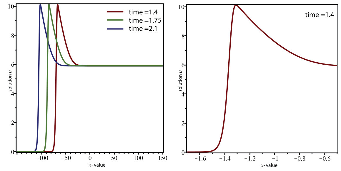 Figure 4
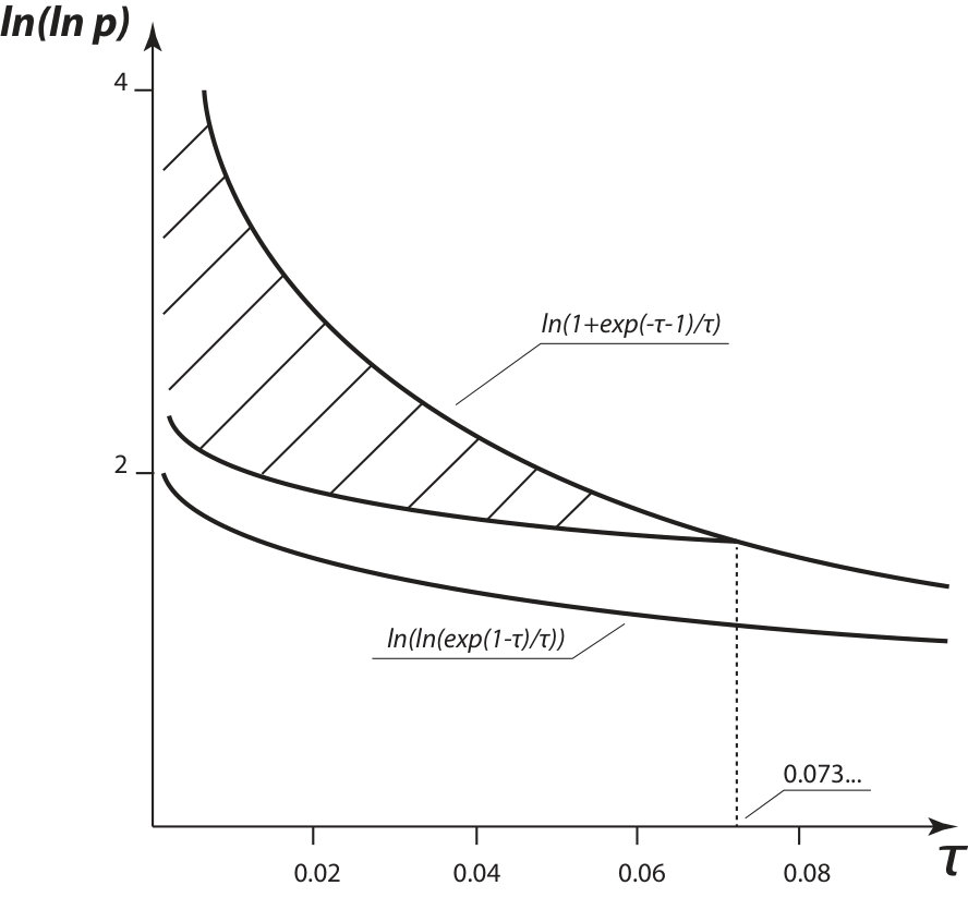 Figure 2
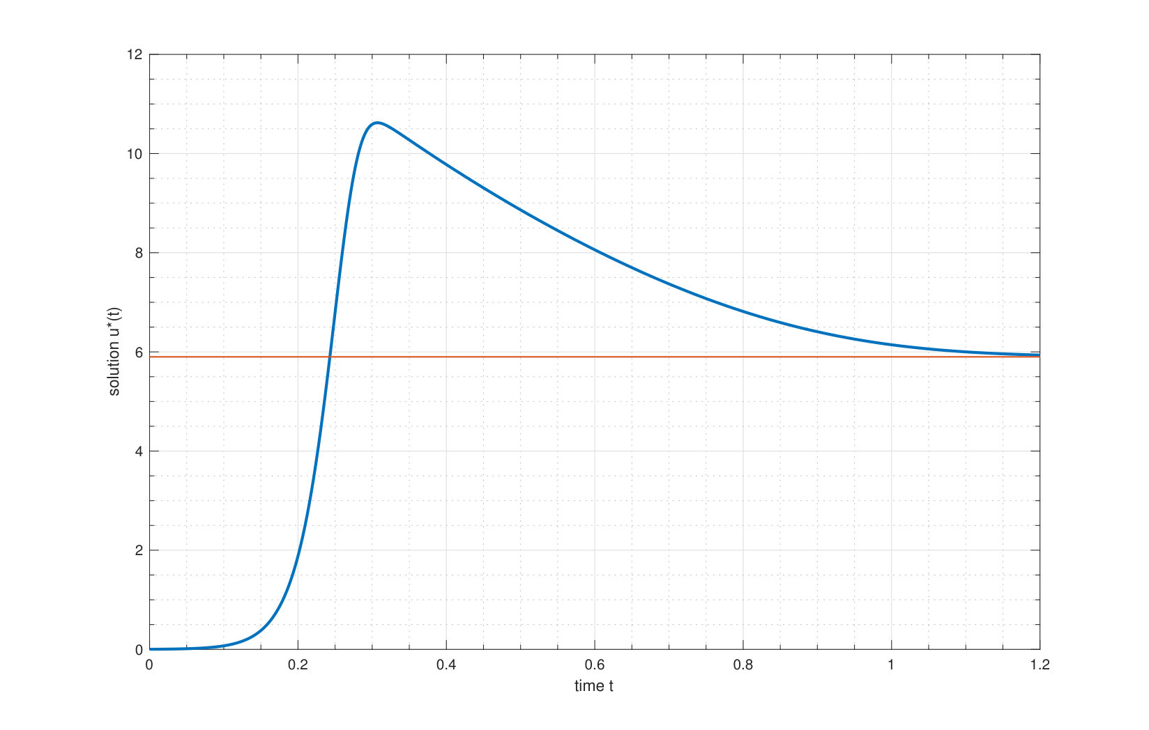 Figure 3
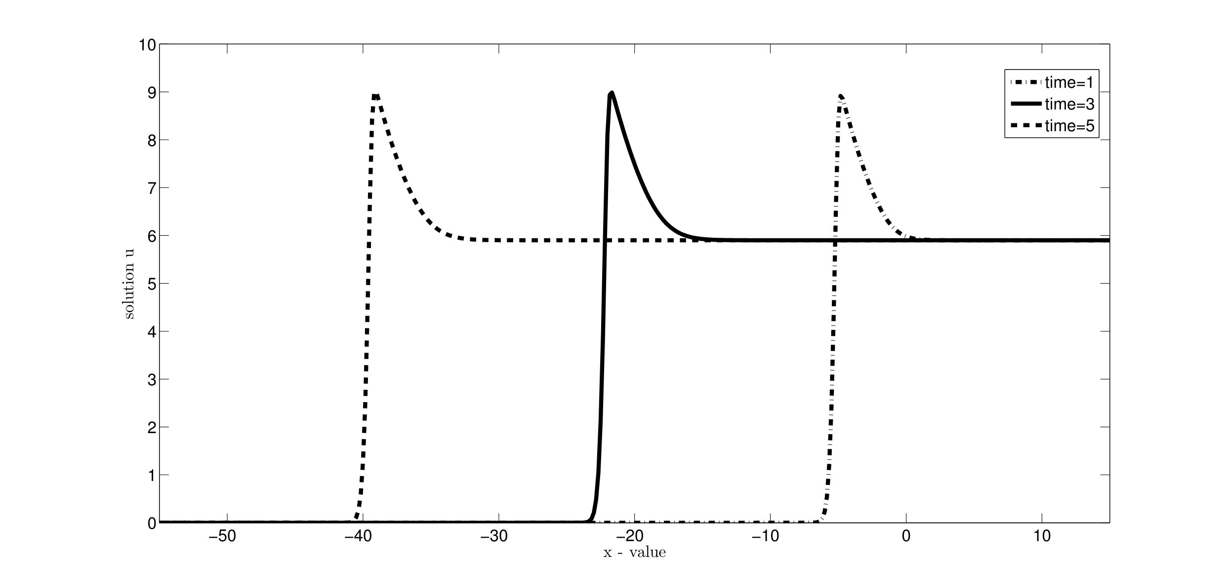 Figure 4
Peer Reviews
No public reviews on file for this paper yet. If you reviewed it on a platform where reviews are public (OpenReview, ICLR, NeurIPS, ICML), you can paste yours below so the community can read it here.
Videos
No videos yet. Explain this paper in a talk, walkthrough, or lecture? Add one.
Nonlinearly determined wavefronts of the Nicholson’s diffusive equation: when small delays are not harmless
Zuzana Chladná
Karel Hasík
Jana Kopfová
Petra Nábělková
Sergei Trofimchuk
Department of Applied Mathematics and Statistics, Faculty of Mathematics, Physics and Informatics, Comenius University, Mlynská dolina, 84248 Bratislava, Slovak Republic
Mathematical Institute, Silesian University, 746 01 Opava, Czech Republic
Instituto de Matemática y Física, Universidad de Talca, Casilla 747, Talca, Chile
Abstract
By proving the existence of non-monotone and non-oscillating wavefronts for the Nicholson’s blowflies diffusive equation (the NDE), we answer an open question from [16]. Surprisingly, these wavefronts can be observed only for sufficiently small delays. Similarly to the pushed fronts, obtained waves are not linearly determined. In contrast, a broader family of eventually monotone wavefronts for the NDE is indeed determined by properties of the spectra of the linearized equations. Our proofs use essentially several specific characteristics of the blowflies birth function (its unimodal form and the negativity of its Schwarz derivative, among others). One of the key auxiliary results of the paper shows that the Mallet-Paret–Cao–Arino theory of super-exponential solutions for scalar equations can be extended for some classes of second order delay differential equations. For the new type of non-monotone waves to the NDE, our numerical simulations also confirm their stability properties established by Mei et al.
keywords:
non-linear determinacy, delay, wavefront, existence, super-exponential solution
2010 Mathematics Subject Classification: 34K12, 35K57, 92D25
††journal: Journal of LaTeX Templates
1 Introduction and main results
Nicholson’s blowflies delay differential equation
[TABLE]
was introduced in 1980 by Gurney, Blythe and Nisbet [21] to provide a better description of the evolution of the population of mature adults of the Australian sheep-blowflies (Lucilia cuprina) observed in a series of highly careful laboratory experiments realized by A. J. Nicholson [33]. The positive parameters are the model’s specific constants and simple scaling of variables allows us to assume that without any restriction of generality. Equation (1) was introduced as a more elaborate alternative to the delayed logistic equation: in difference with (1), the latter was unable to explain some irregular oscillations of observed in the collected experimental data. In a short time, it became clear that Nicholson’s blowflies equation represents a fascinating and non-trivial object of investigation from the dynamical point of view. This fact attracted the interest of numerous researchers over the decades, cf. [4, 15, 29, 33, 35, 45]. Moreover, following the same logic as in the case of the delayed logistic equation (cf. [3]), in 1996 Yang and So [45] introduced the following diffusive version of (1):
[TABLE]
The positive semi-wavefronts , , are the fundamental transitory regimes in the dynamics generated by the diffusive Nicholson’s equation. The existence, uniqueness, oscillation/monotonicity and stability properties of these waves were studied, among many other works, in [7, 12, 15, 16, 26, 27, 37, 38, 39, 44] and the non-local version of (2) was considered, among many other articles, in [17, 18, 19, 20, 24, 25, 28, 36, 46, 47].
In this paper, we revisit the topic of possible shapes for wavefronts , of equation (2). Our first main result, Theorem 1, shows that contrarily to the tacitly accepted hypothesis, cf. [7, 27], of the determinacy of the shape of by the spectra of linearized equations at the equilibria (as it happens, for instance, in the delayed or nonlocal KPP-Fisher equations [8, 11]), equation (2) can have wavefronts which are neither monotone nor oscillating even if the linearization of the profile equation at the positive equilibrium has negative eigenvalues. This implies that a non-monotone wave with unusually high leading edge (see Fig. 1) can appear in (2) even if the associated linearized equations predict the existence of exclusively monotone waves. Surprisingly enough, this strange type of wavefront’s behavior can occur for arbitrarily small delays , to some extent contradicting the folklore principle ”Small delays are harmless” of the theory of delay differential equations [35]. The mechanism behind this loss of monotonicity of wavefronts is precisely the same one which causes the ”linear determinacy principle” [23] to fail for the monostable population models possessing the weak Allee effect (leading to the appearance of pushed or non-linearly determined waves).
In order to state our first result, we introduce some notation. In the sequel, will denote the lower incomplete gamma function, will denote the characteristic function of equation (1) with linearized at :
[TABLE]
It is easy to see that for each equation has exactly one positive root . Set , and
[TABLE]
Theorem 1
Let be such that and . Then there exists such that for each equation (2) has a positive wavefront propagating with the speed and whose profile is eventually monotone at and is non-monotone on . In fact, .
Example 2
Consider ‘small’ delay and take . In such a case, formal linear analysis predicts the existence of a unique monotone wavefront connecting [math] and . However, it is easy to find that , and . Therefore the conclusions of Theorem 1 hold for equation (2) with , . Figure 1 shows a very accurate approximation of the scaled profiles of the corresponding non-monotone and non-oscillating wavefronts (nm-waves, for short) in the limit case . This picture perfectly agrees with the considerations of Remark 17 where we present a numerical solution of (2) with , converging to a wavefront propagating with the large but finite speed .
Theorem 1 and Example 2 answer in positive an open question raised in [16, p. 53] about the existence of an eventually monotone and non-monotone front of (2) for some . In fact, there are many such wavefronts: on Fig. 2, we present the set of parameters satisfying all requirements of Theorem 1. Formally, Theorem 1 works for sufficiently fast wavefronts: since the minimal speed of propagation in Example 2 is relatively large (in the sense that ), one might expect that even the minimal wavefront in Example 2 has non-monotone and non-oscillating profile. Our numerical simulations confirm this informal conclusion: on Fig. 3, we present three consecutive positions (at the times ) of solution for equation (2) with , and with the Heaviside step function as the initial datum. This numerical solution was obtained by applying the second order central difference schemes for the space derivative. The resulting transformed system of ordinary delayed equations has been solved by Matlab built-in function dde23. We take and . This numerical result complements the discussion in Section 7 of [7].
The Nicholson’s blowflies diffusive equation together with the food-limited diffusive equations [22, 40] seem to be the first scalar models coming from applications where untypical behavior in the form of non-monotone non-oscillating wavefronts is established analytically and also observed in numerical experiments. Among previous studies, we would like to mention an illustrative example in [10] of the Mackey-Glass type diffusive equation with a single delay and with a piece-wise linear birth function.
Theorem 1 will be proved in the next section within the framework of the singular perturbation theory developed by Faria et al in [12, 13, 14]. First, in Subsection 2.1, we analyze the unique heteroclinic solution of equation (1). We show that the asymptotic Dirichlet series approximating at is uniformly convergent on a sufficiently long time interval. Then we use these approximations to detect parameters for which is a non-monotone (but eventually monotone at ) and non-oscillating solution of (1). Next, in Subsection 2.2, we extend the aforementioned properties of on the wavefront profiles for all sufficiently large speeds . The key technical result of this subsection is Lemma 15 which excludes the existence of profiles slowly oscillating around the steady state and super-exponentially converging to at . Lemma 15 shows that the Mallet-Paret–Cao–Arino theory of super-exponential solutions [2, 6, 30] for scalar equations can be extended for some classes of second order delay differential equations. Lemma 15 also helps to show that, in difference with the monotone wavefronts, eventually monotone wavefronts are linearly determined:
Theorem 3
Let be a wavefront for equation (2). Then the profile is eventually monotone at if and only if the characteristic function , at the equilibrium has at least one negative zero.
Note that, by [42, Theorem 1], the leading edge of the profile is strictly increasing till its first intersection with the equilibrium level . Eventual monotonicity criterion of Theorem 3 complements previous information concerning the shapes of waves for the Nicholson’s diffusive equation, cf. [16, 27, 42]. It is worth mentioning that our proofs use in an essential way several specific characteristics of the blowflies birth function (in particular, its unimodal form and the negativity of its Schwarz derivative). There are various other monostable population models with unimodal birth functions (e.g., see [3, Table 1], the cases with overcompensating density dependence). We believe that the problem of the nm-waves in these models can be approached by using techniques from the present work. For certain, this does not mean that each population model with overcompensating density dependence [3] necessarily possesses a nm-wave.
Eventual monotonicity criterion of Theorem 3 is proved in Section 2.3 as Corollary 18. We did not succeed to demonstrate this result by using well-known methods of upper and lower solutions or global continuation of waves (these methods were quite efficient in establishing criteria of wave’s monotonicity on [11, 16, 41]). Instead, we have combined the above mentioned Lemma 15 with wavefront’s existence and oscillation results from [42, 43] (stated as Proposition 19 in Appendix). With such an approach, the main technical difficulty was establishing a connection between two different series of conditions (the first one given in Theorem 3 and the second one given in Proposition 19). The required relation (in the form of somewhat cumbersome inequality (22)) is proved in Appendix as Lemma 21.
2 Existence of non-monotone and non-oscillating wavefronts
2.1 On the approximation of the heteroclinic connections for the blowflies equation
In this subsection, we establish several key properties of the positive heteroclinic connections to the Nicholson’s blowflies delayed equation
[TABLE]
The existence and uniqueness of these connections was previously demonstrated in [13, 15], yet the mentioned works did not provide acceptable analytical tools to approximate the unique heteroclinic solution (normalized at ) on a given time interval. Sufficiently sharp approximations are however necessary to prove the existence of the nm-waves, cf. [22]. To obtain such an approximation, we are using here the asymptotic Dirichlet series representing at . It can be deduced from the Murovtsev theory [32] that this series is uniformly converging on some infinite interval . In the next theorem we are trying to find as large as possible by realizing a direct estimation of the Dirichlet series coefficients (in [32], the method of majorization of by analytic functions was used).
Theorem 4
Suppose that and . Then equation (4) has a unique (up to translation) positive solution defined for all satisfying . In addition, is bounded, , and is a real analytic function. Moreover, the solution at can be represented, modulo an appropriate shift in time, by the Dirichlet series
[TABLE]
absolutely and uniformly converging on closed subsets of the interval
[TABLE]
The coefficients , , alternate in sign and can be calculated recursively from equation (4). In particular, , with defined in (3).
Proof 1
We look for an analytic solution of equation (4) in the form
[TABLE]
with some . After comparing the coefficients of in both sides of the next equation (obtained from (4) by using a series representation for )
[TABLE]
we get the recurrent formula determining , :
[TABLE]
The general term of the sum in brackets is
[TABLE]
Assuming that for all , we find that is
[TABLE]
Therefore . Notice here that for all .
Suppose now that for each . Then, invoking elementary combinatorics together with the Egorychev method [9], we find that, for each ,
[TABLE]
[TABLE]
[TABLE]
[TABLE]
[TABLE]
whenever and . Thus, for each , the Dirichlet series (6) with converges absolutely and uniformly on each closed subset of . Equivalently, the shifted series
[TABLE]
converges for all . Hence, equation (4) has an analytic solution defined and positive on some interval . Clearly, integrating (4) step by step, we can extend this solution for all . Next, the set is invariant with respect to the semi-flow generated by (4) so that for all . Furthermore, since all solutions to (4) are uniformly persistent when [4, Theorem 2.4], the trajectory , where , has a compact -limit set in . In particular, is bounded and . Then by the classical Nussbaum theorem [34], is a real analytic function on . Finally, the uniqueness of was established in the proofs of [13, Lemmas 6 and 8]. Alternatively, it can be deduced from the general uniqueness Theorem 3 in [1]. \qed
Remark 5
Suppose that either or and
[TABLE]
Then [29, Theorem 2.1] implies that the positive solution given in Theorem 4 converges at : .
Example 6
As in Example 2, take and and choose . Then Theorem 4 provides the convergence interval for the series (5). In addition, in this particular case, are decreasing which suggests the following estimates for in the spirit of the alternating series test:
[TABLE]
Our next result shows that this estimate is indeed true.
Theorem 7
Solution described in Theorem 4 and normalized at by (5) satisfies (8).
Proof 2
In view of Theorem 4, the inequalities (8) hold on some interval with . It is easy to see that for all . Indeed, suppose that at some leftmost point . Then , , so that
[TABLE]
[TABLE]
a contradiction. Hence for all . In particular, for all .
Next, we have that
[TABLE]
Since if and only if , we conclude that whenever .
We claim that actually the first inequality in (8) also holds for all . Since for all , it suffices to prove it only for those for which . Arguing by contradiction again, suppose that at some leftmost point . Then , so that
[TABLE]
a contradiction. Observe here that the strict monotonicity of on the interval plays an essential role in the last argument. \qed
We will also need the following property of :
Lemma 8
* on some maximal interval . Clearly, if , then . If is finite, then .*
Proof 3
By differentiating (5), we find that at , from which the existence of the above mentioned follows. Suppose that is finite, then . Since (4) implies the relation , we obtain so that . Clearly, if also then and the lemma is proved in such a case. On the other hand, if then the statement follows from the relation . \qed
Now, looking for wavefronts to (2) in the form
[TABLE]
we obtain the profile equation
[TABLE]
Equation (9) was analyzed in [1, 13, 15, 16, 26, 27, 37, 42]. Since the first derivative of is dominated by , for all , the uniqueness (up to translation) of each semi-wavefront to (9) follows from [1, Theorem 7]. Next, by [37] or [42, Corollary 12] if (i.e. if is monotone on ) then for all . Now, when , is no longer monotone on . Nevertheless, in such a case for all and satisfies the feedback condition on the interval (see condition (18) in Appendix). Therefore [16, 42] assure that if then is either monotone or sine-like slowly oscillating around at ; moreover, the type of monotonicity/oscillation property is linearly determined. Similarly, [16, Theorem 2.5] implies that is strictly increasing when and . Next, it is easy to see that the characteristic equation does not have real negative roots when . Then [42, Lemma 25] implies that cannot be eventually monotone if . Hence, we have established the following result:
Lemma 9
Suppose that equation (2) has a nm-wave. Then necessarily , and . In particular, where solves equation .
Corollary 10
If equation (2) has a nm-wave then and .
Proof 4
Indeed, . Set , then implying that . Consequently, and , \qed
In the next stage of our proof, we continue to analyze the heteroclinic solution given in Theorem 4. This time, we will take parameters as in Lemma 9 which will have important consequences for the form and estimates of . For example, in such a case, due to Corollary 10 the lower bound in (8) is positive for all . Especially we will be interested in the oscillation properties (around the equilibrium ) of . Since is a real analytic function on , the set of all solutions of equation is either an empty set or can be represented as a strictly increasing sequence of positive numbers. By the same reason, if the sequence is infinite, it should converge to . Our next goal is to prove that are simple zeros of and that . The main complication here consists in the fact that the birth function for does not satisfy the feedback condition (18), cf. [16, 42]. Our arguments below are inspired by the classical theory of J. Mallet-Paret [30].
Lemma 11
Suppose that and . Then inequality (7) is satisfied so that and, in fact, is eventually monotone solution. Furthermore, the above defined sequence has at most a finite number of elements, , and , for each such .
Proof 5
It is easy to check that the smooth curves defined by equations and , respectively, intersect at some point if and only if satisfies equation . However, a straightforward comparison of the Taylor coefficients in this equation shows that for all positive . Hence, . Actually, an easy inspection shows that the domain bounded by and the coordinate axes lies inside the domain bounded by and the coordinate axes.
Now, suppose that is the moment of the first intersection of the graph of with the line . Then in view of Lemma 8. Suppose next that is the moment of the second intersection of with the line and . Then , from which we obtain , . In the case when we have, in addition, that . Consider first the situation when . Then implies that . On the other hand implies that . Thus , a contradiction. Finally, suppose that . Then implying the following contradictory relation . The above discussion shows that and that .
By our convention, for and for some leftmost . Again, . Since , the latter implies that and, consequently, that . Therefore, using the variation of constant formula, we get
[TABLE]
In particular, for all . Now, since , we find that . This implies that . Suppose that , then obviously (since are the consecutive zeros of ) and , a contradiction. Consequently, , and .
Next, for and . Thus from where (here we are using the inequality for ). Suppose that , then again we get and , a contradiction. Consequently, , and . Clearly, the above described inductive steps can be continued to include all points .
Finally, we will prove that the sequence is finite. Linearizing (1) at the equilibrium , we find the associated characteristic function After a straightforward computation, we find that has exactly two different real roots if and only if . Moreover, in such a case, each other root , satisfies the inequalities and , see [30, Theorem 6.1]. In particular, the steady state is exponentially stable. We claim that is eventually monotone at if . Indeed, otherwise, it is easy to see that the sequence is infinite so that exponentially converges to the equilibrium and slowly oscillates around it. Then in view of Yulin Cao results [6, Theorem 3.4] on super-exponential solutions, there is a zero of and such that
[TABLE]
Now, if is not a real root, the above representation implies that the distance between large adjacent zeros of is less than , a contradiction. Hence
[TABLE]
where . This completes the proof of Lemma 11. \qed
Importantly, the sequence can be non-empty for certain parameters . The next result shows that generally in Lemma 11. It is an open question, however, whether there exist for which .
Corollary 12
In addition to the assumptions of Lemma 11, suppose that where was defined in Theorem 1. Then the solution is eventually monotone at and is non-monotone on . Moreover, .
Proof 6
Indeed, after using the variation of constant formula on and monotonicity of on the interval , we find that
[TABLE]
[TABLE]
[TABLE]
Finally, recall that for the parameters , see Example 2. \qed
2.2 Proof of Theorem 1
The key relation between and is given in the next assertion.
Proposition 13
Let all the conditions of Corollary 12 be satisfied. Then for all sufficiently small . Moreover, uniformly on (possibly, after an appropriate translation of the wavefronts). In particular, the wave profiles are not monotone for all small .
Proof 7
First, suppose that the characteristic equation does not have roots on the imaginary axis. Then, in view of the uniqueness of semi-wavefronts in the Nicholson’s blowflies diffusive equation, the statement concerning the uniform convergence is a direct consequence of [13, Theorem 1]. Now, if the zero equilibrium of equation (1) is not hyperbolic, the same conclusion follows from Theorem 3.8 in [14]. \qed
To complete the proof of Theorem 1, we have to extend the eventual monotonicity property of established in Lemma 11 on the profiles for all sufficiently small . Observe that, taking into account Proposition 13 and using [31, Theorem 2.1] we obtain (see [42, pp. 2321-2322] for more detail) that is either eventually monotone or slowly oscillating around at in the following sense:
Definition 14
Set . For any we define the number of sign changes by
[TABLE]
We set if or for . Next, for a smooth function and a real number , we will write if , and . We will say that is slowly oscillating around on a connected interval if the following conditions are satisfied:
(d1) oscillates around and
(d2) for each , it holds that either sc or sc.
Therefore our immediate goal is to demonstrate that is not a slowly oscillating solution of equation (9) whenever all the conditions of Corollary 12 are satisfied. We have already solved a similar problem, proving eventual monotonicity of in Lemma 11. However, trying to argue as at the end of the proof of Lemma 11, we will regret the lack of an analog of the Mallet-Paret–Cao–Arino theory [2, 6, 30] of super-exponential solutions (i.e. solutions converging to their finite limits at faster than any exponential) for the second order delay differential equations. The key idea of this theory was concisely described by Ovide Arino: ”Surprisingly, the proof is based on quite an elementary although very neat observation, which is, essentially, if you assume a solution has a rapid decay from to , it indicates rapid oscillations before ”, see [2, p. 178]. In our next lemma, we contribute to the analysis of super-exponential solutions by developing this idea for second order delay differential equations (at a level of generality sufficient for our purposes).
Lemma 15
Let slowly oscillate around [math] and satisfy equation
[TABLE]
where and continuous function converges to a positive number at . Suppose also that the set of zeros of does not contain a non-degenerate interval. Then is not a super-exponentially decaying (i.e. small) solution.
Proof 8
Arguing by contradiction, suppose that equation (11) has a slowly oscillating small solution . After realizing the change of variables , where is a negative root of equation , we obtain the delay differential equation for of the same type as (11) (i.e. , ) except that now :
[TABLE]
Obviously, is super-exponentially decaying at . It is easy to check that, being a small solution, with shares the slow oscillation property of . We will arrive to a contradiction by supposing the existence of a slowly oscillating small solution of equation (12).
Hence, arguing by contradiction, suppose that equation (12) has a slowly oscillating small solution . In our subsequent argumentation, we will use the notation so that and . It is easy to see that the ‘smallness’ of implies the existence of an increasing sequence , , such that as (since oscillates, we have that for each ).
Set , clearly for and for some . Without loss of generality, we can further assume that and that for some . Due to our choice of , we also find that uniformly on the interval . In addition, is a slowly oscillating small solution of the differential equation
[TABLE]
We will say that an interval is a maximal complete interval of monotonicity for some if is monotone on , and is not properly contained in a larger interval with the same properties. Then there exists some such that and . Thus
[TABLE]
so that can have at most 3 maximal complete intervals of monotonicity on each interval of length (consequently, at most 5 intervals of monotonicity). As a consequence, we can find a subsequence of such that that all have exactly the same number of intervals of monotonicity inside of each of the segments , while the sequences are converging to their respective limits . Without loss of generality, we can also assume that every does not change its sign on each of the intervals . Furthermore, due tho the Helly selection theorem [5, p. 250], we can assume that there exists a piece-wise monotone function such that and pointwise on . In the sequel, to simplify the notation, we will denote by also any subsequence of .
We claim that almost everywhere on . First, observe that the sequence of the total variations of the smooth functions on converges to 0. Then, by the Riesz theorem [5, p. 79], we can extract a subsequence such that almost everywhere on . Take some , , such that . By integrating (13), we find that
[TABLE]
Passing to the limit in (14), we find that, for almost all ,
[TABLE]
which proves our claim.
Now, fix some non-empty monotonicity interval mentioned before. Due to the claim of the previous paragraph, we know that there are such that . Then we find immediately that and uniformly on . Arguing now as in the previous paragraph and passing to subsequences if necessary, we can conclude that almost everywhere on . Hence, we have proved that there exists a finite set of points such that uniformly on each closed interval . Consequently, almost everywhere on and .
In the next stage, we will analyze the sequence on the interval . Set and consider some closed interval . For all sufficiently large , the functions have the same type of positivity and monotonicity on . We claim that we can choose a subsequence in such a way that uniformly on . To be more specific, suppose, for example, that are non-negative and decreasing on . If some subsequence of converges to for , then clearly uniformly on while almost everywhere on . But then, after taking some , , such that and using (14), we immediately get a contradiction. This implies that the sequence is bounded for each . In fact, since we can slightly move the endpoints of this interval, the sequences are also bounded. This allows us to conclude that is uniformly bounded on . Consequently, by arguing as above and passing to subsequences if necessary, we find that uniformly on and almost everywhere on . In other words, have similar convergence properties on the intervals and .
Therefore, in each -neighborhood of , we can find points such that , (whenever is sufficiently large) and , , . Similarly, the interval contains a point such that .
But then, if , there are some points satisfying the inequalities and the relations , . Since , we can also assume that . Consequently, in view of equation (13),
[TABLE]
[TABLE]
Now, since , for each big enough we can find points such that , , . Thus Finally, consider four points . Since , we conclude that sc so that does not slowly oscillate around [math]. The obtained contradiction completes the proof of Lemma 15. \qed
Corollary 16
Assume all the conditions of Corollary 12. Then there exists such that the solution is eventually monotone at for each
Proof 9
After linearizing (9) at the equilibrium , we find the related characteristic equation
[TABLE]
If , it follows from [16, Lemma 1.1] and [43, Lemma 2.1] that there are and such that (15) has in the half-plane for each exactly three roots . Moreover, these roots are real and , and as (as in Lemma 11, here denote the zeros of ). Therefore the steady state of (9) is hyperbolic and the orbit associated with belongs to the stable manifold of . Thus and have at least the exponential rate of decay at . Now, arguing by contradiction, suppose that the function oscillates slowly around [math]. Clearly, satisfies equation (11) where , . But then Lemma 15 guarantees that has at most the exponential rate of decay at . This implies that there is a complex zero , of and such that
[TABLE]
Now, by Lemma 21 in [42], and therefore does not oscillate slowly around [math]. The obtained contradiction completes the proof of Corollary 16. \qed
Clearly, Theorem 1 is a direct consequence of Proposition 13 and Corollaries 12 and 16.
Remark 17
On Fig. 4, we present a fast traveling wave for equation (2) with , . The numerical simulations are based on the Crank-Nicholson method which is second-order accurate in both spatial and temporal directions. The initial function is
[TABLE]
The spatial step size is chosen as in the computational domain where the Dirichlet boundary conditions and are imposed. The temporal step size is . After some short initial period, the numerical solution behaves like a nm-wave moving leftward with the speed . This provides an additional numerical confirmation of the theoretical result in [27] in the case of nm-waves (theoretical speed of propagation is ). Observe that the rescaled profile is rather well approximates the limit profile, , on the Fig.1.
2.3 Proof of Theorem 3
Theorem 3 follows from the following equivalent statement:
Corollary 18
Let be a wavefront for equation (2). Then the profile is eventually monotone at if and only if the characteristic function with has at least one negative zero.
Proof 10
Suppose that equation (2) has an eventually monotone wavefront . Then it follows from the proof of Lemma 25 in [42] that has a negative zero.
Conversely, suppose that, given a fixed pair of positive parameters, equation (2) possesses a semi-wavefront and has a negative zero . We will denote the latter fact as , where
[TABLE]
We have to prove that, in such a case, is monotone in some neighborhood of . First, consider . Then is necessarily monotone on in view of So and Zou main theorem in [37] and the semi-wavefront uniqueness [1, 39, 44]. Second, if , then the monotonicity of on was established in [16, Theorem 2.3].
Hence, in what follows, we can assume that . Then the relation (21) in the appendix says that . In consequence, since , Proposition 19 guarantees that (i.e. is a wavefront). Moreover, decays exponentially to [math] as (e.g. see [16, Lemma 1.1] or [43, Proposition 5.6]).
Arguing by contradiction, suppose now that oscillates around on some connected neighborhood of . We claim that these oscillations are necessarily slow on .
Indeed, if satisfies the feedback condition (18) and (equivalently, or , cf. [16, Corollary 2.4]), then the slow oscillation property of follows from Proposition 19.
Suppose now that and consider the oscillating wavefront of equation (9). By Proposition 19, the first three critical points of are finite and such that on on and . We will prove that for all . First, we observe that, by [43, Lemma 4.2]
[TABLE]
where denote the roots of the equation , is the unique point in where and . Since , , and for , we immediately find that
[TABLE]
Thus for all and if at some point , then there exists the leftmost critical point such that and . In particular, . Since, in addition, equation (9) implies that , we obtain that . Therefore for some . Invoking again formula (16), we find that . This contradiction proves that actually for all . Therefore the feedback condition (18) is satisfied on the set . Since the slow oscillation property of follows now from Proposition 19 and Corollary 14 in [42], the claim is proved.
Finally, arguing as in the second half of the proof of Corollary 16, we conclude that the assumption is not compatible with the existence of slowly oscillating (around ) and exponentially converging (toward ) wavefront . Therefore is monotone at . \qed
3 Appendix
In this section, we are use the notation
[TABLE]
The next assertion follows from [43, Theorem 1.1] and [42, Theorems 3, 13], is instrumental in proving Theorem 3 (or Corollary 18) of this paper and is given for the convenience of the reader. We consider the following restrictions on the nonlinearity :
(H)
Let have only one critical point (maximum) and assume that and . Suppose further that that the equation has exactly two roots with , and that the Schwarz derivative is negative for all :
[TABLE]
Proposition 19
Assume (H), suppose that the equation has at least one positive root, and
[TABLE]
Then equation (9) has a positive wavefront . Furthermore, if is non-monotone on , then there exist , such that on and on . If is finite then and . Finally, if satisfies the feedback condition
[TABLE]
*then is either eventually monotone or oscillates slowly (see Definition 14) around . *
Lemma 20
For each fixed and , equation
[TABLE]
has a unique positive root . The function is smooth and has a finite limit .
Proof 11
It is easy to check that for all . Taking into account that , and , we deduce the existence of the unique solution of equation (19). Now, let be the limit of sequence with . Then necessarily which proves the uniqueness and finiteness of . Thus \qed
In the first quadrant of the plane , given a fixed number , together with the above defined set of parameters , we consider also the following domain
[TABLE]
Lemma 20 shows that . On the other hand, it was established in [16, Section 2.3] that , where is defined as the unique positive solution of equation
[TABLE]
By [16, Lemma 1.1], is a smooth decreasing function such that , , where . Observe that for so that . In fact, the next lemma assures that for all so that
[TABLE]
Lemma 21
For each and , it holds that
[TABLE]
Proof 12
With , inequality (22) is equivalent to
[TABLE]
For fixed , we equation maximize and minimize with respect to . The second task is easy: . To maximize , we will introduce the new variable , . Then takes the form
[TABLE]
We will further simplify :
[TABLE]
We claim that, for all , . First, we rewrite this last inequality in the following equivalents forms:
[TABLE]
[TABLE]
[TABLE]
[TABLE]
[TABLE]
[TABLE]
to be proved for all It is convenient to represent in the form of the power series:
[TABLE]
[TABLE]
where ,
[TABLE]
[TABLE]
[TABLE]
It follows from the above expressions that for all and since for all , it holds that
[TABLE]
as well as for
[TABLE]
[TABLE]
we conclude that for all , and for all . This proves that for all , and for all . Hence, to complete the proof of the positivity of for all and , it suffices to establish that for all . Now, or, equivalently, will be positive for all and for some fixed if the discriminant
[TABLE]
[TABLE]
will be negative for this value of . Observe that is the product of two quadratic polynomials so that it is immediate to see that for all . In a consequence, for all and and also .
Finally, the positivity of assures that . \qed
Acknowledgments
The work of Karel Hasík, Jana Kopfová and Petra Nábělková was supported by the institutional support for the development of research organizations IČO 47813059. This work was realized during a stay of Sergei Trofimchuk at the Silesian University in Opava, Czech Republic. This stay was possible due to the support of the Silesian University in Opava and the European Union through the project CZ.02.2.69/0.0/0.0/16_027/0008521. S. Trofimchuk was also partially supported by FONDECYT (Chile), project 1190712.
The reference list from the paper itself. Each links out to its DOI / PubMed record.
- 1[1] M. Aguerrea, C. Gomez, S. Trofimchuk, On uniqueness of semi-wavefronts (Diekmann-Kaper theory of a nonlinear convolution equation re-visited), Math. Ann. 354 (2012) 73-109.
- 2[2] O. Arino, A note on “The discrete Lyapunov function…,” J. Differential Equations 104 (1993), 169–181.
- 3[3] M. Bani-Yaghoub, G.-M. Yao, M. Fujiwara, D.E. Amundsen, Understanding the interplay between density dependent birth function and maturation time delay using a reaction-diffusion population model, Ecological Complexity 21 (2015) 14–26.
- 4[4] L. Berezansky, E. Braverman, L. Idels, Nicholson’s blowflies differential equations revisited: Main results and open problems, Appl. Math. Modelling 34 (2010) 1405–1417.
- 5[5] Y. M. Berezansky, Z. G. Sheftel, G. F. Us, Functional Analysis, Vol. I-Birkhäuser Basel, 1996.
- 6[6] Y. Cao, The discrete Lyapunov function for scalar differential delay equations, J. Differential Equations 87 (1990), 365–390.
- 7[7] I.-L. Chern, M. Mei, X.-F. Yang, Q.-F. Zhang, Stability of non-monotone critical traveling waves for reaction-diffusion equations with time-delay, J. Differential Equations 259 (2015) 1503–1541.
- 8[8] A. Ducrot, G. Nadin, Asymptotic behaviour of traveling waves for the delayed Fisher-KPP equation, J. Differential Equations 256 (2014) 3115–3140.