Warm Absorber Diagnostics of AGN Dynamics
T. Kallman, A. Dorodnitsyn

TL;DR
This paper uses dynamical models to generate synthetic spectra of warm absorbers in AGN, aiming to understand their physical mechanisms, distribution, and relation to ultrafast outflows by comparing with observations.
Contribution
It introduces ab initio dynamical models to simulate warm absorber spectra, providing a new observational test for different physical scenarios in AGN outflows.
Findings
Observed spectra constrain the geometry of warm absorbers.
Not all dynamical models reproduce observed spectral features.
Some scenarios are more successful in matching observations.
Abstract
Warm absorbers and related phenomena are one of the observable manifestations of outflows or winds from active galactic nuclei (AGN). Warm absorbers are common in low luminosity AGN, they have been extensively studied observationally, and are well described by simple phenomenological models. However, major open questions remain: What is the driving mechanism? What is the density and geometrical distribution? How much associated fully ionized gas is there? What is the relation to the quasi-relativistic 'ultrafast outflows' (UFOs)? In this paper we present synthetic spectra for the observable properties of warm absorber flows and associated quantities. We use ab initio dynamical models, i.e. solutions of the equations of motion for gas in finite difference form. The models employ various plausible assumptions for the origin of the warm absorber gas and the physical mechanisms affecting…
Click any figure to enlarge with its caption.
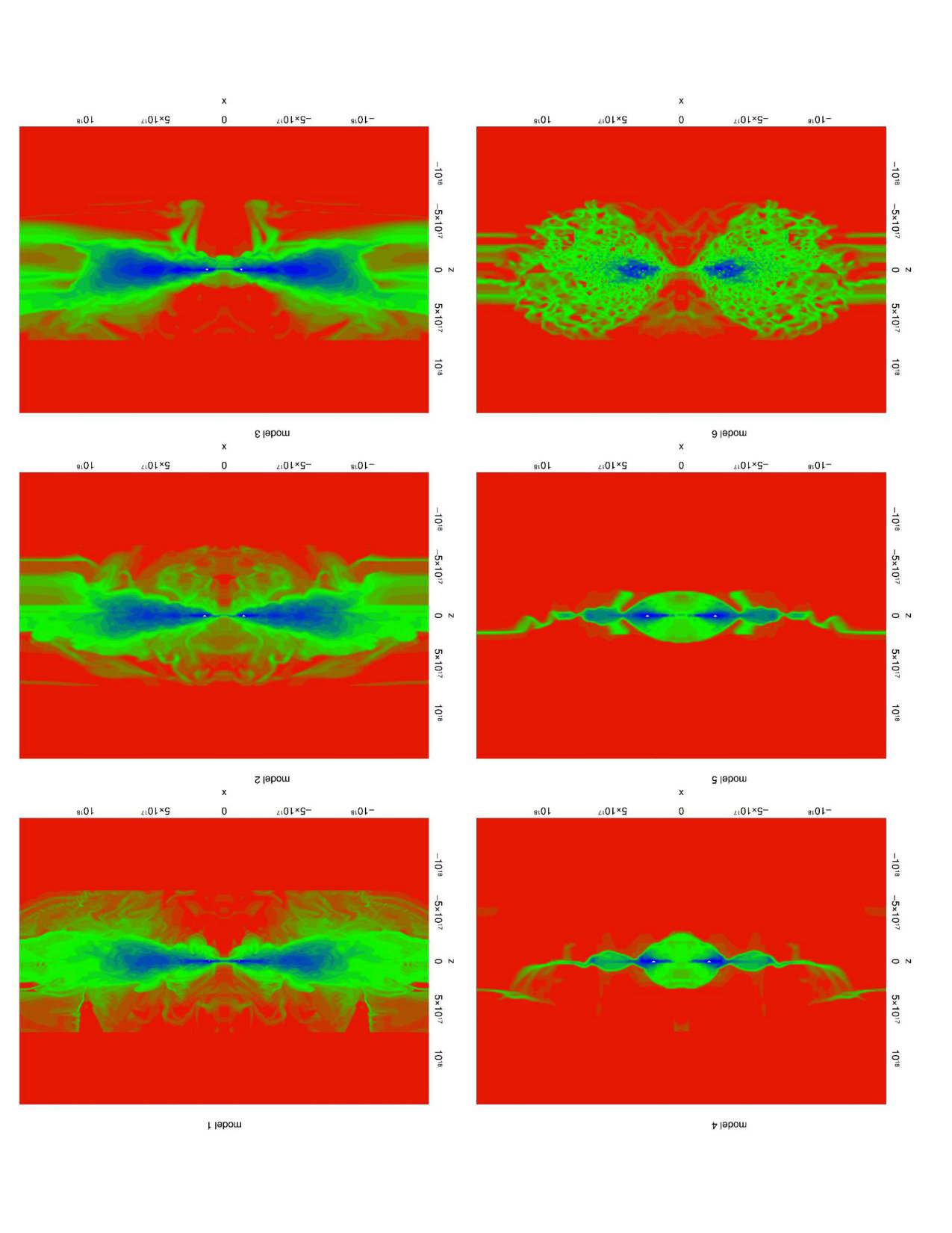 Figure 1
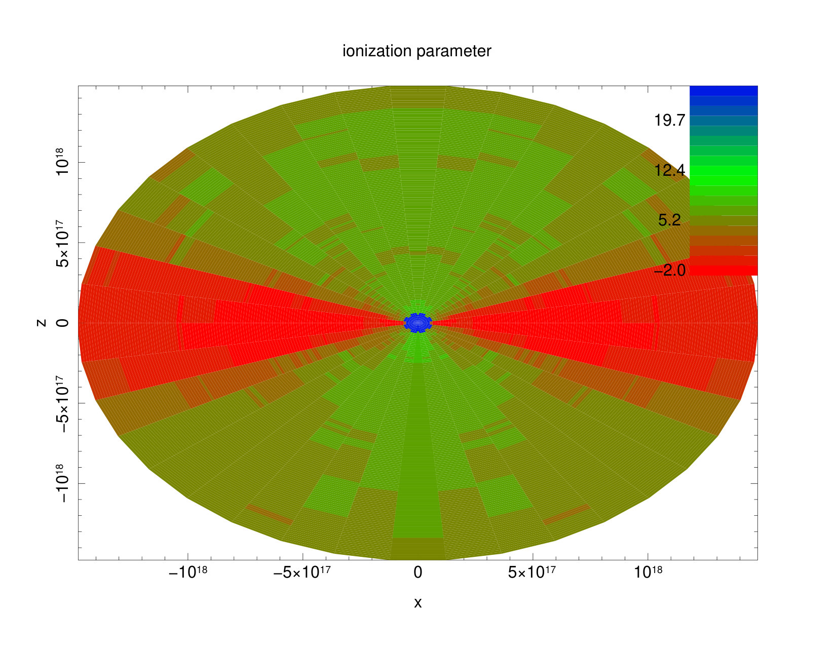 Figure 2
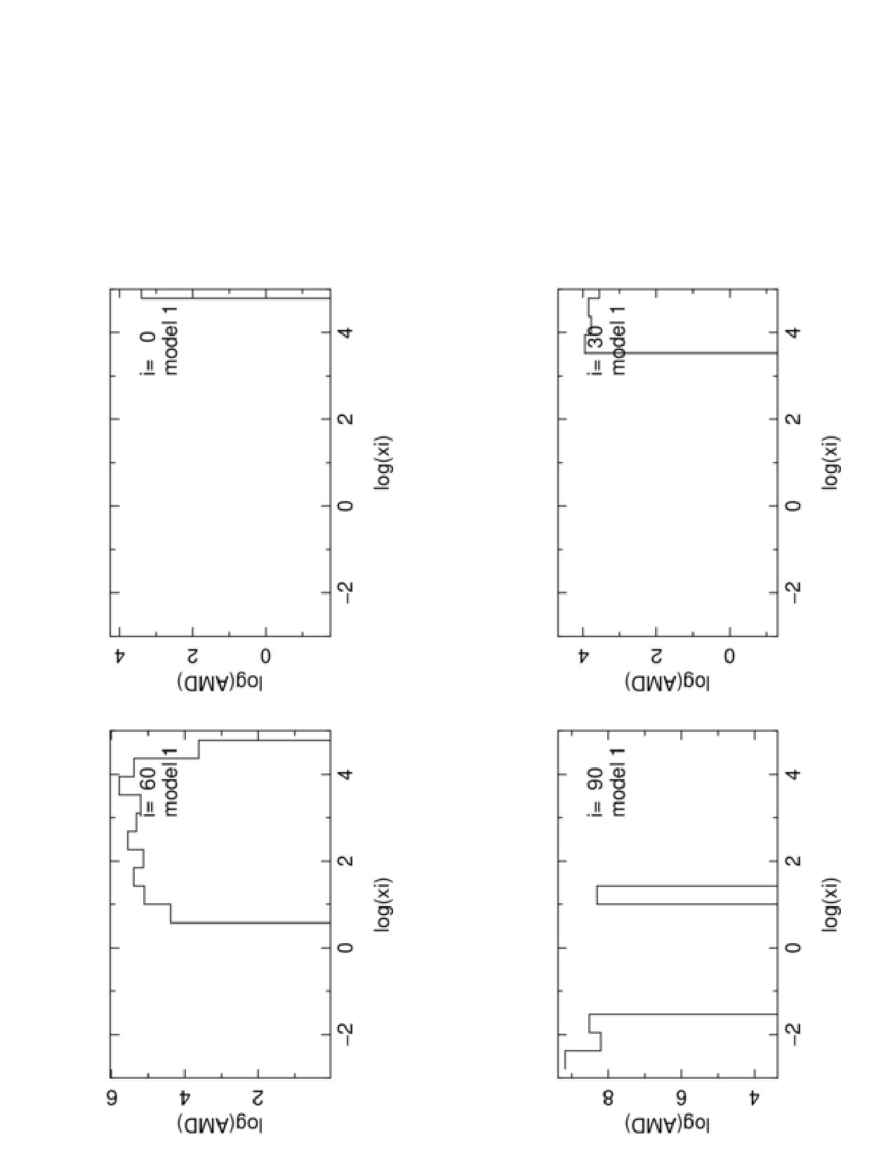 Figure 3
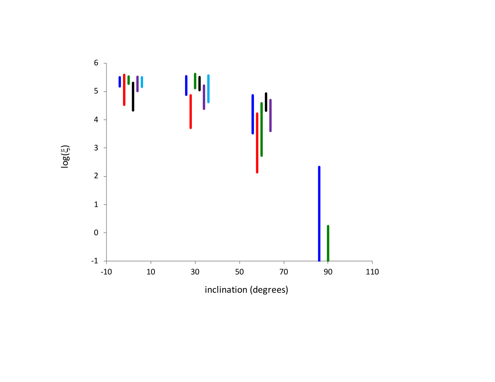 Figure 4
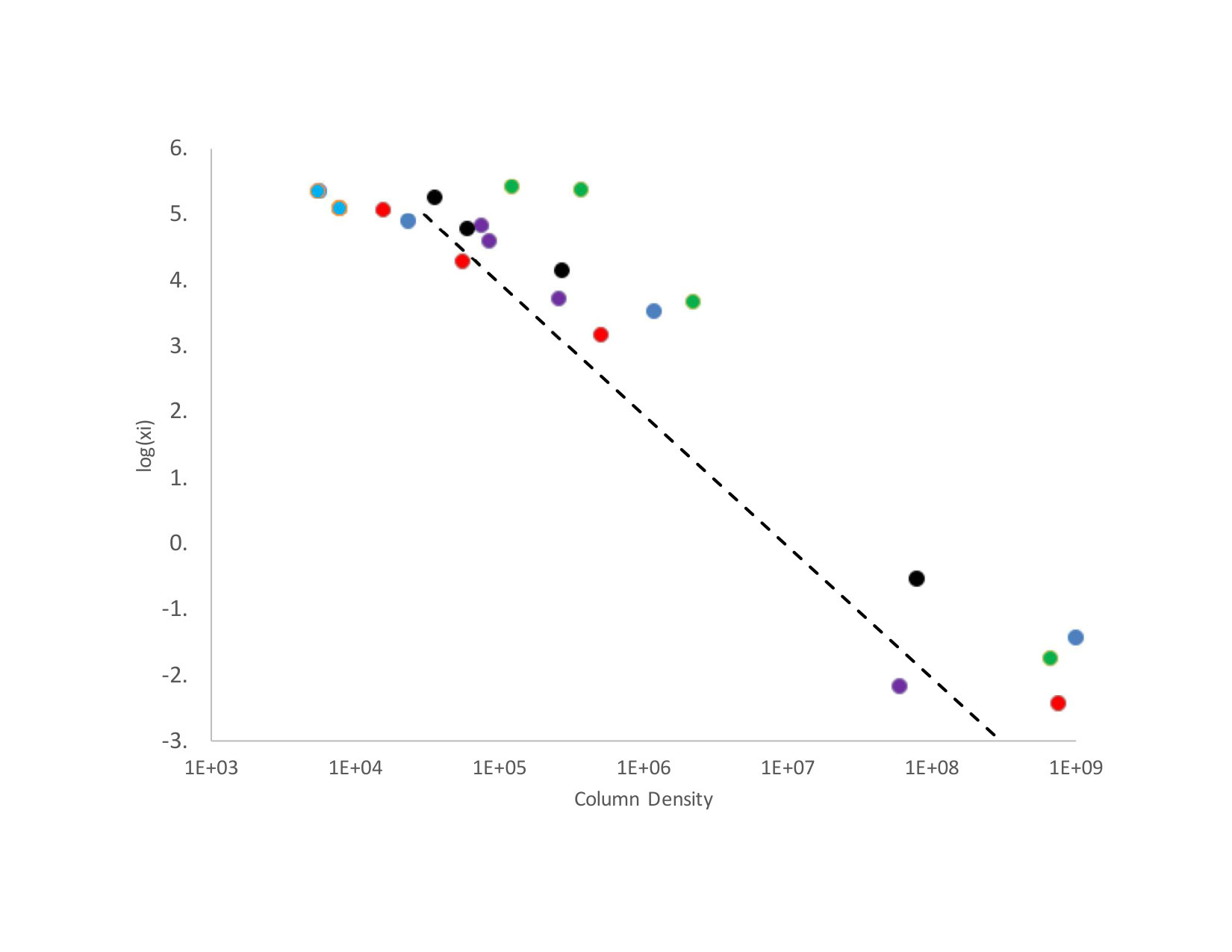 Figure 5
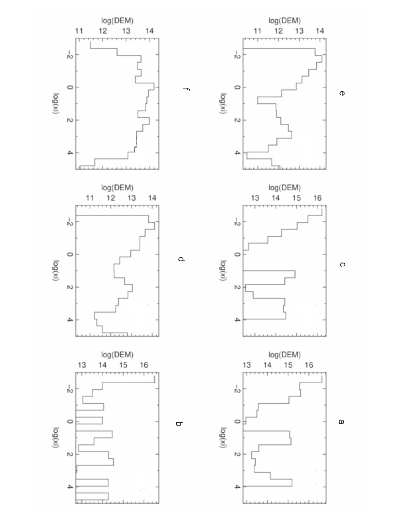 Figure 6
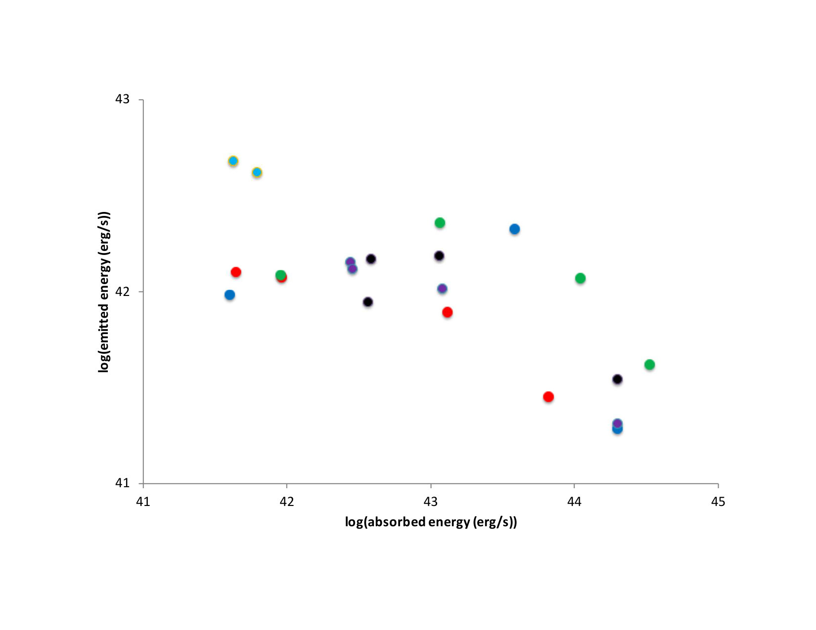 Figure 7
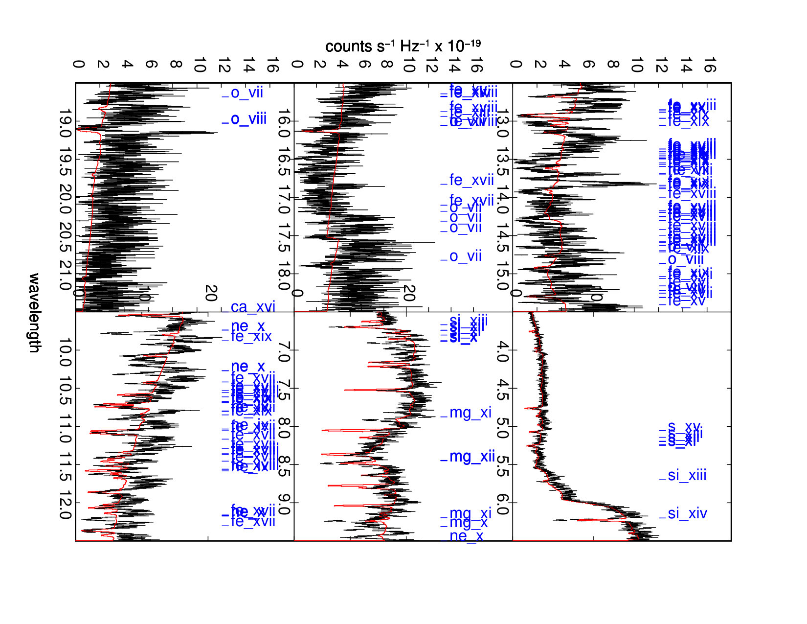 Figure 8
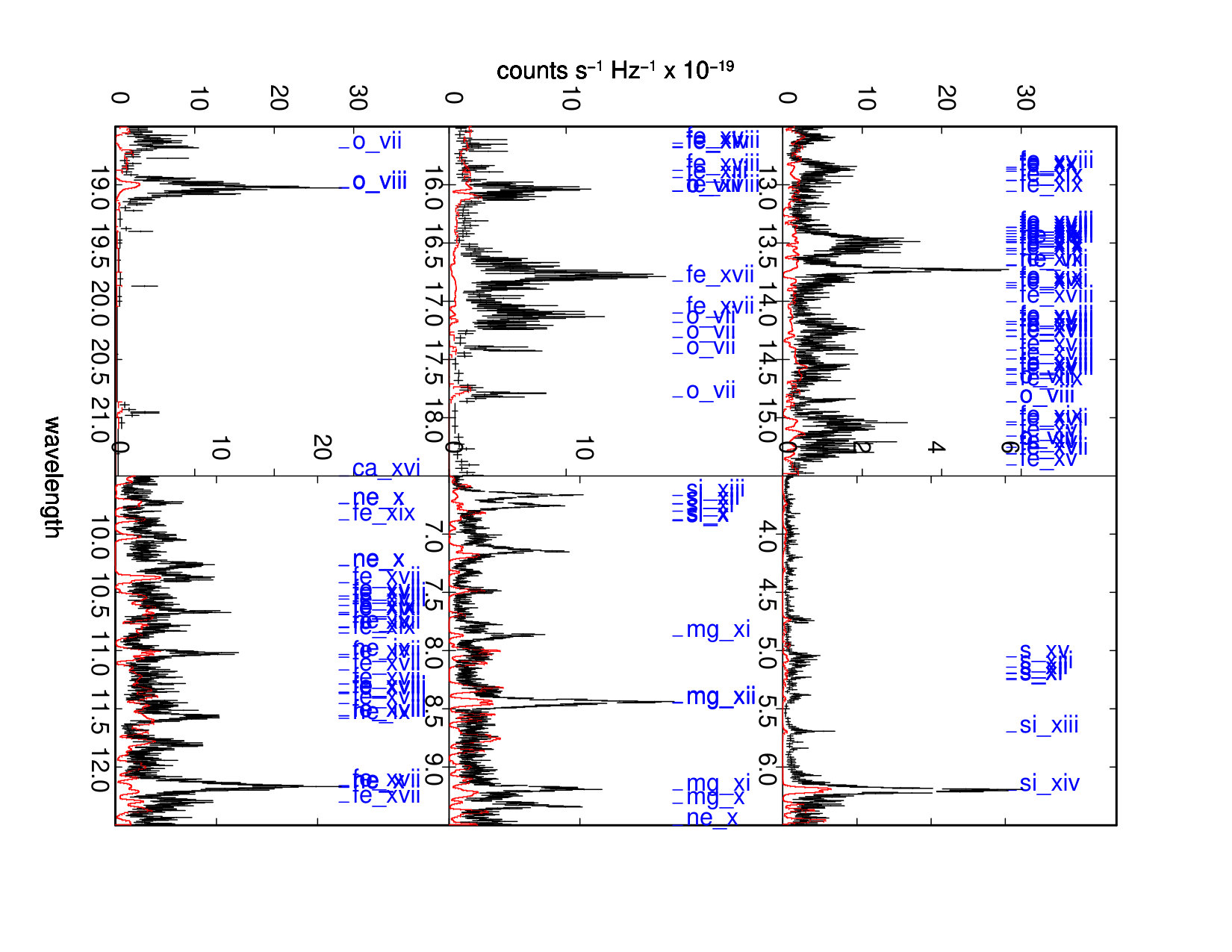 Figure 9
| Model | L (erg s-1) | MTorus (gm) | note |
|---|---|---|---|
| 1 | 3E+45 | 1.45E+38 | TOR |
| 2 | 1E+45 | 1.44E+38 | TOR |
| 3 | 5E+45 | 1.45E+38 | TOR |
| 4 | 1E+45 | 9.15E+36 | SOL |
| 5 | 3E+45 | 8.90E+36 | SOL |
| 6 | 3E+45 | 1.06E+37 | hydro |
Peer Reviews
No public reviews on file for this paper yet. If you reviewed it on a platform where reviews are public (OpenReview, ICLR, NeurIPS, ICML), you can paste yours below so the community can read it here.
Videos
No videos yet. Explain this paper in a talk, walkthrough, or lecture? Add one.
Taxonomy
TopicsGalaxies: Formation, Evolution, Phenomena · Stellar, planetary, and galactic studies · Gamma-ray bursts and supernovae
Warm Absorber Diagnostics of AGN Dynamics
T. Kallman, A. Dorodnitsyn 11affiliation: NASA/GSFC, Code 662, Greenbelt MD 20771
Abstract
Warm absorbers and related phenomena are one of the observable manifestations of outflows or winds from active galactic nuclei (AGN). Warm absorbers are common in low luminosity AGN, they have been extensively studied observationally, and are well described by simple phenomenological models. However, major open questions remain: What is the driving mechanism? What is the density and geometrical distribution? How much associated fully ionized gas is there? What is the relation to the quasi-relativistic ’ultrafast outflows’ (UFOs)? In this paper we present synthetic spectra for the observable properties of warm absorber flows and associated quantities. We use ab initio dynamical models, i.e. solutions of the equations of motion for gas in finite difference form. The models employ various plausible assumptions for the origin of the warm absorber gas and the physical mechanisms affecting its motion. The synthetic spectra are presented as an observational test of these models. In this way we explore various scenarios for warm absorber dynamics. We show that observed spectra place certain requirements on the geometrical distribution of the warm absorber gas, and that not all dynamical scenarios are equally successful at producing spectra similar to what is observed.
1. Introduction
Warm absorber spectra in the X-ray band consist of absorption features from gas with a range of ionization states, from near-neutral to hydrogenic for medium-Z elements, with line widths and blueshifts 1000 km s*-1*. They are seen in a significant fraction of the AGNs which have been observed with sufficient sensitivity to detect them (Reynolds, 1997; Ricci et al., 2017; Blustin et al., 2005; McKernan et al., 2007).
The blueshift implies outflow, and the existence of outflows from objects thought to be powered by accretion raises questions about the outflow origin, how it interacts with the accretion flow, and whether there is a causal connection between the two flows. Theoretical understanding of warm absorbers is complicated by the absence of spectral diagnostics which uniquely constrain the location of the absorber relative to the black hole. Information about the conditions in the flow can be derived using the assumption that the gas is in ionization equilibrium and the ionization and heating are supplied by the strong continuum from the central black hole. If so, the phenomenological fits to the spectra constrain the ionization parameter of the gas, i.e. the ratio of the gas density and dilution factor of the illuminating radiation. This plus the observed speed allows the mass flux of the flow to be estimated. The location can also be estimated using the line widths and blueshifts, assuming they are approximately virial. This implies a location near 1 pc for a 106 M⊙ black hole. Variability of the line strengths or their ratios can also be used to estimate the warm absorber location for some objects, and predicts values which can differ significantly from the virial estimates (Krongold et al., 2007; Behar et al., 2003).
Mechanisms which can account for the driving of warm absorber outflows include magneto-rotational models (Fukumura et al., 2010) in which the flow is tied to a strong, rotating, externally imposed magnetic field and is driven outward by centrifugal forces; thermal (Balsara and Krolik, 1993) or thermally driven models in which the flow is evaporated by X-ray heating (Begelman, McKee and Shields, 1983); and radiation pressure driven winds (Murray et al., 1995; Proga Stone and Kallman, 2000; Proga and Kallman, 2002), in which the flow is driven primarily by radiation pressure in lines. These flows may originate from a geometrically thin accretion disk, and/or may be associated with the obscuring 1 pc torus either by direct X-ray heating or by radiation pressure on trapped infrared (IR) (Elitzur & Shlosman, 2006; Krolik, 2007). Warm absorber gas may also be associated with entrainment by higher velocity gas (Risaliti & Elvis, 2010), which is not as easily observed.
The obscuring torus location is constrained by interferometric observations in some objects (Jaffe et al., 2004). It is approximately coincident with the dust sublimation radius, and so can produce both the observed line widths and the strong dynamical effects associated with IR radiation pressure on dust.
We have constructed hydrodynamic models for warm absorber gas using assumptions based on these current ideas: That the warm absorber gas represents an ionized component of the gas responsible for AGN unification and obscuration, with the ionization supplied by X-ray illumination from close to the black hole horizon, and that the outflow arises from thermal evaporation supplemented by radiation pressure (Dorodnitsyn et al., 2008a, b; Dorodnitsyn & Kallman, 2008, 2009, 2010; Dorodnitsyn et al., 2016; Dorodnitsyn & Kallman, 2017). These models incorporate the physics of X-ray heating and radiative cooling, radiative driving, toroidal geometry, and attenuation of the radiation from the central black hole. This is combined with an ab initio treatment of the hydrodynamic or magnetohydrodynamic (MHD) equations of motion in 2.5 or three dimensions using either the zeus or athena code. Attenuation of the illuminating radiation from the central black hole is treated using a simple single stream solution of the radiative transfer equation.
A key check on our models, and others, is to what extent they can account for the details of the observed spectra. We carried out such a check for our early models, which were pure hydrodynamics in 2.5 dimensions (Dorodnitsyn & Kallman, 2008). More recently, we have constructed MHD models, and in this paper we present calculations of the X-ray spectra which would be produced by these models. We use the output of the dynamical models, i.e. the density and velocity fields, and do a three-dimensional ray trace calculation of the spectrum seen by a distant observer from various viewing angles. In Section 2 we summarize the aspects of warm absorber spectra observations which are relevant for our later comparisons. In Section 3 we summarize the MHD/Hydro models we use for the spectrum calculations. In Section 4 we describe our spectrum synthesis calculations. In Section 5 we describe the results.
2. Observable Properties
An example warm absorber spectrum is the Seyfert 1 galaxy NGC 3783 (Kaspi et al., 2002) taken with the the high energy grating (HETG). This spectrum contains 100 easily identifiable X-ray absorption features from the K shells of highly ionized ions of medium-Z elements: O - S, and also from the L shell of partially ionized iron.
A fit to this spectrum consists of with three components of gas in photoionization equilibrium, all outflowing from the AGN at 600 km s*-1*. This model produces general agreement with the data, for the continuum and the strong lines, although it is only marginally statistically acceptable ( 1.6). Photoionization models are parameterized in terms of the ionization parameter , where is the X-ray energy flux between 1 and 1000 Ry and is the gas number density (Tarter Tucker and Salpeter 1968), and the high ionization components in the fit to NGC3783 has and 2.5. The low ionization state component has . The observations strongly rule out the existence of gas at intermediate ionization parameters, i.e 1.5. Similar results have been found in spectra from other objects as well McKernan et al. (2007); Holczer et al. (2007).
X-ray observations of the Seyfert 2 galaxy NGC 1068 show spectra which are consistent with viewing the same gas seen in Seyfert 1 galaxies from a different angle, i.e. with the continuum source blocked so that the spectrum is dominated by emission (Kinkhabwala et al., 2002). Fits of multiple-component models to spectra from NGC 1068 imply similar properties for the gas in Seyfert 1s and Seyfert 2s, with the feature that Seyfert 2s appear to require a range of gas densities coexisting in a given spatial region (Ogle et al., 2003; Kallman et al., 2014).
The model fits discussed so far demonstrate the existence of a range of ionization states in warm absorber gas, and that photoionization equilibrium models fit many of the lines. The results of these fits, however, provide only indirect information about the flow itself. The column densities, ionization parameters, and turbulent and outflow velocities are all treated as free parameters and are adjusted to obtain the best fit. Their values can be tested against the predictions of dynamical models, but they are not derived directly from physical models for the origin of this gas.
3. Dynamical Models
The dynamical models used here employ the same tools as used in Dorodnitsyn & Kallman (2017). We investigate the evolution of a magnetized torus exposed to external X-ray illumination via three-dimensional numerical simulations. To solve a system of equations of ideal magnetohydrodynamics we adopt the second-order Godunov code Athena version 2(Stone et al., 2008). The code is configured to adopt a uniform cylindrical grid, ,(Skinner & Ostriker, 2010).
Simulations are performed in a static Newtonian gravitational potential. The van Leer integrator is found to be the most robust choice for the simulations presented in this work. We implement the heating and cooling term in the same way as the static gravitational potential source term is implemented in the current van Leer integrator implementation in Athena. That is, the heating source term is implemented to guarantee 2-nd order accuracy in both space and time.
In our simulations the inner, illuminated surface of the torus forms a funnel which efficiently launches and collimates an outflow. Gas which flows close to the axis acquires a high terminal speed, , but is too highly ionized to produce observable warm absorber spectra. Gas which is viewed at larger angles with respect to the axis (greater inclinations) can produce warm absorbers. This is due to the combined effects of the greater density (and hence lower equilibrium ionization state), self-shielding of the flow, and departures from thermal equilibrium in the flow. When viewed at high inclinations, i.e. close to 90 degrees, the line of sight passes through gas which has a Thomson depth 10. This gas has low ionization and is effectively opaque to all continuum from the central source.
In our work so far we have modified Athena to include X-ray heating, radiative cooling and radiation pressure forces. In doing so, we assume that the gas is locally in ionization equilibrium, but not necessarily in thermal equilibrium. This is justified by the fact that the slowest thermal processes involve Compton scattering, and these are independent of the gas ionization state. That is, the gas energy equation includes the effects of radiative heating and cooling, along with adiabatic and advection effects.
A key goal of our work has been to understand the warm absorber flow, and its implications for the AGN accretion flow and mass budget. The starting point for our models is the simple hypothesis that the warm absorber flow represents gas which is evaporated from a relatively cold, geometrically and optically thick torus. That is, the warm absorber flow itself is driven primarily by thermal evaporation due to X-ray heating, but that radiation pressure and the effects of magnetic fields also affect the dynamics. Our models confirm this crudely: the warm absorber gas occupies much of the ‘throat’ of the torus, i.e. the region outside the cold torus, closer to the axis. The throat half the solid angle seen from the central objects. The warm absorber gas has ionization parameter in the range -14; the density is highest and the ionization parameter is lowest closest to the cold torus surface. Lines of sight which traverse this region produce warm absorber spectra most nearly resembling observations (Dorodnitsyn et al., 2008a). The outflow speeds in the throat are comparable to the sound speed at temperatures – K, i.e. 100 – 1000 km s*-1*.
However, in addition we have found that the character of the warm absorber is closely coupled with the structure of the torus. This is because the existence and character of the flow depends on the shape of the torus via the divergence of the flow streamlines, the strength and incident angle of the X-ray illumination, and on the strength and direction of the effective gravity. At the same time, the flow can carry away a significant amount of mass, and so will deplete the torus outer layers, thereby affecting the shape of the torus. So the torus interior cannot be considered as a boundary condition (e.g. as in Balsara and Krolik (1993)); rather, we need to include it in the computational domain. We have done this by using as our initial condition the constant angular momentum adiabatic structure suggested by Papaloizou and Pringle (1984) and adopted by Stone, Pringle and Begelman (1999) in the context of non-radiative flows.
Our models do not employ any hydrodynamic viscosity. The MHD formulation produces a robust magnetorotational instability (MRI) which leads to inflow from dense regions near the midplane of the distribution, while evaporative flow occurs from moderate and high latitudes. Details of these dynamics are described in detail in Dorodnitsyn & Kallman (2017). Models are evolved for 60-80 dynamical times, where the dynamical time is given by and is the fiducial radius in pc and is the mass of the black hole in . We find that the time evolution of our models is sensitive to the initial configuration of the magnetic field. We consider two different choices: one in which the poloidal field strength is proportional to the gas density in order to produce an approximately constant ratio of magnetic pressure to gas pressure (called TOR), and one in which the field is an approximate solution to the Grad-Shafranov equation as implemented by Soloviev (called SOL; see Dorodnitsyn & Kallman (2017) for details). In the latter case, the field configuration evolves much more slowly and results in a more compact and long-lived torus. We emphasize that the choice of field geometry is only an initial condition; after the simulation is begun the field evolves according to the MHD solution prediction. Here and in what follows we explore these, and also compare with model in which the MHD treatment is turned off, which we refer to as a pure hydrodynamic model. The total mass of gas in the initial torus is the same for all the models of a given type, i.e. SOL, TOR or hydro.
4. Spectrum Synthesis
Synthesizing the spectrum provides a key test for dynamical models. xstar provides a full frequency dependent opacity and emissivity calculation which is coupled to the ionization and thermal balance as a standard component of the calculation of the gas ionization balance. A dynamical calculation predicts the velocity field and the spatial distribution of the gas density. We use this to calculate the emissivity and opacity of the gas in both continuum and lines as a function of position, and we use this to calculate synthetic spectra by integrating over the wind using the formal solution to the equation of transfer. Scattered emission from lines is calculated using the Sobolev approximation source function described by Castor (1970). This procedure allows a direct test of the dynamical scenario without the intermediary step of parameterizing the properties of the flow, and then using the parameterized velocity and density field to calculate the spectrum. Our calculations include emission and absorption due to both resonance scattering in lines and thermal emission and absorption associated with electron impact excitation and bound-free transitions. We can test for the importance of emission filling in of absorption lines, and also the appearance of the flow from various inclinations.
We calculate the specific luminosity seen by a distant observer by solving the formal solution to the equation of transfer.
[TABLE]
where is the photon energy, , is the source function, is the opacity, where is the physical distance along the line of sight, is the optical depth from a point to a distant viewer, The luminosity seen by a distant observer is the total energy (in ergs s*-1* sr*-1*) radiated by the system in that direction. Equation 1 defines the scattered luminosity, (polarized plus unpolarized); observations are also affected by an unscattered component, where is the position of the X-ray source.
The source function is calculated by integrating outward from the center and calculating the attenuation:
[TABLE]
where is the specific luminosity emitted by the central source, and is the optical depth from the center along a radial ray. This formulation assumes at most a single scattering of the primary X-rays as they traverse the gas. This assumption is not valid if the the optical depth from the X-ray source is very large. In that case, accurate treatment of the multiply scattered radiation requires use of a different computational technique, eg. Monte Carlo (Higginbottom et al., 2018). Since the gas in our simulations does have Thomson depth 10 when traversed in the orbital plane, our technique does not accurately treat this process. However, the gas in the high optical depth region of our models is neutral, and scattering is only comparable to absorption at energies 6 keV. In what follows we do present results for spectra from models viewed at high inclination; in this case most of the flux seen by a distant observer comes from radiation which scatters once, or is absorbed and reemitted once. The primary site for this is the torus throat, as defined in section 3. As we will show, the torus throat has a range of ionization and density conditions. Gas closest to the cold torus, which is traversed by lines of sight at moderate inclination, is typically partially ionized and warm, corresponding to typical warm absorber conditions. Gas close to the axis, which is traversed by lines of sight at low inclination, is fully ionized and close to the Compton temperature, K. Lines of sight to the center which pass through the throat never have Thomson depth greater than unity. Our results neglect the contribution of the multiply-forward scattered radiation at energies 6 keV.
The source function is calculated separately from the evaluation of equation 1 and is stored on a spherical grid centered on the X-ray source. Equation 2 is evaluated by stepping outward from the source in radius. The source spectrum is assumed to be a =2 power law, where is the spectral index in photon number. For each direction we integrate the optical depth outward. The opacity at each position depends on the ionization, excitation and temperature via the local density and the radiation field. We do not calculate directly but rather use a stored, precalculated tabulation in which the opacity is assumed to be a function of the ionization parameter, , where is the total ionizing flux locally, and is the gas density. We emphasize that at each point is calculated using the local attenuated spectrum. However, the tabulation is calculated using an illuminating spectrum which is the same as the unattenuated spectrum from the source, and so it is not fully self-consistent when implemented in our calculation, in the sense that it does not employ the same spectral shape as is found at each point. This is necessitated by computational limitiations: it is prohibitive to calculate the ionization balance, temperature, opacity and emissivity separately for each spatial zone in our models. Practicality dictates that we use a saved precalculated table of these quantities which are scaled according to the local ionization parameter. Our procedure does employ the appropriate value of the ionization parameter at each point, and it does have the appropriate behavior in regions where the central radiation is weak due to attenuation. Thus the ionization etc. at each point are calculated using a radiation field whose shape corresponds to the unattenuated radiation field but whose strength corresponds to the attenuated radiation field. At each radius along each radial vector, we store the source function and the opacity for later use in equation 1. We adopt a grid consisting of 128 radius zones and 20 x 20 angle zones for the calculation and storing of the source function.
Our dynamical models are calculated using a cylindrical coordinate system with the central axis of the torus along the z direction. The dynamical equations are calculated explicitly only for azimuthal angles 0 to ; the other half space is obtained by replicating this. Typical resolutions for the dynamical calculations are 200x20x200 in cylindrical radius, azimuthal angle (0 to ) and z. For the purpose of calculating the spectra we interpolate the density and velocity field onto a uniform cartesian grid in three dimensions with 128 zones in each dimension. The formal solution evaluation, equation 1, uses a cylindrical coordinate system with the X-ray source at the origin and the viewing direction along the axis. For the calculation of both the source function and the spectrum we set the density in the two spatial zones nearest to the center to zero.
5. Results
The warm absorber spectrum can be influenced by various factors including: the dominant forces affecting the gas dynamics, the total amount of gas in the region, the time elapsed in the dynamical simulation, the viewing angle relative to the rotation axis, and the luminosity of the central source.
A simple assumption is that we view AGNs is a steady state, i.e. that the accretion flow conserves mass across the spatial region of interest and over timescales long compared with the time it takes for a parcel of gas to traverse the region. Our models, in contrast, calculate the dynamics of gas which is introduced to the computational domain at the beginning of the calculation, and then is allowed to evolve according to the predictions of the MHD/Hydro equations. No inflow or resupply of gas into our computational domain is assumed. Eventually, most of the gas in our models leaves the computational domain, either via accretion or via outflow in a warm absorber wind. In order to simulate a steady-state AGN, we choose to analyze our dynamical models at a time which is chosen so that the model appears to be evolving slowly, i.e. many dynamical times after the start of the simulation. But we do not consider times which are late enough that most of the torus gas has been lost. We choose to show results at 60 dynamical times after the start of the simulation, which satisfies these conditions.
The ionization and heating of the torus, and the warm absorber flow, depend on the intensity of the illuminating radiation field. The total intensity is specified by the Eddington ratio, i.e. the ratio of the total bolometric luminosity assumed from the central source to the Eddington value for a black hole. The ionization balance and heating depend on the radiation field in the energy band above 13.6 eV, and it is conventional to use the integrated luminosity from 1 to 1000 Ry in defining the ionization parameter . The shape of the spectrum affects these definitions and their relationship; here we choose an extremely simple spectrum which is a single power law with photon number index =2. In this case, the total bolometric luminosity and the ionizing luminosity are related by the factor where is the minumum energy used in the calculation of the bolometric luminosity. More realistic spectra may have a flatter slope at energies above 1 keV, and steeper slope at lower energies. But we are confident that these differences will not change the qualitative results that we find here.
We consider six dynamical models. These are summarized in table 1. They span the different initial field geometries described in section 3, and include different values of the central source luminosity as described by the Eddington ratio. All are analyzed at various viewing angles.
The density distributions in a vertical plane in our models, at a time of 60 dynamical times, are shown in figure 1. It is apparent that the initial magnetic field strongly influences the density distribution. The SOL models have density distributions which are more confined in the vertical direction than the TOR models. In addition, as shown in Dorodnitsyn & Kallman (2017), they evolve more slowly with time than the TOR models. This is due to the stabilizing role of the poloidal magnetic field in the SOL models. The hydro models have the magnetic forces turned off. They evolve more rapidly than either of the MHD models and generally have a density distribution is more extended in the vertical direction.
All of our models have column densities in the horizontal plane which are cm*-2*, making them Thomson-thick when viewed at high inclination. The column densities along the z axis are much smaller, though the spatial resolution of our grid used for the radiation transfer calculations often cannot resolve regions with column density per spatial zone is less than cm*-2*.
5.1. The Ionization Parameter Distribution
Ionization parameter is defined as . is the local flux integrated over energy from 1 - 1000 Ry. Values of this quantity , approximately, are low ionization or neutral. If so, the opacity of the gas approaches the opacity of neutral material (eg. Morrison & McCammon (1983)) and the effective absorption cross section per hydrogen atom is crudely cm2. For larger values of the gas becomes more ionized and the effective absorption cross section approaches the Thomson cross section for . Figure 2 shows contours of vs. position for model 1. This demonstrates that the gas in the orbital plane remains neutral and negligible directly transmitted radiation escapes in that direction. In the direction perpendicular to the orbital plane the gas is ionized and the total optical depth is lower.
5.2. The absorption measure distribution (AMD)
Figure 2 demonstrates that the absorption spectrum seen by a distant observer is a superposition of absorption spectra from gas at a range of ionization parameters. A convenient way to describe this is the absorption measure distribution or AMD (Holczer et al., 2007). This is the distribution of column densities per unit ionization parameter vs ionization parameter along the line of sight. Holczer et al. (2007) define it as . We give our results in the slightly modified form: . This quantity, as calculated by Holczer et al. (2007) and others, is derived from the observed spectra by fitting one or more lines from individual ions in order to derive a column density for each ion. The ion column densities can then be expressed as a sum over a distribution of column densities vs. ionization parameter, by using photoionization models for the charge state distribution as a function of ionization parameter.
In our calculations, we do not need to derive the ionization parameter distribution from fitting individual ion spectra. Our MHD/Hydro models provide the gas density as output, and we can calculate the ionization parameter for each spatial zone in our models directly. This quantity includes the fact that the flux coming from the center at any given point is subject to attenuation as it traverses the gas; this is better described in section 3 where we describe the source function calculation. Similarly, we know the column density associated with each spatial zone. So we can calculate the AMD along a given line of sight by simply summing these quantities along the line of sight. During our integration of equation 1 for each spatial zone along the line of sight, which we can call zone , we calculate the ionization parameter for that zone as where is the flux from the center in zone , and is the gas number density in zone . The column density in zone is where is the path length of the line of sight through zone . We set up a discrete grid of ionization parameter, ) with bin size , and then we step through the values of ), and for each one we find the zone column densities with ionization parameter values in that range, and sum them, i.e. . The column density is the ’equivalent hydrogen’ column density, i.e. the column density of hydrogen, both neutral and ionized. This quantity describes the relative quantity of gas at each ionization parameter, as it affects the absorption spectrum along a given line of sight. The total column density along that line of sight is then . Clearly, the AMD depends on all the input parameters describing the model, including the line of sight chosen.
Sample results for AMD are shown in figure 3, for model 1 as a function of the inclination angle. Here and in what follows we define inclination as the angle between the viewer’s line of sight and the axis of the torus (perpendicular to the orbital plane). This figure plots the log of the AMD in units of cm*-2*. This shows that the distribution changes from all highly ionized (log( 4) for =0 to nearly neutral for =90o, and that there is a broad distribution of partially ionized material at intermediate inclinations.
The AMD can be described in a simpler way by calculating the mean and the dispersion of the distribution for each model and viewing angle. These quantities are shown for our models in figure 4. For many of the models, notably the ones at lower inclination, there is significant AMD at ionization parameters 4. This leads to larger values of the mean ionization parameter than would be inferred from results in figure 3. This shows that all the models have similar behavior. However the inclination angles where intermediate ionization gas appears differs: of the TOR models, the low luminosity model (2) shows a slightly greater range of inclinations where intermediate ionizations appear. The SOL models (4 and 5) show very few or no inclinations where intermediate ionization parameters appear. We attribute this to the compact distribution in the vertical direction of these models, and the fact that they evolve little during the time we have computed. Model 6, the pure hydro model, is the most extended in the vertical direction. It shows high ionization gas at low inclination angles () and at higher inclinations there is negligible flux transmitted by the torus.
This can also be viewed in the vs. column plane, as shown in figure 5. This shows that the models approximately span a line from high and low column to low and high column density. They approximately follow a line corresponding to , shown as the dashed line in this figure. This corresponds to the expected scaling for a constant density sphere of gas viewed at different radii, i.e. if and , where is the distance from the center. The region corresponding to observed warm absorbers lies at intermediate and ; models differ according to the range of at intermediate (i.e. the AMD), and also the extent to which they follow the simple scaling.
We emphasize that this scaling is an approximate, phenomenological pattern which we find in our model results. The analogy with a constant density sphere is not intended to be predictive or accurate for quantitative model fitting. Spectra and AMDs from individual lines of sight show a rather different behavior: that the AMD is approximately flat as a function of ionization parameter (eg. figure 3). This can be compared with observationally derived AMDs (Behar, 2009; Holczer et al., 2007, 2010) which often show a trend of AMD which increases with ionization parameter.
5.3. Differential Emission Measure
The emission spectrum is affected by the differential emission measure (DEM). This quantity is defined as where . This quantity is only weakly dependent on the viewing angle. It is plotted in figures 6 for viewing inclination . The DEMs look qualitatively similar, though the range of ionization parameters is greater for the high luminosity model 3 and lowest for model 2.
5.4. Emission vs. Absorption
The absorbed and emitted energies vs inclination are shown in figure 7. This shows that the absorbed fraction generally increases with inclination, while the emitted fraction is more nearly isotropic. At the highest luminosity, model 3 shows that the absorbed fraction is only weakly dependent on inclination. However, our results show that the ionization of the absorbing material does depend on inclination, cf. fig 4.
5.5. Fitting to Observed Warm Absorbers
A key check on warm absorber spectra is direct fitting against observed warm absorber data. The dataset we compare with is the 900 ksec HETG spectrum of NGC 3783 (Kaspi et al., 2001). Model fits to this spectrum have been published by Krongold et al. (2003); Chelouche, & Netzer (2005); Fukumura et al. (2018); Gonçalves et al. (2006); Goosmann et al. (2016); Mao et al. (2019). As shown by Goosmann et al. (2016), this spectrum fits to a phenomenological model consisting of a broad AMD distribution between = -1 and = +0.5 and also between log() = 2 and = 4. There is a gap between =1 and =2; a significant amount of gas in this range will produce absorption in the iron m shell UTA near 15 which is not observed. This gap is interpreted as evidence for thermal instability, i.e. that photoionization equilibrium gas in this range will cool or heat rapidly (Adhikari et al., 2015; Goosmann et al., 2016; Różańska et al., 2006; Dyda et al., 2017). This explanation requires that, if the different ionization parameters coexist in approximately the same spatial region, then the gas density must change in response to X-ray heating. The dynamics must allow this to occur. An example of such a situation is a gas in pressure equilibrium. If so, the sound crossing time for the region must be shorter than other relevant timescales, such as the flow timescale through the region.
We have taken the output from our spectral calculations and used them to directly fit to observed HETG warm absorber spectra. We adopt a continuum consisting of a power law plus a low energy thermal blackbody component with kT=0.1 keV. We include a simple cold absorption model (’wabs’ Morrison & McCammon (1983)) to account for the interstellar medium. We convert our warm absorber spectra into a multiplicative ’analytic model’ for use in the xspec analysis program (Arnaud, 1996). That is, in xspec, we use the model command ‘model wabsourmodel(bbody+pow)’, where ’ourmodel’ is our analytic model created from the spectra calculated using equation 1. The ’wabs’ model component has only one free parameter, the column density, which corresponds to the equivalent hydrogen column density of a neutral gas with cosmic abundances.
The ’ourmodel’ model has effectively three free parameters. One is the model index, corresponding to the model number (column 1) in table 1. Clearly, each of the models in table 1 embody different assumptions about the magnetic field and the luminosity of the central source, so these parameters are implicit in the model index. The second free parameter is the inclination; for each value of the model index we calculate 4 or 5 inclinations, including 0, 30, 60, and 90 degrees. We emphasize that we do not ’fit’ for the values of these two free parameters; we simply step through them and examine the fit results for each. The third free parameter is a redshift which is applied to the model. Of course, our models for the spectra also include the Doppler shifts associated with the flow in our MHD/Hydro models; the redshift is an additional wavelength shift which may or may not be needed to fit the observed spectrum. This redshift accounts for the possibility that the gas density distribution will produce a good fit to the observations, but the flow speeds in the MHD/Hydro models differ from those observed. So, for example, in our fits to NGC 3783 below, the redshift of the galaxy is z=0.0085. If our dynamical models are correct in both the shape of the absorption and in its wavelength scale, then we would expect the best fit to occur for this value of redshift. We emphasize that the strength of all absorption features and the overall shape of the warm absorber absorption are hardwired into ’ourmodel’ for given values of the model index and the inclination; we do not vary any quantities affecting the depth or shape of the warm absorber absorption during the fitting process. Our procedure is to step through all the model synthetic spectra, both the model number and the inclination. For each of these we allow the wabs column density, redshift of the warm absorber, the normalization and slope of the power law, and the normalization of the blackbody to vary in order to get a best fit.
With this procedure we obtain values for each of our models, i.e. models 1 - 6 at inclination angles between 0 and 90 degrees. The best fit value is =2.3. The results of one such fit is shown in figure 8, using a model spectrum from model 3 viewed at . This shows that the model reproduces most strong absorption features from the high ionization gas, i.e. at wavelengths less than . Features from gas with ionization parameter are absent or weaker than observed, such as the iron m shell UTA at 16 – 18 . The line widths in the model are comparable to the observed widths. This model gives This can be compared with a fit to a phenomenological model constructed using warmabs 111https://heasarc.nasa.gov/lheasoft/xstar/xstar.html which gives using three ionization parameter components.
The redshift of NGC 3783 is 0.0085 222http://simbad.u-strasbg.fr/simbad/. Our best fitting model, model 3, requires a redshift 0.0096. By comparison, the best fit to warmabs warmabs phenomenological model has redshift z=0.007, corresponding to an outflow velocity of 450 km s*-1*. Thus, the gas in our model 3 is predominantly outflowing with a speed which is 330 km s*-1* greater than is indicated by the observations. Other models produce outflow speeds which are closer to the observations: with model 1 we obtain fits with statistical quality comparable to that shown in figure 8 using redshift z=0.0085.
5.6. Emission Spectrum Fitting
We have also attempted to fit our models against observed emission spectra. We adopt NGC1068, in which it is thought that the direct line of sight to the center is obscured, so that the observed spectrum is dominated by scattering and reprocessing in the torus. We compare the Chandra HETG spectrum (Kallman et al., 2014) against our models observed at inclination =90o. We use the same fitting procedure as for absorption, except we treat the model as an ’additive’ model rather than a multiplicative model. The continuum is included as part of our models. We allow the wabs column density to vary in order to get a best fit. The free parameters associated with the emission component derived from our models, are the redshift and the normalization.
A sample fit is shown in Figure 9. This shows that, although our models produce strong emission and many of the observed lines, the overall agreement is poor. In particular, the model produces strong emission in the region of the Fe L lines, 10-12 , but does not produce sufficient emission in the Si K lines near 6 . This is consistent with the fact that the differential emission measure from our models is not as broad as that for NGC1068 (see eg. Kallman et al. (2014) fig 11). Also, the phenomenological fits required enhanced abundances for some elements (O, Ne, Ar, Ca); here we employ cosmic abundances.
6. Discussion
We have calculated MHD/Hydro models for obscuring gas in Seyfert galaxies, for various assumptions about the luminosity of the central source and the initial field configuration. Using the output from these we have calculated synthetic spectra using a formal solution of the equation of radiation transfer as a function of viewing angle relative to the central axis. The results of these simulations show that all the models have regions with conditions which very crudely might be expected to produce warm absorber spectra. That is, for viewing angles 30 – 60 degrees they view through material with ionization parameter comparable to the dominant values observed. However, when considered at a more detailed level, several do not contain sufficient column density at these ionization parameters to produce the strong absorption seen from well known astrophysical sources. These include the models employing the SOL initial field geometry, i.e. models with enhanced poloidal magnetic field, which tends to produce the most stable, compact, and long-lived torus configurations. Conversely, models in which the dispersal or evaporation of the torus is most rapid tend to produce warm absorber spectral closest to those observed. These models include the TOR initial magnetic field geometry, i.e. models with predominantly toroidal magnetic field, at high Eddington ratio, and also the pure hydrodynamic models. The ability to produce realistic warm absorbers is clearly connected to the absorption measure distribution (AMD), and the most realistic models have the broadest AMD. Thus, in the context of our models, the most realistic models are those in which the torus is most dispersed by X-ray heating and unbalanced dynamical forces.
Our models differ from many previous models for warm absorbers in that we begin with dynamical models for gas at 1 pc near a black hole and calculate the spectrum from that. The free parameters are the viewing angle, the central source luminosity or Eddington ratio, the geometry or strength of the initial magnetic field, the shape of the ionizing spectrum, and the masses of the central source and the initial gas in the computational domain. Of these, we only consider 6 combinations of parameter values for the Eddington ratio and field geometry, as described in table 1. All our models have the same central source mass, ionizing spectrum and initial mass in the computation domain. We consider 4 viewing angles or inclinations for each of the MHD/Hydro models. When fitting to observed spectra, we also allow the redshift to vary. This is in contrast with most other such efforts, in which various simple template models are used to fit to the observations. The parameters describing these templates include the ion column densities (Kinkhabwala et al., 2002; Kaspi et al., 2002), or the ionization parameter and total column density (Holczer et al., 2010). These quantities can be compared with the results of dynamical models, but they do not uniquely test specific dynamics. Work which is more similar to ours is that of Fukumura et al. (2018), who use the results of models for magneto-rotational winds to specify the kinematic properties of warm absorber gas. These models have as a free parameter effectively a fiducial density which can be varied when constructing spectra for comparison with data. Nonetheless, our models remain the only ones to our knowledge in which the dynamical results completely determine the observed spectrum without any additional free parameters.
None of the models considered here exhibits strong evidence for thermal instability in the AMD. We attribute this to the fact that the gas speed all the models is supersonic, and there is not sufficient time for pressure equilibration in the flow. This is a key constraint on any model for the dynamics of warm absorber gas.
In considering what dynamical models may produce warm absorber spectra which are closer to what is observed, it is worth considering the shortcomings of the models considered here. Clearly, limitations on the numerical techniques can affect such simulations; our dynamical models have typical grid sizes of 400x100x400 in r,,z. This corresponds to a physical resolution element size cm. Models presented here include radiation pressure from the central source as a bulk force but not diffusely emitted radiation as it affects the equation of state of the gas. Previous calculations by us (Dorodnitsyn et al., 2016) showed that these processes are not important in the gas which is sufficiently ionized to produce strong X-ray spectral features. Models which have different magnetic field geometry, or a stronger external field, may be capable of producing thermal instability. It seems likely that such models, if they succeed, must impede the warm absorber outflow sufficiently to allow time for pressure equilibration locally. This seems in conflict with models which facilitate the outflow, eg. by having rotational forces drive flow along field lines.
The SOL models presented here provide a torus which is too compact to allow a significant range of inclinations which view partially ionized gas. The pure hydro model (model 6) provides a density structure which is more extended than either of the MHD models. Thus it will provide warm absorber spectra at smaller inclinations than the TOR MHD models (models 1, 2 and 3). However, the pure hydro is likely artificial; the TOR model represents a plausible initial field configuration involving approximately equipartition field strengths.
It is possible that, rather than being in pressure equilibrium, the low ionization gas in warm absorbers represents gas which is being transiently heated and ionized from a cold neutral state. Such reservoir of cold neutral gas could be associated with dust or molecular gas moving inward from the AGN host galaxy. The simulations presented here include time dependent heating but do not include any attempt to simulate the intermixing of such a cold component with warm gas, or its evaporation and associated spectra. The importance of this process is suggested by the coincidence between the location of the obscuring torus and the likely dust sublimation radius, i.e. the minimum radius at which dust can survive when heated by the direct flux of radiation from the center of the AGN.
The results of this paper provide insight into some of the open questions surrounding warm absorbers. They show that thermal evaporation from a predominantly cold optically thick torus can produce absorbers with ionization and optical depth similar to what is observed. At the detailed level, there is a dependence on the geometry and strength of the magnetic field in the torus throat, and the shape of the throat opening. Our models imply that there are many viewing angles which do not produce warm absorbers, either because the gas along the line of sight is too highly ionized and rarefied, or because it is cold and opaque. The nature of the evaporative flow is that the warm absorber gas is in a transient phase between its origin in the cold torus and its ultimate fate as a fully ionized outflow. This means that there is more unobservable fully ionized gas than we can detect with direct observations. Our models cannot directly address the nature of ultrafast outflows, except to point out that such flows likely cannot coexist with conventional warm absobers in the 1 pc region, since the warm absorber, torus and associated fully ionized gas occupy almost the entire volume.
This work was supported by NASA grant 14-ATP14-0022 thru the Astrophysics Theory Program
The reference list from the paper itself. Each links out to its DOI / PubMed record.
- 1Adhikari et al. (2015) Adhikari, T. P., Różańska, A., Sobolewska, M., et al. 2015, Ap J, 815, 83
- 2Al-Malki et al. (1999) Al-Malki, M. B., Simmons, J. F. L., Ignace, R., Brown, J. C., & Clarke, D. 1999, A&A, 347, 919
- 3Antonucci and Miller (1985) Antonucci, R. R. J., & Miller, J. S. 1985, Ap. J., 297, 621
- 4Arnaud (1996) Arnaud, K.A., 1996, Astronomical Data Analysis Software and Systems V, eds. Jacoby G. and Barnes J., p 17, ASP Conf. Series volume 101.
- 5Balsara and Krolik (1993) Balsara, D. S., & \& Krolik, J. H. 1993, Ap J, 402, 109
- 6Bautista and Kallman (2001) Bautista, M., and Kallman, T., 2001 Ap. J. Supp. 134, 139
- 7Begelman, Mc Kee and Shields (1983) Begelman, M., Mc Kee, C., and Shields, G., 1983 Ap. J. 271, 70
- 8Begelman and Krolik (1986) Begelman, M., and Krolik, J., 1986 Ap. J.